Influence of a Subsidiary Weir on the Stability of a Main Structure Built on a Finite Stratum

Abstract

Some dams globally have negatively affected downstream structures. Constructing subsidiary weirs may solve this problem. This novel study focuses on investigating the parameters of seepage beneath the original structure and the proposed subsidiary weir. Conformal mapping and finite element methods are used for the analysis. The proposed subsidiary weir consists of a sloping central apron, flat aprons on both the downstream and upstream ends, and upstream and downstream sheet piles of varying depths. The existing structure also has sheet piles of different depths at its upstream and downstream ends, with an impervious layer situated at a specific depth below both the structures. The study derives equations for the simulation of the upwards pressure on both the structures, seepage rate, and exit gradient along the downstream bed and the filter at an intermediate location. Our own developed software for the analysis and a commercial software for numerical methods named Finite Element Heat Transfer (FEHT)-version-1are used to calculate these parameters. The accuracy of the analytical and numerical methods is verified by comparing the results with experimental data, which demonstrate a good level of agreement. This study also simulates the impacts of various factors, such as sheet pile configurations, the depth of the stratum beneath the structure, the ratio of effective heads, and the length of the intermediate filter.

1. Introduction

The design, construction, maintenance, and rehabilitation of hydraulic structures present significant challenges due to the impact of seepage on their stability [1,2]. Ongoing global research in this specialized field is evident in the studies conducted by [3,4,5,6,7,8,9,10,11,12,13]. The construction of the Grand Ethiopian Renaissance Dam (GERD) on the Blue Nile River has caused changes in the downstream regime and sediment load [14], leading to degradation along the Nile River. With multiple barrages and dams located downstream of the GERD, the degradation of riverbeds during and after its construction has become a threat to the stability of existing structures. Egypt must implement various solutions, including the construction of new barrages downstream of the existing ones, to address this issue. However, this approach is costly, is not sustainable, and leaves many other barrages and dams at risk. Thus, an appropriate solution is urgently needed. The use of subsidiary weirs downstream of the existing barrage at a certain distance was proposed by [15,16] to ensure stability. This approach results in two hydraulic structures with intermediate filters. Previous studies using the conformal mapping technique, such as those conducted by [15,16,17,18,19,20], have investigated the seepage characteristics of such structures. However, these studies have limitations in terms of their generality. One study [6] analyzed the introduction of one or two intermediate filters in hydraulic structures and their impact on seepage flow lines, demonstrating reductions of up to 72% in uplift pressure on the downstream floor with the introduction of an intermediate filter. Another study [21] discussed the use of fully penetrating cutoff walls as vertical seepage barriers to prevent groundwater seepage through an aquifer. Another study [22] addressed the issue of steady-state seepage flow beneath diversion dams situated on permeable soil, involving a cutoff wall at the downstream end of a specific width. Another study [19] investigated an inclined middle apron without a cutoff. However, these studies are applicable only to a limited range of real-life problems. Other studies [16,23,24,25,26] examined a more general real-life problem, although their consideration of an infinite depth of the stratum is physically unrealistic.

The current research aims to investigate a more general, reliable, and practical problem that exists downstream of the GERD in both Egypt and Sudan. The downstream structure, referred to as the proposed weir, is assumed to have a sloping middle apron and horizontal aprons on the downstream and upstream sides, along with upstream and downstream sheet piles. The existing structure, referred to as the upstream structure, also features sheet piles on its upstream and downstream ends. The problem includes an impervious layer at a certain depth below both structures, along with the floor thickness.

The objective is to explore both analytical and numerical approaches to solve the problem of seepage beneath two structures, where the analytical solution incorporates the use of conformal mapping transformation to address the presence of an intermediate filter. Equations to calculate the distribution of the upwards pressure, gradient at the exit point, and seepage flow are derived, and a computer code is developed to determine the seepage parameters. According to the best knowledge of the authors, such issues related to the two structures founded on a finite stratum have not been addressed in the past [10,11,22,26]. Therefore, these tasks constitute original and novel research work that will provide valuable results for the engineering community. The obtained results using both analytical and numerical methods are compared and verified using experimental data obtained from an electrical analogue modeling scheme.

2. Materials and Methods

2.1. Numerical Model

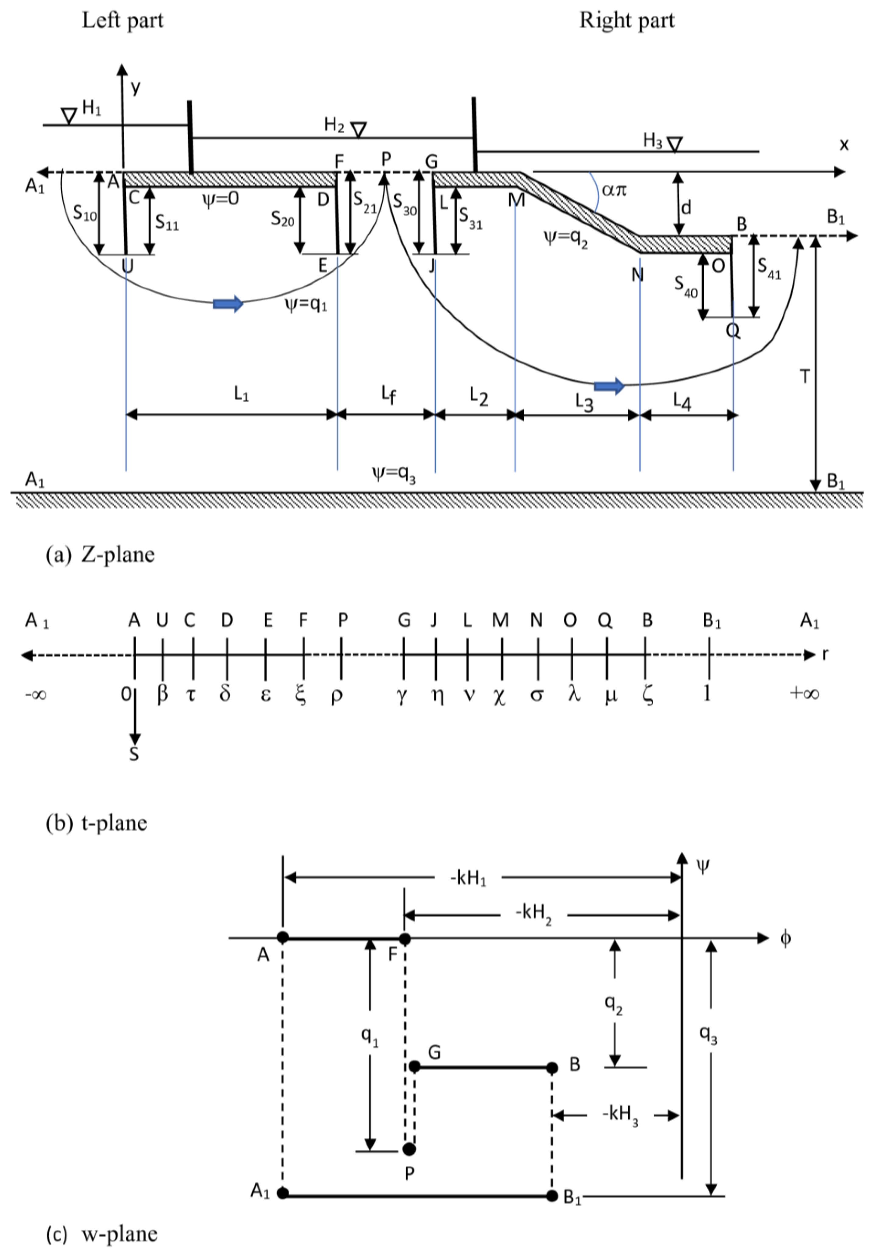
In Figure 1a, the arrangement of two structural elements, along with a filter at an intermediate location and the flow domain in the Z-plane, is depicted. The first structure, referred to as AUCDEF, serves as the upstream barrage and consists of two end sheet piles and a horizontal floor. Within this structure, L₁ represents the distance from point C to point D, S₁₀ indicates the depth at the front face of the sheet pile on the upstream end from point A to point U, and S₁₁ represents the depth at the back face of the sheet pile on the upstream end from point U to C. On the other hand, S₂₀ represents the front face depth of the sheet pile downstream from point D to point E, S₂₁ denotes the back face depth of the downstream sheet pile from point E to F, and L_f signifies the length of the intermediate filter extending from point F to point G.

Figure 1a illustrates the configuration of the downstream structure, known as GJLMNOQB, which consists of a sloping apron in the middle, two sheet piles, and two horizontal aprons. Within this structure, L₂ represents the length of the upstream apron from points L to M, while L₄ signifies the length of the downstream apron from points N to O. The middle apron, spanning from points M to N, is inclined at the “απ” angle with respect to the horizontal axis, and its projected length is denoted as L₃. Additionally, S₃₀ indicates the depth at the front face of the sheet pile on the upstream end from points G to point J, while S₃₁ represents the depth at back face of the sheet pile on the upstream from point J to point L. Similarly, S₄₀ corresponds to the front face depth of the downstream sheet pile from point O to point Q, while S₄₁ signifies the downstream sheet pile depth at the back face from point Q to point B. The parameter d represents the difference in elevation between the upstream and downstream beds. Moreover, H₁ denotes the water level on the upstream side of the existing barrage, H₂ represents the water level within the filter zone, and H₃ signifies the water level on the downstream side of the subsidiary weir. Both structures are constructed upon a finite depth of homogeneous isotropic pervious soil, denoted as T, conforming to the actual field conditions. The complex potential w is mathematically expressed as:

w = ϕ + iψ

where $\psi$ is the stream function; $\varphi$ is the velocity potential function, which is equal to kH, in which H is the total head; and k is the permeability coefficient.

A comprehensive solution to the problem given as $\mathrm{w}=\mathrm{f}\left(\mathrm{z}\right)$ may be derived as given below:

i.

The plane (z), where z = x + iy, is mapped onto the lower half of a supplementary semi-infinite plane t;

ii.

Plane (w) is mapped onto the lower half of the secondary semi-infinite plane t;

iii.

By combining the derived equations, the w–z relationship is obtained.

2.2. Boundary Conditions

According to the illustration in Figure 1a,c, the initial streamline, labeled as ψ = 0, aligns with the boundary at the subsurface of the upstream structural element A, U, C, D, E, F. The upstream segment A₁A, the filter FG at the intermediate location, and the segment BB₁ at the downstream end correspond to lines of equal potential. Without losing the generality, the downstream water level can be chosen as a datum. Then, ${\varphi }_{A1A}=-k{H}_1$, ${\varphi }_{FG}=-k{H}_2$, and ${\varphi }_{BB1}=0.0$, respectively.

Based on the sizes of both structural components, the filter length at the intermediate location, the depth of the stratum, and the ratio of (H₂)/(H₁), three different situations of subsoil flow can occur:

i.

The intermediate filter can be subdivided into two sections, namely from points F to P and from points P to G, where P represents a stagnation point. The first section, extending from point F to point P, serves as an outlet for a portion of the flow from seepage originating from the upstream end. The second section, spanning from points P to G, functions as an inlet face. Consequently, the stream function within this configuration fluctuates in between -q₁ and zero along the FP length, while it transitions in between −q₂ and −q₁ along the PG length (refer to Figure 1a,c). The flow characteristics vary with the variation in length of the intermediate filter. At point F of the intermediate filter, the flow characteristics are defined by the exit gradient. The objective of the safe design of hydraulic structures is to have the exit gradient be in the safe range of values defined by the local codes of practice. At point P of the intermediate structure the flow characteristics are defined by stagnation conditions, while at point G of the intermediate filter the flow is of the infiltration type. It is worth noting further that the net flow is positive and maximum when H₂/H₁ equals zero. This net flow is decreasing as H₂/H₁ is increasing to a certain limit at which the net flow is equal to zero. If H₂/H₁ is increased beyond this point, the net flow will be negative and the entire filter at the intermediate location will work as the inlet face.

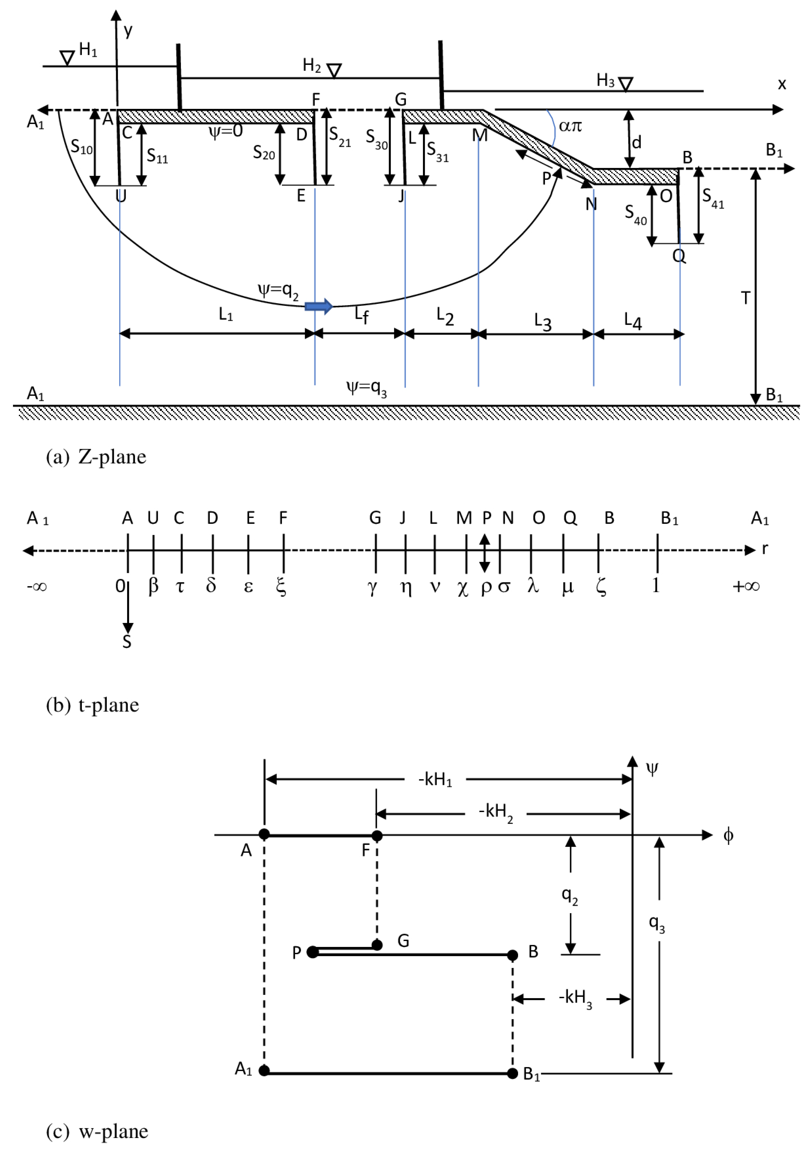
ii.

The streamline, denoted by ψ = −q₂, originates from a point on the upstream bed, which will intersect the downstream structure GJLMNOQB at a certain point P. At this juncture, the streamline splits into two paths: one follows the PG trajectory, culminating at point G, while the other follows the PB trajectory, terminating at the B point. In such special situations, the entire length of the filter at the intermediate location acts as an outlet surface, while the stream function values change along its length, ranging from 0 to −q₂. This information can be observed in Figure 2a,c. At the P point, as given in Figure 2, the head along the downstream structure has its peak value. From that point onwards, the hydraulic head gradually decreases in either direction until it reaches the value equal to H₂ at the G point and eventually decreases to 0 at the B point.

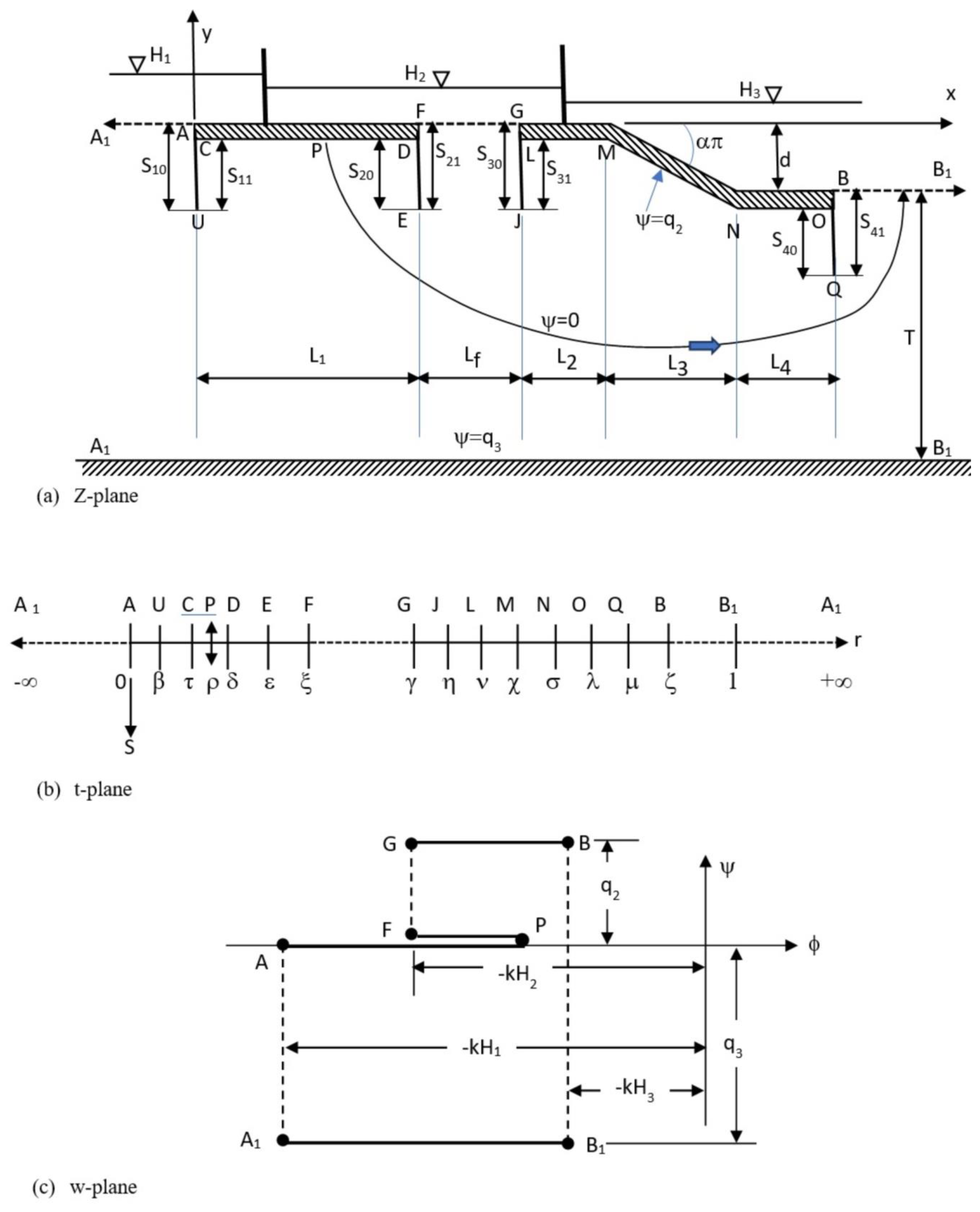
iii.

In this situation, a streamline originating from point A on the upstream bed, having a stream function value of zero, and the other streamline originating from the F point on the filter at the intermediate location, also with a stream function value of zero, intersect at a point P on the upstream structure. From there, they continue their movement towards the bed on the downstream end. The whole of the filter at the intermediate location is to function like an entrance face in this scenario, where the stream function (ψ) values range from 0 to −q₂. Along the upstream floor, the hydraulic head is at its minimum at point P, as illustrated in Figure 3a,c. Moving away from point P, the value of the head rises in either direction until it attains the value of H₂ on the F point and a value equal to H1 on the A point, respectively. Additionally, the streamline corresponding to a stream function value of q₂ aligns with the contour of the subsurface of the structure downstream.

2.3. Analytical Solution

As mentioned earlier, Figure 1a provides a representation of the structure’s geometry, along with the values corresponding to the velocity potential (φ) and the ψ on the boundaries in plane z. The relationship between the quantities φ and ψ is illustrated in Figure 1c, Figure 2c and Figure 3c in the w plane. To conveniently represent points in both plane z and plane w, complex variables are utilized, where z is equal to “x + iy” and w is equal to “φ + iψ”. To solve the given equations, the points in the z plane and w plane are mapped onto points that are common in the secondary plane t. This mapping is demonstrated in Figure 1b, Figure 2b and Figure 3b, employing the transformation described by Schwarz and Christoffel. By using this transformation, the relationships $z=f_1\left(t\right)$. and $w=f_2\left(t\right)$ are established. These relationships allow for the determination of the values of w for all corresponding values of z in principle.

2.3.1. First Operation: $\mathrm{z}={\mathrm{f}}_1\left(\mathrm{t}\right)$

The first operation, denoted as z = f₁(t), involves mapping the polygon A₁AUCDEFGJLMNOQBB₁ in the z plane onto the t plane using the Schwarz–Christoffel equation. This equation is represented as:

$$Z=M_1\underset{0}{\overset{t}{{\displaystyle \int }}}\frac{\left(t-\beta \right)\left(t-\epsilon \right)\left(t-\mathsf{\eta }\right){\left(t-\sigma \right)}^{\alpha }\left(t-\mu \right)dt}{{\left(t-\chi \right)}^{\alpha }\left(t-1\right)\sqrt{t\left(t-\tau \right)\left(t-\delta \right)\left(t-\xi \right)\left(t-\gamma \right)\left(t-\nu \right)\left(t-\lambda \right)\left(t-\zeta \right)}}+N_1$$

(1)

Here, the points A and B₁ (Figure 1a,b) are located at 0 and 1, respectively, while A₁- U- C -D –E- F- G- J- L- M- N -O -Q -B, as shown in Figure 1a,b, are positioned respectively at ∞-β-τ-δ-ε-ξ–γ-η-ν-χ-σ–λ-μ-ζ (unknown variables).

We need to determine the values of these parameters. The inclination angle of the sloping floor MN is denoted by απ, and M₁ and N₁ are complex constants. At the A point, where z is equal to zero and t is equal to zero, N₁ is found to be zero. The value of M₁ is determined by integrating Equation (1) between the limits χ and σ, resulting in:

$$M_1=M_{1r}{e}^{-\mathsf{\alpha }\mathsf{\pi }}$$

where $M_{1r}$ represents the magnitude of $M_1$.

By integrating Equation (1) along the boundaries and dividing this by the length of the floor of the structural element L₁ upstream, the following equations are obtained:

$$R_1=\frac{\left|{{\displaystyle \int }}_0^{\beta }Idt\right|}{\left|{{\displaystyle \int }}_{\tau }^{\delta }Idt\right|}-\frac{S_{10}}{L_1}=0.0$$

(2)

$$R_2=\frac{\left|{{\displaystyle \int }}_{\beta }^{\tau }Idt\right|}{\left|{{\displaystyle \int }}_{\tau }^{\delta }Idt\right|}-\frac{S_{11}}{L_1}=0.0$$

(3)

$$R_3=\frac{\left|{{\displaystyle \int }}_{\tau }^{\epsilon }Idt\right|}{\left|{{\displaystyle \int }}_{\tau }^{\delta }Idt\right|}-\frac{S_{20}}{L_1}=0.0$$

(4)

$$R_4=\frac{\left|{{\displaystyle \int }}_{\epsilon }^{\mathsf{\xi }}Idt\right|}{\left|{{\displaystyle \int }}_{\tau }^{\delta }Idt\right|}-\frac{S_{21}}{L_1}=0.0$$

(5)

$$R_5=\frac{\left|{{\displaystyle \int }}_{\mathsf{\xi }}^{\gamma }Idt\right|}{\left|{{\displaystyle \int }}_{\tau }^{\delta }Idt\right|}-\frac{L_f}{L_1}=0.0$$

(6)

$$R_6=\frac{\left|{{\displaystyle \int }}_{\gamma }^{\mathsf{\eta }}Idt\right|}{\left|{{\displaystyle \int }}_{\tau }^{\delta }Idt\right|}-\frac{S_{30}}{L_1}=0.0$$

(7)

$$R_7=\frac{\left|{{\displaystyle \int }}_{\mathsf{\eta }}^{\nu }Idt\right|}{\left|{{\displaystyle \int }}_{\tau }^{\delta }Idt\right|}-\frac{S_{31}}{L_1}=0.0$$

(8)

$$R_8=\frac{\left|{{\displaystyle \int }}_{\nu }^{\chi }Idt\right|}{\left|{{\displaystyle \int }}_{\tau }^{\delta }Idt\right|}-\frac{L_2}{L_1}=0.0$$

(9)

$$R_9=\frac{\left|{{\displaystyle \int }}_{\chi }^{\sigma }Idt\right|}{\left|{{\displaystyle \int }}_{\tau }^{\delta }Idt\right|}-\frac{L_3}{\cos \left(\alpha \pi \right)L_1}=0.0$$

(10)

$$R_{10}=\frac{\left|{{\displaystyle \int }}_{\sigma }^{\lambda }Idt\right|}{\left|{{\displaystyle \int }}_{\tau }^{\delta }Idt\right|}-\frac{L_4}{L_1}=0.0$$

(11)

$$R_{11}=\frac{\left|{{\displaystyle \int }}_{\lambda }^{\mu }Idt\right|}{\left|{{\displaystyle \int }}_{\tau }^{\delta }Idt\right|}-\frac{S_{40}}{L_1}=0.0$$

(12)

$$R_{12}=\frac{\left|{{\displaystyle \int }}_{\mathsf{\mu }}^{\mathsf{\zeta }}Idt\right|}{\left|{{\displaystyle \int }}_{\tau }^{\delta }Idt\right|}-\frac{S_{41}}{L_1}=0.0$$

(13)

Here, I represents the integrand of Equation (1).

At point B₁ (t = l), as t revolves around a semi-circle of a small radius ($r=\left(t-1\right)e^{-i\theta }$), resulting in a change in z denoted as (iT), we can substitute $t=1+r{e}^{-i\theta }$ and $dt=r{e}^{-i\theta }id\theta$ into Equation (1). This substitution leads to the following equation:

$$T=M_1 \frac{\left(1-\beta \right)\left(1-\epsilon \right)\left(1-\mathsf{\eta }\right){\left(1-\sigma \right)}^{\alpha }\left(1-\mu \right)\pi }{{\left(1-\chi \right)}^{\alpha }\sqrt{\left(1-\tau \right)\left(1-\delta \right)\left(1-\xi \right)\left(1-\gamma \right)\left(1-\nu \right)\left(1-\lambda \right)\left(1-\zeta \right)}}$$

(14)

The residual for Equation (14) can be given as follows (by dividing it by the floor length (L₁), as was done previously for Equations (2)–(13)):

$$R_{13}=\left|\frac{\left(1-\beta \right)\left(1-\epsilon \right)\left(1-\mathsf{\eta }\right){\left(1-\sigma \right)}^{\alpha }\left(1-\mu \right)\pi /\left|{{\displaystyle \int }}_{\tau }^{\delta }I.dt\right|}{{\left(1-\chi \right)}^{\alpha }\sqrt{\left(1-\tau \right)\left(1-\delta \right)\left(1-\xi \right)\left(1-\gamma \right)\left(1-\nu \right)\left(1-\lambda \right)\left(1-\zeta \right)}}\right|-\frac{T}{L_1}$$

(15)

These equations (Equations (2)–(13) and (15)) allow the determination of all the unknown variable because the number of equations matches the number of unknowns.

Since these equations are not explicitly expressed in terms of the transformation parameters, it is not possible to find a direct solution for these parameters. However, these can be solved simultaneously using an iterative method to determine the unknown variables by minimizing the sum of the absolute residuals E:

$$E={{\displaystyle \sum }}_{i=1}^{i=13}{R}_i$$

(16)

Once the values of β, τ, δ, ε, ξ, γ, η, ν, χ, σ, λ, μ, and ζ are known, the variable $M_{1r}$ can be evaluated using the following equation:

$$L_1=M_{1r}\left|{{\displaystyle \int }}_{\tau }^{\delta }Idt\right|$$

(17)

The numerical integration process involved assuming parameters within the range of zero to 1. These parameters were then utilized to estimate the integration using Equations (1)–(13). Subsequently, the error sum, as described in Equation (16), was estimated. The iterative process was repeated until the minimum sum was achieved based on Equation (16). Due to the presence of stagnation points, the conventional numerical integration method was deemed unsuitable. As a result, the Chebyshev technique [25] was employed instead. The integration was carried out using the Chebyshev technique, while the random search method was utilized to assume different parameter values. A FORTRAN code was developed to perform the aforementioned tasks.

2.3.2. Second Operation: ${\mathrm{w} \mathrm{Equal} \mathrm{to} \mathrm{f}}_2\left(\mathrm{t}\right)$

The second operation involves the transformation of the w plane, as shown in Figure 1c, onto the t plane, depicted in Figure 1b. This conformal transformation is represented by the following equation:

$$\frac{dw}{dt}=M_2 \frac{\left(t-\rho \right)}{\sqrt{t\left(t-\xi \right)\left(t-\gamma \right)\left(t-\zeta \right)\left(t-1\right)}}$$

(18)

Here, $M_2$ is a complex constant and ρ is a state variable. Different points on plane w corresponding to plane t are illustrated in Figure 1b,c.

The integration of Equation (18) occurs along the contour at the upstream subsurface, A-U-C-D-E-F, from zero to t, and the following equation is obtained:

$$\varphi +k{H}_1=M_2{{\displaystyle \int }}_0^t\frac{\left(t-\rho \right) dt}{\sqrt{t\left(t-\xi \right)\left(t-\gamma \right)\left(t-\zeta \right)\left(t-1\right)}}$$

(19)

In Equation (19), $\varphi =-kH$ at point F, $\varphi =-k{H}_2$, and $t=\xi$. Thus, we have:

$$k{H}_1-k{H}_2=M_2{{\displaystyle \int }}_0^{\xi }\frac{\left(t-\rho \right) dt}{\sqrt{t\left(t-\xi \right)\left(t-\gamma \right)\left(t-\zeta \right)\left(t-1\right)}}$$

(20)

Similarly, by integrating Equation (18) over the G-J-L-M-N-O-Q-B part from “γ to t”, the following equation is found:

$$\varphi +k{H}_2=M_2{{\displaystyle \int }}_{\gamma }^t\frac{\left(t-\rho \right) dt}{\sqrt{t\left(t-\xi \right)\left(t-\gamma \right)\left(t-\zeta \right)\left(t-1\right)}}$$

(21)

At point B, $\varphi =-k{H}_3=0$ and $t=\zeta$. Therefore, we have:

$$k{H}_2=M_2{{\displaystyle \int }}_{\gamma }^{\zeta }\frac{\left(t-\rho \right) dt}{\sqrt{t\left(t-\xi \right)\left(t-\gamma \right)\left(t-\zeta \right)\left(t-1\right)}}$$

(22)

The constants $M_2$ and $\rho$. can be determined from (20) and (22), considering known values of $\xi ,\gamma , \mathrm{and} \zeta$.

2.4. Potential

In both the first and second operations, the values of $M_{1r}$, β, τ, δ, ε, ξ, γ, η, ν, χ, σ, λ, μ, ζ, $M_2$, and $\rho$. are determined. To calculate the potential at any point along the upstream structure (AUCDEF), one can substitute the corresponding value of t into Equation (19). Similarly, for any point along the downstream structure (GJLMNOQB), the potential can be determined by replacing the equivalent t value into Equation (21). Equation (1) can be utilized to determine the corresponding place of the point under consideration on plane z.

2.5. Exit Gradient

The exit gradient is an important parameter that describes the hydraulic gradient along the downstream bed or intermediate filter. According to [23], the exit gradient, denoted as $I_{exit}$, is calculated at any point using the following equation:

$$I_{exit}=\frac{i}{k}·\frac{dw}{dt}·\frac{dt}{dz}$$

(23)

By employing Equations (1), (18), and (23), the exit gradient can be derived as:

$$I_{exit}=\frac{i}{k}·\frac{M_2}{M_1} \frac{\left(t-\rho \right){\left(t-\chi \right)}^{\alpha }\sqrt{\left(t-1\right)\left(t-\tau \right)\left(t-\delta \right)\left(t-\nu \right)\left(t-\lambda \right)}}{\left(t-\beta \right)\left(t-\epsilon \right)\left(t-\mathsf{\eta }\right){\left(t-\sigma \right)}^{\alpha }\left(t-\mu \right)}$$

(24)

To determine the maximum values of the exit gradient, which may occur at points F, G, and B (as shown in Figure 1a), one can substitute t = ξ, γ, and ζ, respectively, into Equation (24).

2.6. Seepage Flow

Case 1: $\xi <t<\gamma , \mathrm{and} \zeta$

The flow from seepage (q₁), infiltrating into the filter at the intermediate location through the portion FP, and the drained flow (q₂) from the intermediate filter through the portion PG can be determined using the following equations:

$$-i{q}_1=M_2{{\displaystyle \int }}_{\xi }^{\rho }\frac{\left(t-\rho \right) dt}{\sqrt{t\left(t-\xi \right)\left(t-\gamma \right)\left(t-\zeta \right)\left(t-1\right)}}$$

(25)

$$-i{q}_2=M_2{{\displaystyle \int }}_{\xi }^{\gamma }\frac{\left(t-\rho \right) dt}{\sqrt{t\left(t-\xi \right)\left(t-\gamma \right)\left(t-\zeta \right)\left(t-1\right)}}$$

(26)

The seepage flow (q₃), which represents the total flow infiltrating into the downstream bed through the portion BB₁, can be obtained using the following equation:

$$-i{q}_3=M_2{{\displaystyle \int }}_{\zeta }^1\frac{\left(t-\rho \right) dt}{\sqrt{t\left(t-\xi \right)\left(t-\gamma \right)\left(t-\zeta \right)\left(t-1\right)}}+i{q}_2$$

(27)

Case 2: $\xi <\gamma <\rho$

The infiltration flow (q₂) through the filter at the intermediate location can be determined using the equation given below:

$$-i{q}_2=M_2{{\displaystyle \int }}_{\xi }^{\gamma }\frac{\left(t-\rho \right) dt}{\sqrt{t\left(t-\xi \right)\left(t-\gamma \right)\left(t-\zeta \right)\left(t-1\right)}}$$

(28)

The q₃, representing the total flow infiltrating into the downstream bed through the portion BB₁, can be determined with the help of the following equation:

$$-i{q}_3=M_2{{\displaystyle \int }}_{\zeta }^1\frac{\left(t-\rho \right) dt}{\sqrt{t\left(t-\xi \right)\left(t-\gamma \right)\left(t-\zeta \right)\left(t-1\right)}}+i{q}_2$$

(29)

Case 3: $\rho <\xi <\gamma$

The drained infiltration flow (q₂) from the filter at the intermediate location can be calculated using the following equation:

$$-i{q}_2=M_2{{\displaystyle \int }}_{\xi }^{\gamma }\frac{\left(t-\rho \right) dt}{\sqrt{t\left(t-\xi \right)\left(t-\gamma \right)\left(t-\zeta \right)\left(t-1\right)}}$$

(30)

The seepage flow (q₃) infiltrating into the downstream bed through portion BB₁, minus the flow that seeps through the intermediate filter via portion FG, can be obtained from the following equation:

$$-i{q}_3=M_2{{\displaystyle \int }}_{\zeta }^1\frac{\left(t-\rho \right) dt}{\sqrt{t\left(t-\xi \right)\left(t-\gamma \right)\left(t-\zeta \right)\left(t-1\right)}}-i{q}_2$$

(31)

The above-mentioned equations were utilized to calculate the pressures in the upward direction exerted on the downstream and upstream structures, the discharge from seepage, and the gradients at the exit point along the filter at the intermediate location and the bed at the downstream end. To carry out these calculations, numerical methods were employed and multiple integrals were evaluated using a digital computer. For the determination of the variables of Equation (1) corresponding to the actual structural dimensions, the random search method described in [24] was employed, in conjunction with the Gauss–Chebyshev formula [25]. By obtaining the values of $M_2$ and ρ from Equations (20) and (22), respectively, the upward pressure values at critical points associated with the actual structural dimensions were derived using Equations (19) and (21). The obtained results were then used to illustrate the influence of variations in stratum depth (T), structural dimensions, and filter length along with the corresponding active head ration (H₂/H₁) on the features of the seepage flow.

2.7. Finite Element Solution

The finite element technique is employed extensively to analyze subsurface flow in hydraulic structures. Previous studies [26,27] utilized this method to study the seepage underneath the foundation of the Diyala weir in Iraq, with a focus on identifying sheet pile defects resulting from corrosion. Another study [28] employed the finite element method to study the seepage flow under a dam featuring an inclined sheet pile, while [29] used the finite volume method to investigate the seepage under a concrete dam. In another study, ref. [6] used the finite element method to examine the seepage under hydraulic structures equipped with an intermediate filter. Additionally, ref. [30] used the finite element method to determine the optimal angle of inclination for the cutoff underneath the structural elements. Previously, researchers [5] have used slide rule programing to investigate the seepage below hydraulic structures. Other researchers [31] focused on developing a numerical method to investigate the performance of cutoff wall systems in relation to uplift pressure and the piping phenomenon.

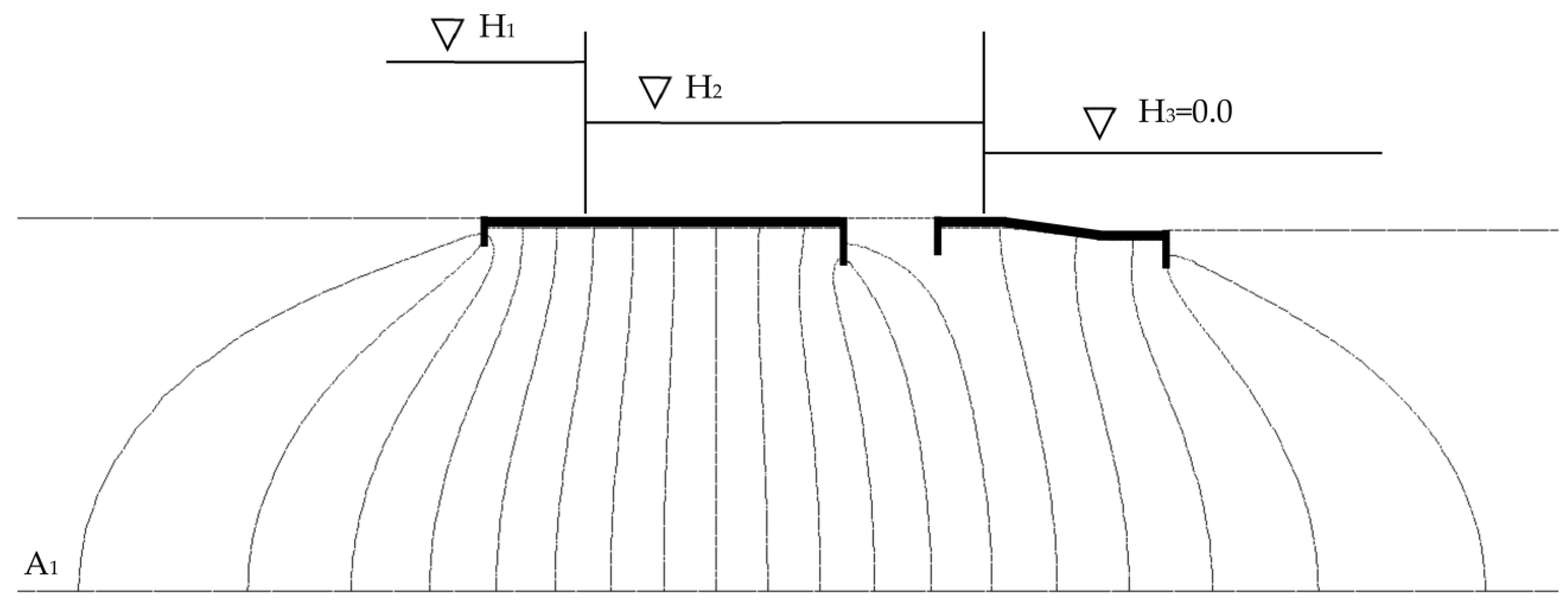
In the present study, we utilized the finite element method to analyze a practical problem involving a barrage with a subsidiary weir, exploring all possible aspects of the problem. The finite element method is extensively described in [32], and for this study we employed the Finite Element Heat Transfer (FEHT) program. The results from FEHT are shown in Figure 4. It is worth mentioning here that the FEHT software has some limitations in drawing all possible graphs. It can be used only to estimate the potential heads, meaning it can draw the equipotential lines only. Additionally, the software can be used to estimate the streamlines but not those corresponding to the equipotential lines. Therefore, the streamlines are not shown in Figure 4. Figure 4 illustrates the equipotential lines for the analyzed sample data, with the following values:

$$\begin{gathered} L1=60 m,\frac{S_{21}}{L_1}=0.125,\frac{L_f}{L_1}=0.25,\frac{S_{10}}{L_1}=0.075,\frac{L_2}{L_1}=0.2,\frac{L_3}{L_1}=0.3,\frac{L_4}{L_1}=0.15, \\ \frac{L_1}{d}=30,\frac{S_{30}}{L_1}=0.1,\frac{S_{41}}{L_1}=0.1,\frac{T}{L_1}=1.0,\frac{t}{L_1}=0.025,\frac{H_2}{H_1}=0.25 \end{gathered}$$

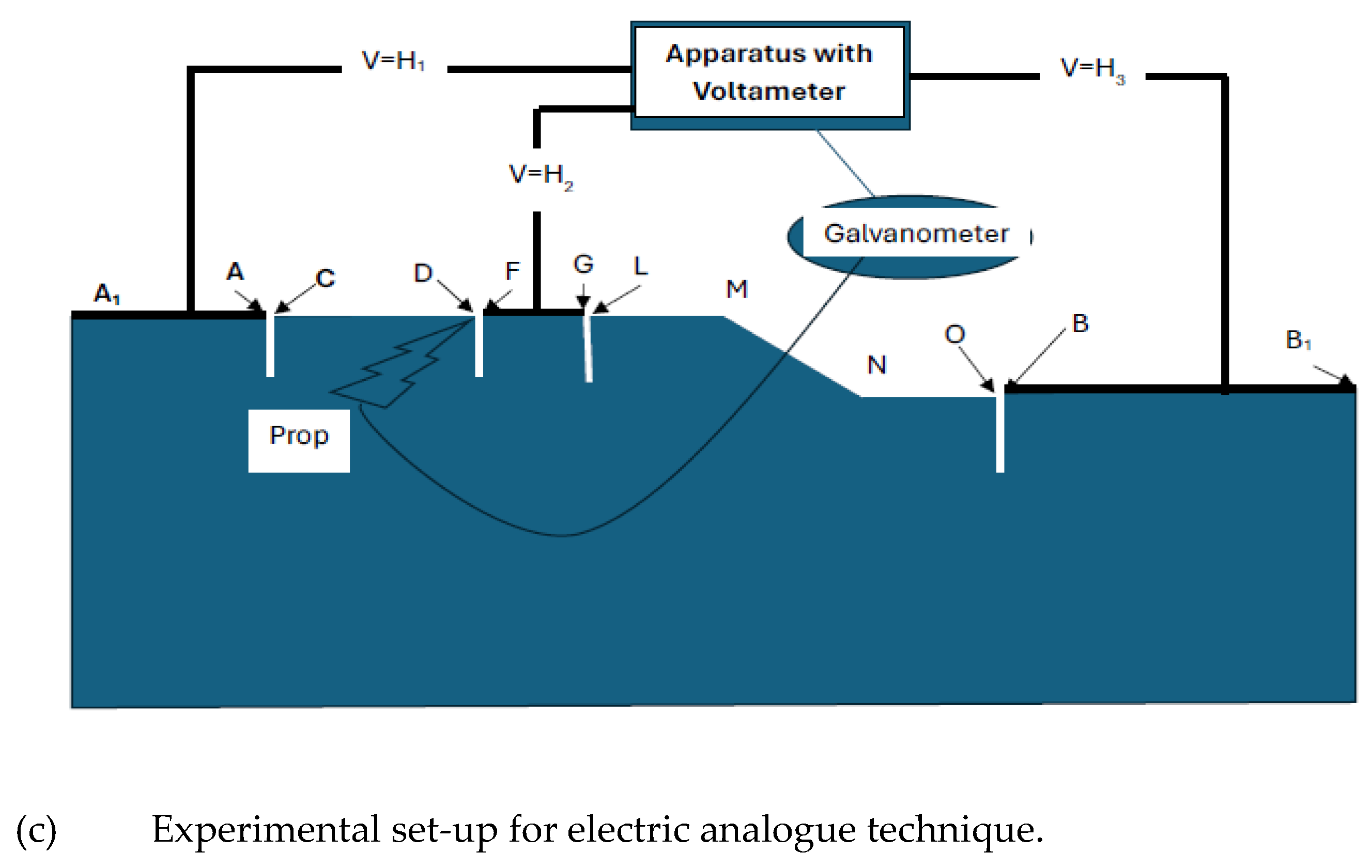
2.8. Experimental Verification

Various methods could be used for the verification of the results obtained from conformal mapping and finite element techniques. A frequency response analysis [33] could be one of the options, physical modeling could be the second one, and analogue experimental techniques could be the third one. The first one requires a large set of data and the second one is very expensive. Therefore, the experimental verification based on the analogue technique was conducted to validate the solution obtained through the implementation of conformal mapping and finite element techniques for the problem at hand. For this purpose, an electric analogue modeling system was prepared, as described by Vaidyanathan [34]. A total of twelve experiments were carried out, utilizing the sample data provided in the previous section, in addition to varying values of the parameter “S₂₁/L₁” (0.10, 0.125, 0.15), along with H₂/H₁ (0.1, 0.25, 0.5, 0.75).

During the experiments, the exerted uplift pressure beneath both the upstream and downstream structures was measured for each combination of S₂₁/L₁ and H₂/H₁ values. These measurements were then compared with the results obtained using the conformal mapping and finite element methods.

3. Results

3.1. Validation of the Models

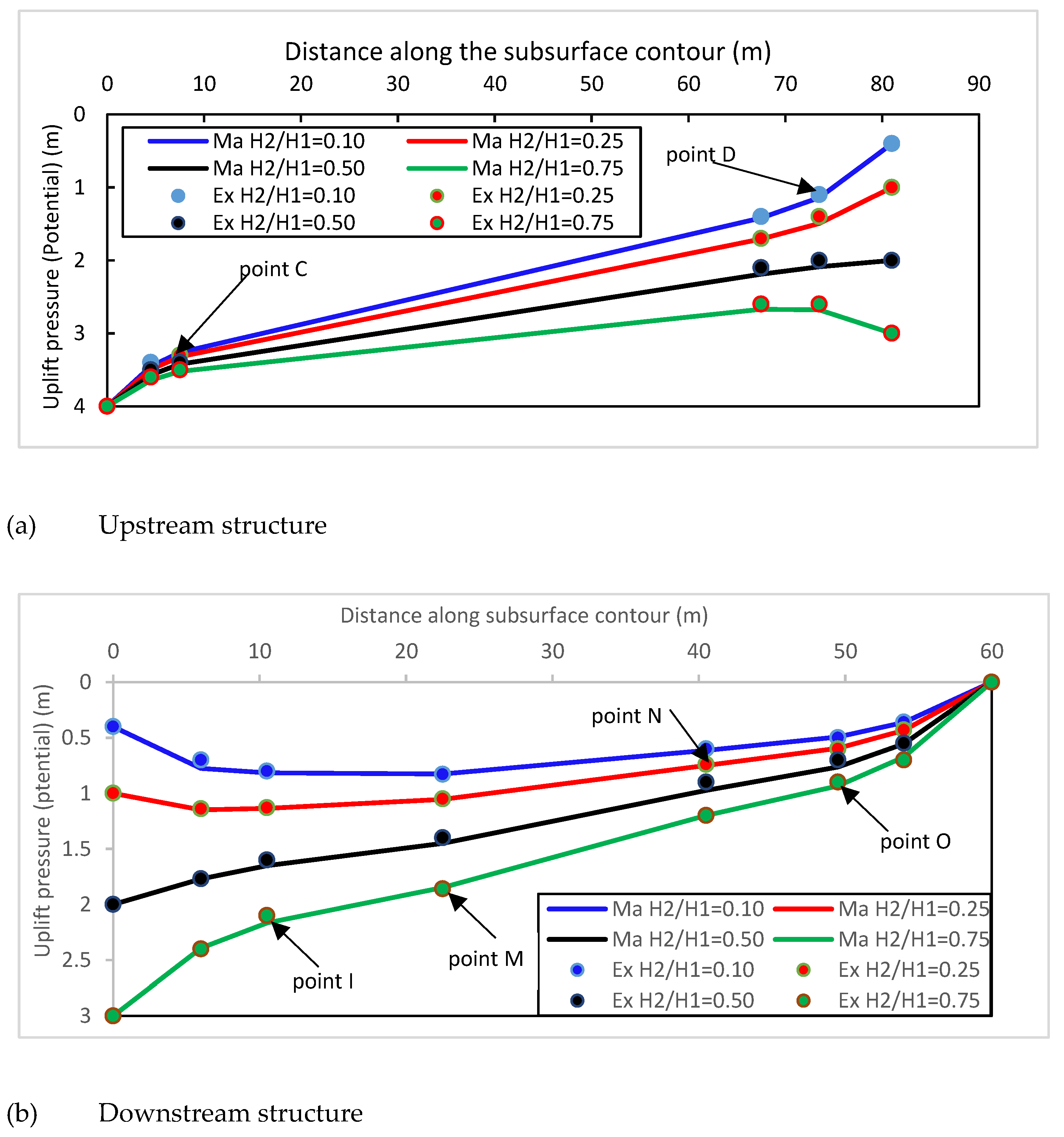
The proposed analytical model was verified for its applicability and accuracy by comparing it with both the electrical analogue method and the numerical method. The comparison of the analytical solution, finite element method, and electric analogue method was conducted for the twelve experiments mentioned earlier, and the results are presented in Figure 5a,b. The experimental setup is given in Figure 5c.

The agreement between the results obtained from the analytical analysis and using the finite element method was found to be excellent, with the maximum percentage deviation between the two results being less than 1%. This indicates a high level of agreement and confirms the accuracy of the analytical method.

Furthermore, the agreement between the data obtained from the analytical solution and the electric analogue experiment was found to be good, with the maximum percentage deviation between the two results being less than 5%. Although slightly higher than the deviation observed with the finite element method, this level of agreement still demonstrates the effectiveness and reliability of the proposed analytical technique.

Figure 5a,b visually represents a comparison between the analytical solution, finite element method, and electric analogue method for the twelve experiments, further supporting the excellent and good agreement observed between these approaches.

In Figure 5b, by going downstream between 0 and 23 m for H₂/H₁ = 0.1, the uplift pressure is increased, which is scenario number 2. The streamline, denoted by ψ = −q₂, originates from a point on the upstream bed, which will intersect the downstream structure GJLMNOQB at a certain point P. At this juncture, the streamline splits into two paths: one follows the PG trajectory, culminating at point G, while the other follows the PB trajectory, terminating at the B point. In the present scenario, the filter at the intermediate location functions as the face at the outlet, while the stream function along its length varies between 0 and −q₂ (refer to Figure 2a,c). The hydraulic head along the downstream structure reaches its maximum value at point P, as depicted in Figure 2, and subsequently decreases in either direction until it achieves a value equal to H₂ at the G point and zero at the B point, respectively. It is noted that Figure 5 shows only the upstream and downstream structures; the impact of the intermediate filter is not presented here.

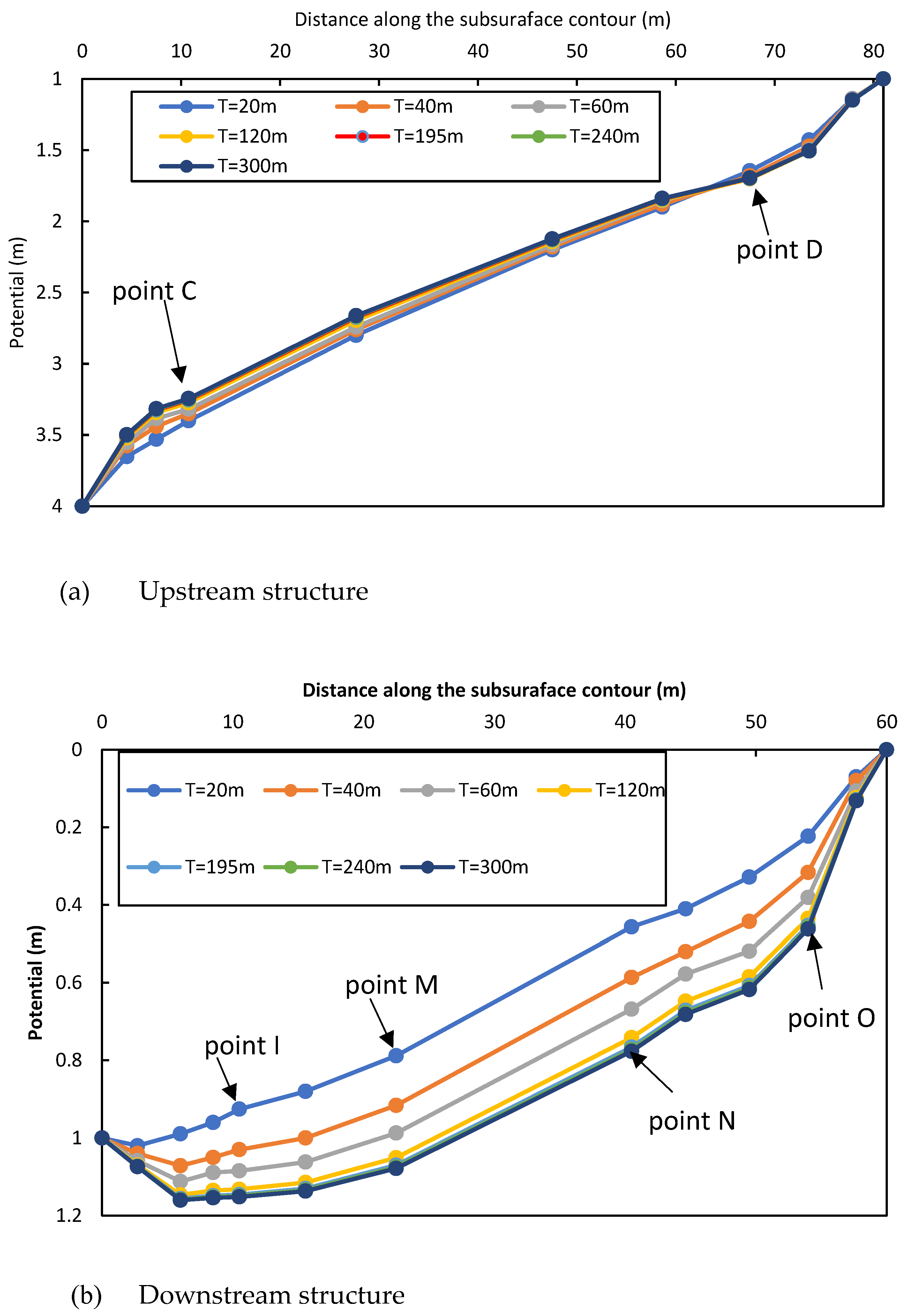
3.2. Effect of the Relative Stratum Depth (T/L₁)

The same dimensions of the upstream and downstream structure as given in the verification section were used with S₂₁/L₁ = 0.125, H₂/H₁ = 0.25, and variable T/L₁ to assess the effect of the relative stratum depth.

The potential acting under the upstream structure was slightly decreased as the relative stratum depth (T/L₁) was increased (Figure 6a). The exit gradient at point F was also slightly decreased as the relative stratum depth (T/L₁) was increased.

Figure 6b shows that the increase in relative stratum depth (T/L₁) results in a larger increase in the upward pressure exerted on the downstream structure compared to that on the upstream structure. There was a 16% increase in potential at some points on the downstream structure due to an increase in stratum depth (T/L₁) from 1.0 to 2.0. The exit gradient at the critical point B was appreciably increased as the relative stratum depth (T/L₁) was increased.

An increase in relative stratum depth (T/L₁) beyond the value of 3 has no effect on the uplift pressure on all points of the upstream and downstream structures. Additionally, the impact of increasing the relative stratum depth (T/L₁) beyond the value of 3 will diminish on the exit gradient at both the F and B points. Therefore, the structures can be dealt with as if founded on an infinite stratum for values of (T/L₁) equal to or greater than 3.

3.3. Effect of the Ratio of the Effective Heads H₂/H₁

For a constant upstream head H1, increasing the ratio of the effective heads H₂/H₁ resulted in a significant increase in potential values along the subsurface contour of the upstream structure (Figure 5a). The gradient at exit point F decreased as the relative head H₂/H₁ increased. The gradient at exit point F continued to decrease until it reached zero, and for further increases in H₂/H₁, point F began to function as an inlet when H₂/H₁ exceeded 0.5.

Figure 5b demonstrates that an increase in the ratio of effective heads led to a noticeable increase in the potential acting on the structure at the downstream end. The gradient at the exit point denoted by B increased as the head ratio H₂/H₁ increased.

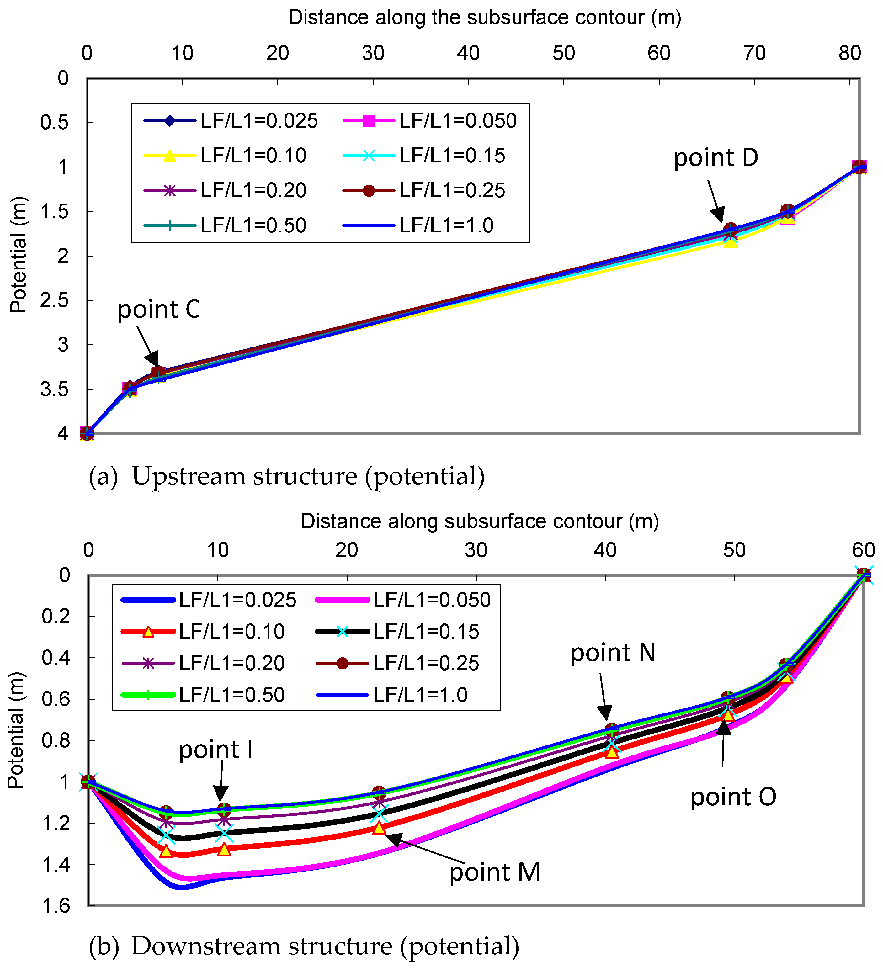
3.4. The Impact of the Relative Length of the Filter (L_f/L₁)

The relative filter length (L_f/L₁) had a slight impact on the potential along the contour at the subsurface of the upstream structure when increased (Figure 7a). However, it significantly decreased the potential along the floor at the downstream end (Figure 7b).

The exit gradient at both points F and B slightly increased with an increase in the filter length until L_f/L₁ reached 0.05. Lengthening the intermediate filter further resulted in a reduction in the gradient at exit points F and B (Figure 7c). However, increasing the filter length beyond a certain point diminished its impact on the exit gradient, and at L_f/L₁ = 3.0, the two structures acted as completely separate structures.

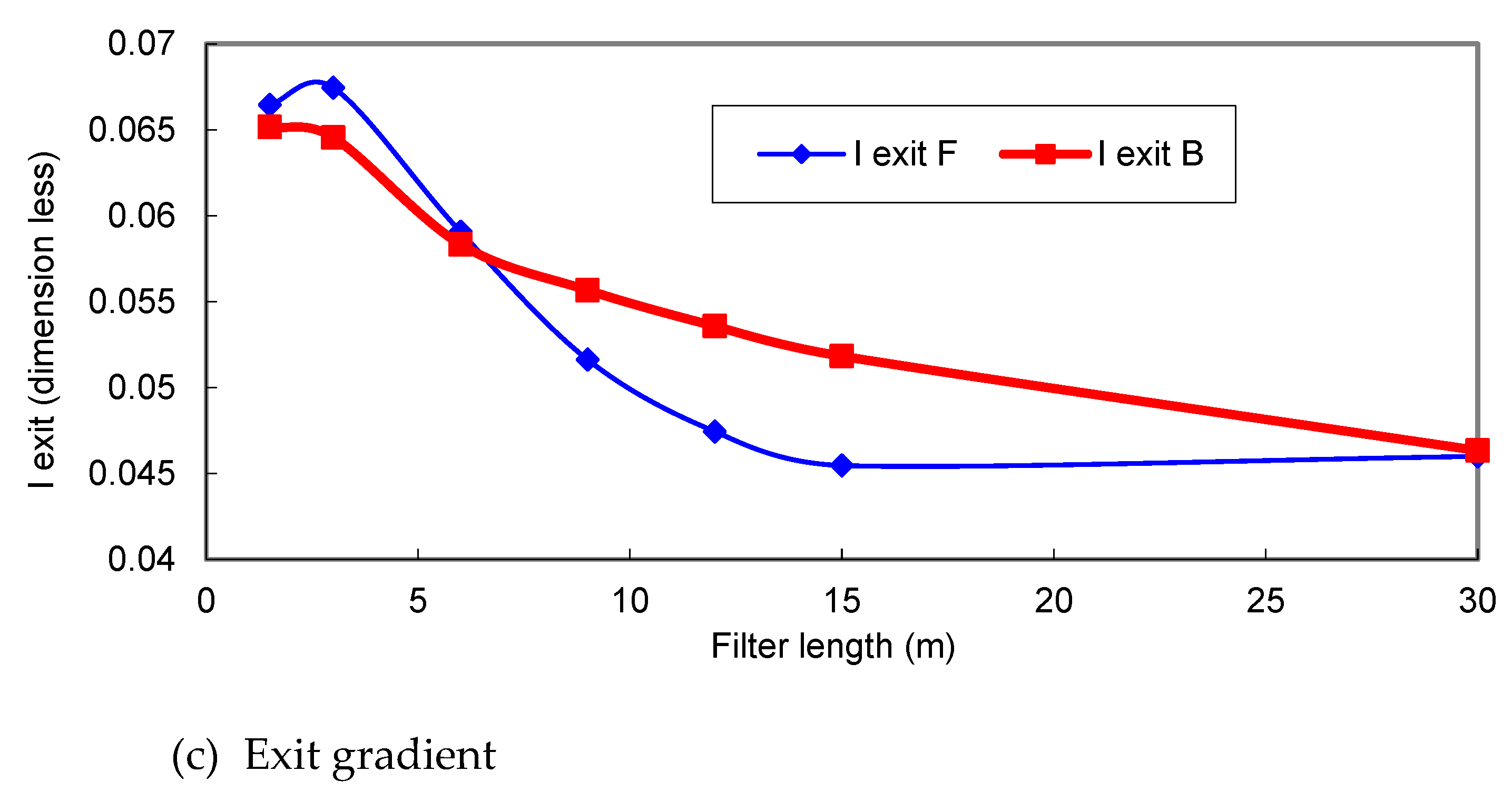
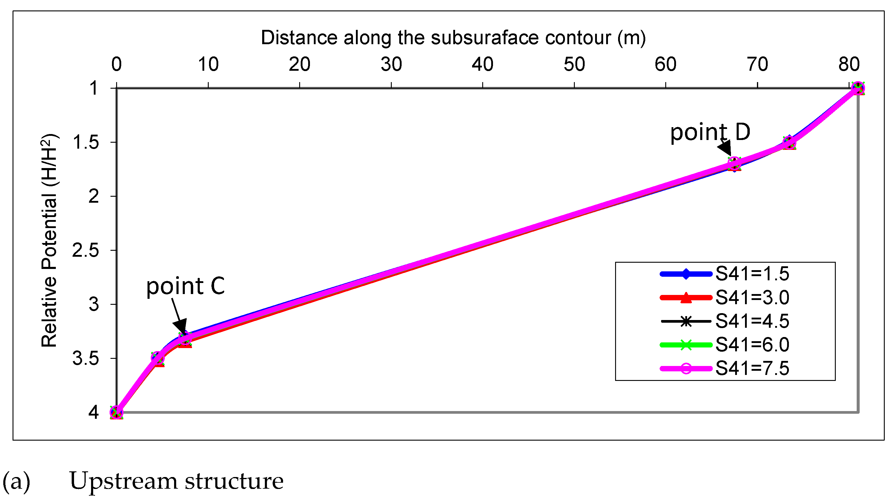
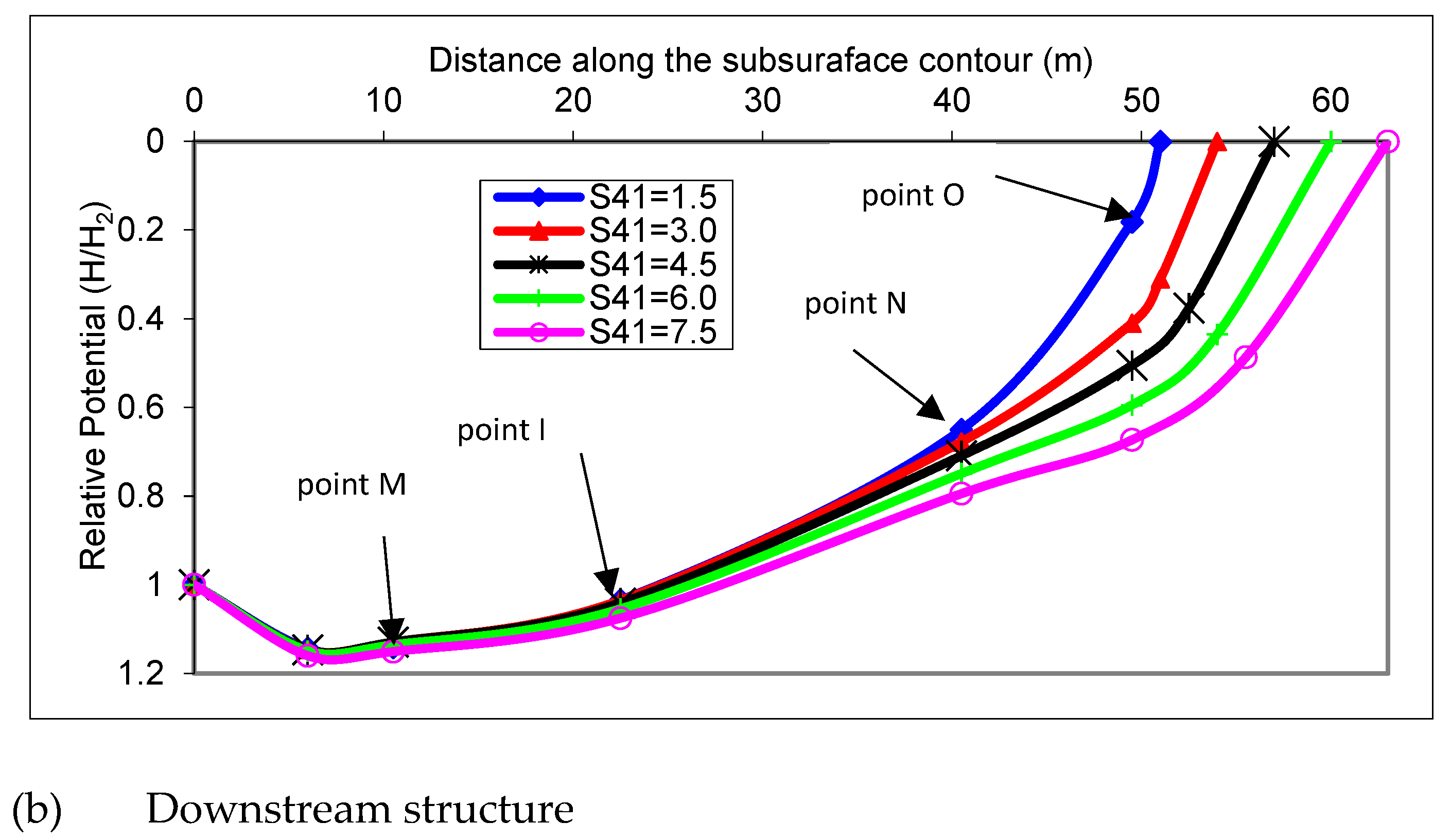
3.5. Effect of the Downstream Sheet Pile at the End of the Downstream Structure (S₄₁)

The downstream sheet pile (S41) at the end of the downstream structure had no effect on the potential along the subsurface contour of the upstream structure, neither did the gradient at the exit point on the downstream area of the upstream structure (Figure 8a,b).

However, it had a significant impact on the potential along the contour in the subsurface strata of the downstream structure and the exit gradient downstream of the structural element. Increasing the sheet pile depth (S₄₁) increased the potential and decreased the exit gradient. The downstream sheet pile depth S₄₁ was recommended to be the minimum essential for ensuring the stability of the subsidiary weir.

4. Summary and Conclusions

The research we conducted focused on addressing the seepage problem beneath a barrage with a subsidiary weir that incorporates an intermediate filter, constructed on finite pervious soil. To find a solution, conformal mapping and finite element methods were employed. The upstream structure, representing an existing barrage, featured a flat floor with two end sheet piles. The proposed subsidiary weir, on the other hand, consisted of upstream and downstream flat aprons, a middle-inclined apron, and two end sheet piles.

Through the use of conformal mapping, a set of equations was derived to simulate various factors. These factors included the potential along the subsidiary weir and existing barrage, the gradients at the exit points along the filter at the intermediate location and the bed at the downstream end, and the seepage flow or the flow draining from the filter at the intermediate location. A computer program was developed to solve these equations.

We also investigated the influence of different parameters on the seepage characteristics. Specifically, the impact of the relative length of the filter (L_f/L₁), the head ratio (H₂/H₁), the relative depth of the stratum (T/L₁), and the presence of downstream sheet piles (S₄₁) were examined.

Based on the conducted research, the following conclusions were made. The behavior of the present barrage and the secondary weir is influenced by the ratio L_f/L₁. When this ratio is less than 3, it affects the behavior of both structures. However, if the ratio exceeds 3, the two structures can be treated as separate entities with independent behavior.

The depth of the stratum also plays a role in the seepage characteristics. If the ratio T/L₁ is less than 3, the behavior of the structures is influenced by the stratum depth. However, if T/L₁ is equal to or greater than 3, the structures can be considered as founded on an infinite stratum, and the impact of the stratum depth becomes negligible.

Regarding the downstream sheet pile S₄₁, it does not affect the seepage characteristics of the upstream structure. Its influence is limited to the seepage characteristics of the downstream structure (subsidiary weir). Therefore, the design considerations for this sheet pile depend solely on ensuring the safety of the downstream structure.

5. Recommendations for Future Research

It is worth mentioning here that in future research, some additional statistical parameters including the root mean square error (RMSE) and Nash–Sutcliffe efficiency (NSE) should be added to the code, along with Equation (16).

References

- Al-Janabi, A.M.S.; Ghazali, A.H.; Yusuf, B.; Sammen, S.S.; Afan, H.A.; Al-Ansari, N.; Shahid, S.; Yaseen, Z.M. Optimizing Height and Spacing of Check Dam Systems for Better Grassed Channel Infiltration Capacity. Appl. Sci. 2020, 10, 3725. [Google Scholar] [CrossRef]
- Yaseen, Z.M.; Ameen, A.M.S.; Aldlemy, M.S.; Ali, M.; Abdulmohsin Afan, H.; Zhu, S.; Sami Al-Janabi, A.M.; Al-Ansari, N.; Tiyasha, T.; Tao, H. State-of-the Art-Powerhouse, Dam Structure, and Turbine Operation and Vibrations. Sustainability 2020, 12, 1676. [Google Scholar] [CrossRef]
- Dawoud, M.A.; El Arabi, N.E.; Khater, A.R.; van Wonderen, J. Impact of rehabilitation of Assiut barrage, Nile River, on groundwater rise in urban areas. J. Afr. Earth Sci. 2006, 45, 395–407. [Google Scholar] [CrossRef]
- Malik, Z.M.; Tariq, A.; Anwer, J. Seepage control for Satpara dam, Pakistan. Proc. Inst. Civ. Eng. Geotech. Eng. 2008, 161, 235–246. [Google Scholar] [CrossRef]
- Alnealy, H.K.T.; Alghazali, N.O.S. Analysis of Seepage Under Hydraulic Structures Using Slide Program. Am. J. Civ. Eng. 2015, 3, 116. [Google Scholar] [CrossRef]
- Ahmed, A.; McLoughlin, S.; Johnston, H. 3D Analysis of Seepage under Hydraulic Structures with Intermediate Filters. J. Hydraul. Eng. 2015, 141, 06014019. [Google Scholar] [CrossRef]
- Sharghi, E.; Nourani, V.; Behfar, N.; Tayfur, G. Data pre-post processing methods in AI-based modeling of seepage through earthen dams. Measurement 2019, 147, 106820. [Google Scholar] [CrossRef]
- Al-Janabi, A.M.S.; Yusuf, B.; Ghazali, A.H. Modeling the Infiltration Capacity of Permeable Stormwater Channels with a Check Dam System. Water Resour. Manag. 2019, 33, 2453–2470. [Google Scholar] [CrossRef]
- Beiranvand, B.; Rajaee, T. Application of artificial intelligence-based single and hybrid models in predicting seepage and pore water pressure of dams: A state-of-the-art review. Adv. Eng. Softw. 2022, 173, 103268. [Google Scholar] [CrossRef]
- Zhu, Y.; Tang, H. Automatic Damage Detection and Diagnosis for Hydraulic Structures Using Drones and Artificial Intelligence Techniques. Remote Sens. 2023, 15, 615. [Google Scholar] [CrossRef]
- Liu, Y.; Zheng, D.; Wu, X.; Chen, X.; Georgakis, C.T.; Qiu, J. Research on Prediction of Dam Seepage and Dual Analysis of Lag-Sensitivity of Influencing Factors Based on MIC Optimizing Random Forest Algorithm. KSCE J. Civ. Eng. 2023, 27, 508–520. [Google Scholar] [CrossRef]
- Al-Janabi, A.M.S.; Ghazali, A.H.; Ghazaw, Y.M.; Afan, H.A.; Al-Ansari, N.; Yaseen, Z.M. Experimental and Numerical Analysis for Earth-Fill Dam Seepage. Sustainability 2020, 12, 2490. [Google Scholar] [CrossRef]
- Singh, R.M. Design of Barrages with Genetic Algorithm Based Embedded Simulation Optimization Approach. Water Resour. Manag. 2010, 25, 409–429. [Google Scholar] [CrossRef]
- Li, P.; He, Z.; Cai, J.; Zhang, J.; Belete, M.; Deng, J.; Wang, S. Identify the Impacts of the Grand Ethiopian Renaissance Dam on Watershed Sediment and Water Yields Dynamics. Sustainability 2022, 14, 7590. [Google Scholar] [CrossRef]
- Kumar, A.; Singh, B.; Chawla, A.S. Design of Structures with Intermediate Filters. J. Hydraul. Eng. 1986, 112, 206–219. [Google Scholar] [CrossRef]
- Salem, A.A.S.; Ghazaw, Y. Stability of two consecutive floors with intermediate filters. J. Hydraul. Res. 2001, 39, 549–555. [Google Scholar] [CrossRef]
- Chawla, A.S. Stability of Structures with Intermediate Filters. J. Hydraul. Div. 1975, 101, 223–241. [Google Scholar] [CrossRef]
- Elganainy, M.A. Flow underneath a pair of structures with intermediate filters on a drained stratum. Appl. Math. Model. 1986, 10, 394–400. [Google Scholar] [CrossRef]
- Elganainy, M.A. Seepage underneath barrages with downstream subsidiary weirs. Appl. Math. Model. 1987, 11, 423–431. [Google Scholar] [CrossRef]
- Farouk, M.I.; Smith, I.M. Design of hydraulic structures with two intermediate filters. Appl. Math. Model. 2000, 24, 779–794. [Google Scholar] [CrossRef]
- Mei, J.; Cao, H.; Luo, G.; Pan, H. Analytical Method for Groundwater Seepage through and Beneath a Fully Penetrating Cut-off Wall Considering Effects of Wall Permeability and Thickness. Water 2022, 14, 3982. [Google Scholar] [CrossRef]
- Mojtahedi, S.H.; Maghrebi, M.F. Closed-form analytical solution for infinite-depth seepage below diversion dams considering the width of cutoff wall. ISH J. Hydraul. Eng. 2023, 1–12. [Google Scholar] [CrossRef]
- Harr, M.E. Groundwater and Seepage; Mc Graw-Hill: New York, NY, USA, 1962. [Google Scholar]
- Swamee, P.K.; Mishra, G.C.; Salem, A.A.S. Optimal Design of Sloping Weir. J. Irrig. Drain. Eng. 1996, 122, 248–255. [Google Scholar] [CrossRef]
- Francis, S. Theory and Problems of Numerical Analysis; Mc Graw-Hill: New York, NY, USA, 1968. [Google Scholar]
- Farmani, S.; Ghaeini-Hessaroeyeh, M.; Hamzehei-Javaran, S. Numerical model of seepage flows by reformulating finite element method based on new spherical Hankel shape functions. Appl. Water Sci. 2023, 13, 8. [Google Scholar] [CrossRef]
- Khassaf, S.I.; Sh, A.; Rasheed, R. Seepage Analysis underneath Diyala Weir Foundation. In Proceedings of the Thirteenth International Water Technology Conference, IWTC 13 2009, Hurghada, Egypt, 12–15 March 2009. [Google Scholar]
- Alsnousi, K.E.; Mohamed, H.G. Effects of Inclined Cutoffs and Soil Foundation Characteristics on Seepage Beneath Hydraulic Structures. In Proceedings of the Twelfth International Water Technology Conference, IWTCl2, Alexandria, Egypt, 1 January 2008; pp. 1597–1617. [Google Scholar]
- Shamsai, A.; Dezfuli, E.A.; Zebardast, A.; Vosoughifar, H.R. A Study of Seepage under a Concrete Dam Using the Finite Volume Method. In Proceedings of the Fourteenth International Water Technology Conference, IWTC14, Cairo, Egypt, 21–23 March 2010; pp. 659–671. [Google Scholar]
- Elmolla, A.M.; Elgalil, W.A.A.; Dardeer, M.A.; Elshimy, A.A. Evaluate the best inclination angle of cutoff beneath hydraulic structures. Int. Res. J. Eng. Technol. 2020, 7, 3966–3974. [Google Scholar]
- Moharrami, A.; Moradi, G.; Bonab, M.H.; Katebi, J.; Moharrami, G. Performance of Cutoff Walls Under Hydraulic Structures Against Uplift Pressure and Piping Phenomenon. Geotech. Geol. Eng. 2015, 33, 95–103. [Google Scholar] [CrossRef]
- Zienkiewicz, O.C.; Taylor, R.L. The Finite Element Method, 5th ed.; McGraw-Hill: Maidenhead, UK, 2000. [Google Scholar]
- Karpenko, M.; Skačkauskas, P.; Prentkovskis, O. Methodology for the Composite Tire Numerical Simulation Based on the Frequency Response Analysis. Eksploatacja i Niezawodność Maint. Reliab. 2023, 25, 1–11. [Google Scholar] [CrossRef]
- Vaidyanathan, V.I. The Application of Electrical Analogy to the Design of Hydraulic Structures; Publication No. 55; Central Board of Irrigation and Power: New Delhi, India, 1955. [Google Scholar]