Highlights
1. What are the main findings?
- CO2–N2 mixture dissolution in brine is examined by considering the cross-diffusion effect for CO2 sequestration in a deep storage reservoir.
- Heterogeneity lowers the average dissolved CO2 and impedes the onset of convection.
2. What is the implication of the main finding?
- Correlations are developed to predict the transition time between the dissolution regimes.
Abstract
The possibility of impure carbon dioxide (CO2) sequestration can reduce the cost of these projects and facilitate their widespread adoption. Despite this, there are a limited number of studies that address impure CO2 sequestration aspects. In this study, we examine the convection–diffusion process of the CO2–nitrogen (N2) mixture dissolution in water-saturated porous media through numerical simulations. Cross-diffusion values, as the missing parameters in previous studies, are considered here to see the impact of N2 impurity on dissolution trapping in more realistic conditions. Homogeneous porous media are used to examine this impact without side effects from the heterogeneity, and then simulations are extended to heterogeneous porous media, which are a good representative of the real fields. Heterogeneity in the permeability field is generated with sequential Gaussian simulation. Using the averaged dissolved CO2 and dissolution fluxes for each case, we could determine the onset of different dissolution regimes and behaviors of dissolution fluxes in CO2–N2 mixture dissolution processes. The results show that there is a notable difference between the pure cases and impure cases. Additionally, a failure to recognize the changes in the diffusion matrix and cross-diffusion effects can result in significant errors in the dissolution process. At lower temperatures, the N2 impurity decreases the amount and flux of CO2 dissolution; however, at higher temperatures, sequestrating the CO2–N2 mixture would be a more reasonable choice due to enhancing the dissolution behavior and lowering the project costs. The results of the heterogeneous cases indicate that heterogeneity, in most cases, reduces the averaged dissolved CO2, and dissolution flux and impedes the onset of convection. We believe that the results of this study set a basis for future studies regarding the CO2–N2 mixture sequestration in saline aquifers.
1. Introduction
The continuous and significant increase in greenhouse gas emissions due to the excessive use of fossil fuels in the industrial production, power, and transportation sectors has caused global warming and climate change [1,2,3]. In order to control greenhouse gas emissions and prevent global warming, carbon dioxide (CO2) capture and storage (CCS) in geological formations is considered a viable tool for reducing atmospheric CO2 concentrations [4,5,6,7,8,9,10,11]. Saline aquifers, depleted oil and gas reservoirs, unmineable coal seams, hydrate storage of CO2 within the subsurface environment, and CO2-based enhanced geothermal systems are the main CO2 storage options in underground geological formations [12,13]. Among these options, saline aquifers have attracted more attention due to their chemistry, permeability, porosity, temperature, pressure, massive capacity for the storage of CO2, wide distribution, and vicinity to the sources of production [6,14,15,16,17,18,19,20]. Involved processes during CCS happen in a fully coupled framework, which is one of the main challenges in this regard. Examining such a complex problem requires a multidisciplinary approach. Here, detailed numerical simulations, which consider these coupled processes, could be helpful, and they supported us in the underlying gaps in our knowledge for a successful CCS project [21,22].
The high cost of CCS in saline aquifers is a barrier to the implementation of these projects, and the possibility of impure CCS (CO2 + impurities) is proposed as a solution to reduce the project cost [23]. Currently, the three main CO2 capture technologies used in large-scale power plants are post-combustion, pre-combustion, and oxyfuel combustion, all of which produce CO2-dominant streams containing impurities [24,25]. It was indicated that impurities have an influence on all types of geological CO2 storage mechanisms [26,27]. Although permitting the existence of impurities in the CO2 streams decreases the cost of CCS projects, it can have undesirable and unknown effects, such as decreased CO2 storage capacity, corrosion, and so on [28].
Nitrogen (N2) is an abundant species in impure CO2 streams [29,30,31]. Accordingly, various studies have been performed to investigate the feasibility of the sequestration of CO2–N2 mixtures in saline aquifers [28,32,33,34,35,36,37,38,39]. From some aspects, N2 injection alongside CO2 is examined, and it seems a suitable solution. For example, N2 is a non-toxic and inert gas that is not present in most aquifers. Previous studies showed that the lower viscosity and water solubility of N2 in comparison to CO2 cause N2 to move in the leading edge of the injected gas, which can be used as a safety signal against leakage in the long-term by monitoring N2 [32,33]. Additionally, during the injection period, N2 increases gas mobility and plume propagation. Hence, the surface area between the injected gas mixture and brine could increase and subsequently enhance the solubility trapping [36,40,41]. The corrosion effects of N2 on the equipment used in the CCS project are negligible. Therefore, there are no safety concerns about damage to equipment with the N2 co-injection [42]. In the CO2–N2-brine system, experimental studies show that N2 increases capillary trapping and causes a reduction in leakage risks through this mechanism [35]. Despite the mentioned advantages, like other impurities, it is believed that N2 reduces the storage capacity of saline aquifers due to the possible reduction of the solubility ratio [43,44] and requires additional investigations on the other aspects.
The estimation of dissolution flux during different dissolution regimes is one of the most significant aspects of the studies mentioned in previous experimental and numerical studies [16,45,46,47,48,49,50,51]. These estimations provide a pragmatic tool for policy and engineering applications to have an initial knowledge about the efficiency of the dissolution process and, consequently, of the storage capacity and project safety in different time scales [52]. During various time scales of CCS, the diffusion coefficient plays an important role. In the injection phase, it controls the viscous fingering and, consequently, the capillary trapping mechanism [8]. Moreover, it is a vital factor for dissolution trapping and, because of that, for mineralization trapping [53,54]. All of these trapping mechanisms are essential to a project’s safety [55]. In previous studies, researchers ignored the impurity effects on the diffusion coefficient due to the complexity of its direct measurement and used the diffusion coefficient of the pure case [28,36,40,41,53,56] to simulate the dissolution process during the impure CCS.
Recently, Omrani et al. [57] provided a data set for the diffusion coefficient of CO2–N2–water systems through the molecular dynamics simulation (shown in Methodology section). These data are validated based on the experimental tests for pure CO2 [57]. However, for the CO2–N2–water systems, there are no experimental data about the cross-diffusion values for validation. However, the data set generally follows up a trend that is observed during our previous experimental tests for the overall effects of the impurity on the diffusion and, consequently, on the onset of convection and dissolution flux [38,39]. Furthermore, we have observed such changes in the diffusion coefficient values, which are measured for specific three-component mixtures (not for impure CO2 in water) [58,59,60].
We considered the effects of heterogeneity in porous media to examine the process in a more realistic condition. Heterogeneity can be examined from structural heterogeneity resulting from fault, fold, or salt diapirs and stratigraphic heterogeneities within facies [61]. Here, we focus on heterogeneous stratigraphic structures within facies. The coupled effect of the gas impurity and heterogeneity in porous media is studied by creating a permeability field through the sequential Gaussian simulation (SGS) [62,63,64].
To the best of the authors’ knowledge, no simulation study has investigated the convective dissolution behavior of complex CO2–N2–water systems by considering the cross-diffusion effects. In this study, we tried to examine the effect of cross-diffusion on convective dissolution behavior in the CO2–N2-water system. We conducted this evaluation based on the amount of dissolved CO2 and the dissolution flux rate through three sets of experiments with mixtures of pure CO2, 90% CO2 + 10% N2, and 80% CO2 + 20% N2. In addition to the homogeneous porous media, which enables us to track the effect of impurity separately, the simulations are followed up on heterogeneous porous media, which are good representatives of the real field conditions. Although great achievements have been made through previous studies on solubility trapping, in this study, we intend to examine the role of N2 impurity in the diffusion–convective dissolution in both homogeneous and heterogeneous porous media. The findings of this study are supposed to provide insights into impure CO2 geological storage and show whether the composition of impurity can be engineered to control the dissolution process, which may be beneficial to the practical deployment of CCS technology.
2. Methodology
To capture the CO2 or CO2 + N2 dissolution in a water-saturated porous medium, a rectangular system away from the injection well was selected as the domain of interest. At distances far enough from the injection well, it can be assumed that the gas-brine contact is horizontal. To examine the behavior of the system through a high-resolution simulation framework, it is essential to use a small-scale domain from the computational costs aspect. A thickness of 10 m is used as the most frequent thickness between the reported aquifers data [60]. The length of the domain is 20 m here. A sharp interface is considered for the gas–water contact, which is a valid assumption for aquifers deeper than 1 km [61,62]. The no-flow boundary conditions are imposed on the side and bottom boundaries of the model. Initial CO2 and N2 concentrations in water are set to zero, and the presence of CO2 or CO2+N2 at the top boundary is represented by the fixed concentrations based on the solubility of CO2 and N2 in brine.
The governing equations in the ternary system are as follows (derived from Kim et al. [54]):
The first equation is the continuity equation, and Equations (2) and (3) are the mass transfer equations for each gas. In these equations, and are porosity and the concentration of dissolved gases, respectively. and are the main diffusion coefficients, and and are the cross-diffusion coefficients. Here, is the velocity vector that can be calculated through Darcy’s law, which describes the motion of Newtonian fluid in the porous medium.
In which , , and are permeability, viscosity, and density, respectively. The mentioned equations are coupled and solved by the finite element method through the COMSOL Multiphysics software to catch the behavior of CO2 or CO2 + N2 dissolution in water. The density of the aqueous phase is calculated by the below equation:
In this equation , , and stand for the molecular weight, density, mole fraction, and partial molar volume, respectively. Furthermore, subscripts , and are used for the resulting solution, water, and dissolved gases. Table 1 lists the model parameters that are used during the simulation. The involved parameters are updated based on pressure and temperature during the simulation. In order to better interpret the convection–diffusion problems, the Rayleigh number is used, which is a dimensionless number and is defined as follows [63]:

Table 1.
The model parameters.
To distinguish the different regimes in the dissolution process, we plotted the dissolution flux versus the logarithm of dimensionless time (). The is defined as where , , and are the time, diffusion coefficient, and height of the system, respectively. Further analyses were performed on these plots to determine the start of the quasi-steady state regime, its dissolution flux, and the starting time of the shut-down regime.
Table 2 lists Fick’s diffusion matrix elements. and are the main diffusion coefficients, and and are the cross-diffusion coefficients. The main diffusion coefficients express the section of the component diffusion that depends on its own concentration gradient, and the cross-diffusion coefficients provide the molar flux of one component driven by the concentration gradient of another component. We applied the molecular dynamic simulation to evaluate the CO2–N2-water diffusion matrix for the first time. For more detail on how these values are calculated, we refer you to our previous work [57].
Table 2.
Fick diffusion coefficients of CO2–N2–water system [57].
In order to investigate the effect of heterogeneity, a random permeability field is created by applying the sequential Gaussian simulation (SGS) algorithm. The SGeMS software was used to generate a normal random distribution in the range of 0−1. The following equation is used to create a log-normal permeability distribution based on the normal random distribution.
where , , , and are the permeability field in the log-normal distribution, the average permeability of the reservoir, the standard deviation of the permeability field, and the permeability field in the standard normal distribution obtained from the SgeMS software, respectively. Each random permeability value generated by this method is assigned to a point in the simulation domain at a specified distance in length, and the permeability between these points is interpolated to reach a continuous field. The average permeability of the reservoir is 250 mD (Table 1), the standard deviation of the permeability field is 1, and the distance length is 1 m in both the and directions. Due to the high difference in distribution pattern from one realization to another, repetition of the simulations for each case is necessary for the results to be reliable. In this regard, considering the computational limitations, we chose 20 realizations for each case.
We conducted a mesh sensitivity analysis to ensure that our results were mesh independent. We selected the most difficult case with the highest Rayleigh number for this purpose. We found that a triangular mesh with a maximum size of 0.1 m is a good choice for this case (and other cases with lower Rayleigh numbers). We considered 4 different triangular meshes: maximum mesh sizes of 0.08, 0.1, and 0.12 m and an adaptive meshing with a maximum size of 0.1 m. Moreso, except for the case with a maximum size of 0.12 m, the average dissolved CO2 for all the other cases overlapped with each other. It should be noted that for the case with a maximum size of 0.1 m, we used 55294 elements to mesh the system, while for the case with a maximum size of 0.08 m, we used 84942 elements. However, we employed an adaptive meshing option in all the simulations to capture the fingers’ movements with a high resolution in some of the high permeability zones of the heterogeneous porous media. We employed adaptive time stepping through the second-order backward differentiation formula (which is a linear multi-step implicit method) to increase the computational speed. To do this, we used 4.375 × 10⁻⁴ years as the first-time step to reach the convergence. Additionally, we used the absolute tolerance of 0.001. The consistent initialization was completed through the backward Euler methodology with 0.001 as the fraction of the initial step. To solve the fully coupled equations, we used the automatic highly nonlinear Newton method with an initial damping factor of 10−4 and a minimum damping factor of 10−8. We restricted the update for step size by a factor of 10. The solver in this numerical model is the Multi-frontal Massively Parallel sparse direct Solver (MUMPS). Here, the recovery damping factor is 0.75. Furthermore, due to the computational restrictions for the gas mixture dissolution process in a 3D heterogeneous porous structure, we used 2D simulations. For the discretization of pressure in Darcy’s law, we used the quadratic approach, and for the concentration values in the mass transfer equation, we employed the linear discretization approach.
3. Results and Discussion
At the beginning of this section, the results of the pure CO2 cases are presented. Then, we discuss the impure cases and the changes that N2 will impose on the dissolution behavior. The simulations are conducted to represent up to 7 years, which is sufficient to catch all the regimes that appear in a dissolution process. For analyzing the CO2 or CO2 + N2 dissolution process, the total concentration of the dissolved gas and dissolution flux, and the dissolution patterns, number, and shape of the convective fingers are considered. Figure 1 shows a schematic of the dissolution behavior. The dissolution process starts with a diffusion-dominated regime. CO2 diffuses into the water due to the concentration gradient. The dissolution flux slows down because of the reduction of the concentration gradient at the interface. The dissolved CO2 + water has a higher density than pure water. This initiates instabilities that lead to the downward motion of dissolved gas and water. As the fingers grow and descend to the bottom, freshwater moves up to the interface to improve the dissolution process. This process continues until the bottom water that moves up to the interface contains dissolved gas. From this stage, the dissolution process moves toward the shut-down regime until a point where the system can no longer dissolve more gas and reaches its maximum capacity. Table 3 lists the details of the pure cases at different temperatures and pressures. Figure 2 illustrates the average dissolved CO2 and dissolution flux for all the pure cases. As was expected, the case with the highest Rayleigh number reaches the higher dissolution flux, and the case with the lowest Rayleigh number ends with the lowest dissolution flux among all the cases. Three cases of 7-p, 8-p, and 9-p almost have the same Rayleigh number; however, the case with a lower diffusion coefficient ends in the higher dissolution flux. This behavior can be seen by comparing the 2-p and 3-p cases. Furthermore, based on the lower solubility of case 3-p, this case would finally result in a lower dissolution capacity. By comparing the dissolution flux curves, it can be interpreted that with the increase of the Rayleigh number, the onset of the quasi-steady and shut-down regimes happens faster, and the dissolution flux of the quasi-steady state regime raises. We fitted and proposed some correlations that relate these parameters to the Rayleigh number. These equations are as follows:
where , , , and are the non-dimensional time of onset of convection, the onset of the quasi-steady state, the onset of the shut-down regime, and the dissolution flux during the quasi-steady regime, respectively.
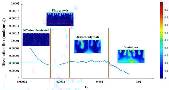
Figure 1.
A schematic of different regimes in a dissolution process.
Table 3.
Details of the pure cases.
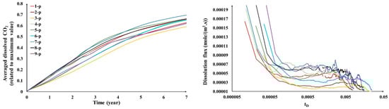
Figure 2.
The averaged dissolved CO2 and dissolution flux for the pure case. Legends for left- and right-hand subplots are same.
For a ternary system of CO2–N2–water, a 2 × 2 matrix of the diffusion coefficient was needed to describe the diffusion behavior. The diagonal elements are the main diffusion coefficients, and the cross-diagonal elements are the cross-diffusion coefficients. In previous studies, for analyzing impure cases, researchers either used the pure diffusion coefficient or the effective diffusion coefficient that was calculated from experimental data, and it was assumed to be independent of concentration for the diluted solution [38,64]. In this study, wherever the diffusion coefficient was needed, we used the summation of the main diffusion coefficient and cross-diffusion coefficient of each component. In other words, for analyzing the CO2 dissolution and for the N2 dissolution behavior (see Equations (2) and (3)) are the effective conditions.
The details on the impure cases of CO2 are listed in Table 4. These data indicate that impure cases do not exactly follow what was expected based on pure cases. The dissolution flux does not act in accordance with the Rayleigh number. In the pure cases, we observed a relation between the increase of the Rayleigh number and the dissolution flux, yet there are contradictions of this relation in the impure cases. In comparison to the pure cases, it seems that at higher pressure, there is no noticeable reduction in the dissolution flux, and it is either the same as the pure cases or has a higher value. However, at lower pressure, the change in dissolution flux can be considerable. Other than the dissolution flux, there are special relations between the Rayleigh number with , , and . The cases with a higher Rayleigh number have a faster onset of convection, quasi-steady and shut-down regimes. We proposed the following correlations for predicting the , and of impure cases:
Table 4.
Details of the impure CO2 cases.
These equations are in good agreement with our previous studies that show impurities in the system of CO2–water (such as different types of gases and salts) and demonstrate a drastic impact on the CO2 dissolution parameters [48]. We conducted all simulations with and without considering cross-diffusion to check the influence of the diffusion coefficient on the dissolution behavior. Figure 3 shows the averaged dissolved CO2 and dissolution flux of all the impure cases. It is obvious that there is a clear difference between these two sets of simulations. It can be implied that ignoring the changes in the diffusion coefficient can cause significant errors in the dissolution process parameters. For example, if we do not consider the change in the diffusion matrix, case 1-i reaches the average dissolved CO2 of about 0.3 (Figure 3c); however, by applying these changes, it reaches the final value of almost 0.4 (Figure 3a). Moreover, by looking at the dissolution flux curves, the noticeable alteration of the onset of different regimes and dissolution flux is indisputable. Referring to the impure cases with consideration given to cross-diffusion (Figure 3, first and third rows), higher or lower Rayleigh numbers do not necessarily lead to higher or lower dissolved CO2 or dissolution flux. Furthermore, these results imply that reducing the CO2 main diffusion coefficient at higher temperatures results in a higher amount of dissolved CO2 and dissolution flux. By comparing cases 13-i and 17-i, we can see that case 17-i, even with a lower Rayleigh number than case 13-i, has the highest amount of dissolved CO2 and dissolution flux among all impure cases, with 90% CO2-10% N2.
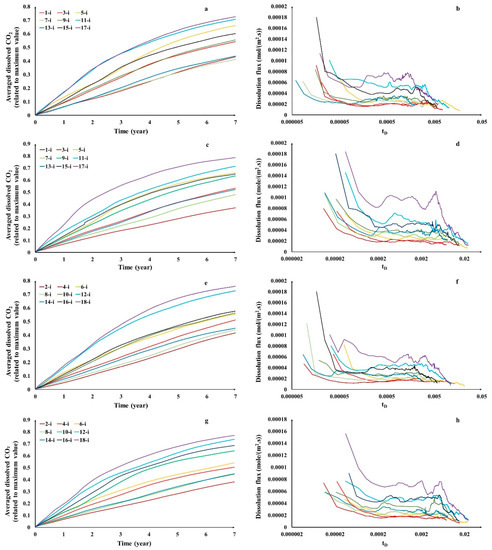
Figure 3.
The averaged dissolved CO2 and dissolution flux for the systems of 90% CO2-10% N2 with considering cross-diffusion (a,b) and without considering cross-diffusion (c,d); the systems of 80% CO2-20% N2 with considering cross-diffusion (e,f) and without considering cross-diffusion (g,h). Legends for left- and right-hand subplots are same.
Suppose we consider cases based on their temperature, as in Figure 4, at 323 K, then the difference between the pure and impure cases is obvious, both in the average dissolved CO2 and dissolution flux. This suggests that in a reservoir with lower temperatures, it is probably better to sequester pure CO2. At a temperature of 373 K, the pure cases show a higher amount of dissolved CO2 and dissolution flux than the impure cases, but the differences are insignificant. Due to the high costs of purifying the injection stream, impure CO2 storage can be a more reasonable choice. At 423 K, the 90% CO2-10% N2 cases reach higher dissolved CO2 and dissolution flux than the pure cases. Therefore, injection of CO2 with N2 in reservoirs with high temperatures can lead to higher dissolved CO2, higher dissolution flux, and a faster onset of quasi-state and shut-down regimes in the dissolution process. Figure 5 illustrates the dissolved CO2 pattern at the times of the onset of convection, flux growth, the onset of a quasi-steady state, and the onset of the shut-down regime for 7-p, 13-i, 9-p, and 18-i. At early times, the activation of the convective flow holds the intense decrease of dissolution flux, and the convective fingers grow independently; however, as time progresses, these fingers grow and interact with each other in different patterns, which are discussed in our previous work [48]. The higher number and faster descending motion of convective fingers bring more freshwater to the interface, which leads to the enhancement of the diffusion–convection mass transfer rate and CO2 dissolution flux. In Figure 5, if we compare cases with higher dissolved CO2 (cases 7-p and 18-i) with lower ones, a special pattern can be identified in the number and interaction of convective fingers. Due to the restriction of lateral movement at the side boundaries, the downward finger motion at these sites may be faster. The comparison of cases 7-p and 13-i confirm the reduction of dissolved CO2 and dissolution flux due to the addition of 10% N2 into the injection stream. Despite this, case 18-i has the highest dissolved CO2 ratio among the impure cases, appears to have more convective fingers, and, therefore, has a stronger convection flow than its pure case (9-p). These patterns, alongside the previous findings, show the effects and importance of N2 impurity on the CO2 dissolution process. Figure 6 shows the averaged dissolved N2 and dissolution flux for the impure cases. It can be seen that, in most cases, there is no convection regime, and there is only a monotonic downward trend. At lower pressures, the N2 diffusion coefficient drastically increases, leading to a stronger diffusion-dominated flow, but at higher pressures, there are indications of a convective flow.
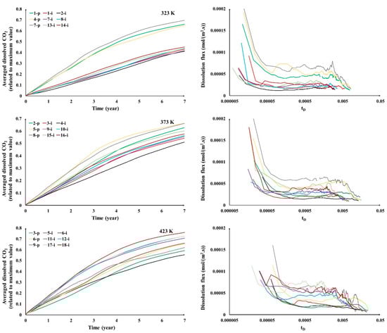
Figure 4.
The averaged dissolved CO2 and dissolution flux for pure and impure cases classified based on temperature. Legends for left- and right-hand subplots are same.
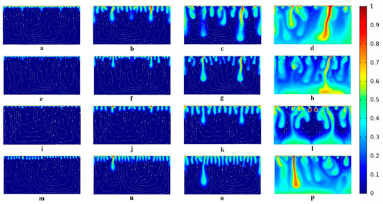
Figure 5.
Dissolved CO2 patterns for cases 7-p (first row), 13-i (second row), 9-p (third row), and 18-i (fourth row): (a) case 7-p at = 0.00017; (b) case 7-p at = 0.00055; (c) case 7-p at = 0.00108; (d) case 7-p at = 0.00301; (e) case 13-i at = 0.00007; (f) case 13-i at = 0.00017; (g) case 13-i at = 0.00034; (h) case 13-i at = 0.00125; (i) case 9-p at = 0.00025; (j) case 9-p at = 0.0007; (k) case 9-p at = 0.00157; (l) case 9-p at = 0.00535; (m) case 18-i at = 0.00011; (n) case 18-i at =0.00036; (o) case 18-i at = 0.00071; (p) case 18-i at = 0.00324.
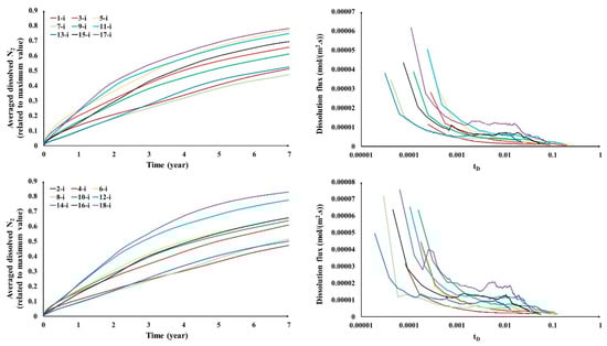
Figure 6.
The averaged dissolved N2 and dissolution flux for impure cases. Legends for left- and right-hand subplots are same.
We developed the dissolution model to include the reservoir heterogeneity in permeability in the presence of the fluid’s cross-diffusion effect. We chose five cases of 1-i, 2-i, 3-i, 4-i, and 9-i (see Table 4). Figure 7, Figure 8, Figure 9, Figure 10 and Figure 11 display these cases. We depicted all the realizations for each case (dotted lines) beside the curves for the homogeneous system with and without considering the cross-diffusion (solid line and dashed line, respectively). Almost in all cases, heterogeneity decreases the averaged amount of dissolved CO2. Furthermore, it can be seen that it impedes the onset of the convective regime and lowers the dissolution flux. Intuitively, heterogeneity increases the uncertainty and complexity of a system. To demonstrate a clearer picture, we averaged the results of all the realizations for each case (Figure 12). Detecting the onset of convection in Figure 12 is indistinct visually. However, it is well known that the onset of convection corresponds to the minimum dissolution flux, and we can estimate this point from Figure 12 or measure it from the dissolution flux data. It should be noted that this behavior comes from the combined effect of heterogeneity in porous media and cross-diffusion from the impurity. By comparing the homogeneous and heterogeneous cases of 3-i and 9-i (Figure 3a and Figure 12), it can be inferred that heterogeneity increases the separation between these two cases and has a stronger impact at lower pressures.
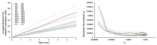
Figure 7.
The heterogeneous realizations (dotted lines), homogeneous with considering cross-diffusion (solid line), and homogeneous without considering cross-diffusion (dashed line) averaged dissolved CO2 and dissolution flux for case 1-i. Legends for left- and right-hand subplots are same.
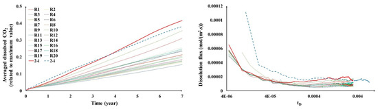
Figure 8.
The heterogeneous realizations (dotted lines), homogeneous with considering cross-diffusion (solid line), and homogeneous without considering cross-diffusion (dashed line) averaged dissolved CO2 and dissolution flux for case 2-i. Legends for left- and right-hand subplots are same.
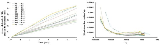
Figure 9.
The heterogeneous realizations (dotted lines), homogeneous with considering cross-diffusion (solid line), and homogeneous without considering cross-diffusion (dashed line) averaged dissolved CO2 and dissolution flux for case 3-i. Legends for left- and right-hand subplots are same.
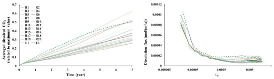
Figure 10.
The heterogeneous realizations (dotted lines), homogeneous with considering cross-diffusion (solid line), and homogeneous without considering cross-diffusion (dashed line) averaged dissolved CO2 and dissolution flux for case 4-i. Legends for left- and right-hand subplots are same.
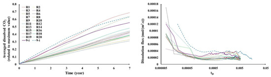
Figure 11.
The heterogeneous realizations (dotted lines), homogeneous with considering cross-diffusion (solid line), and homogeneous without considering cross-diffusion (dashed line) averaged dissolved CO2 and dissolution flux for case 9-i. Legends for left- and right-hand subplots are same.
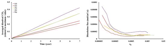
Figure 12.
The averaged dissolved CO2 and dissolution flux averaged for all the realizations of heterogeneous cases. Legends for left- and right-hand subplots are same.
4. Conclusions
In this study, we examined the CO2–N2 mixture dissolution in water-saturated porous media by considering the cross-diffusion effects through numerical simulations. Furthermore, we extended our study by including permeability heterogeneity in our simulations. The analysis of pure CO2 dissolution reveals a relationship between the Rayleigh number and different quantification parameters of the dissolution process, including the dissolution flux and transition time. We proposed some correlations to predict the onset of convection, the onset of a quasi-steady state, the onset of a shut-down regime, and the dissolution flux of pure cases. The key takeaway point is that, despite the pure CO2 in which the dissolution flux could be estimated based on the Rayleigh number, more complexity arises from the cross-diffusion in the CO2–N2–water system. It seems that at lower temperatures, the N2 impurity highly impacts and lowers the CO2 dissolution; however, at higher temperatures, sequestrating the CO2–N2 mixture could be a more reasonable choice, either because of being an economically more feasible option or enhancing the CO2 dissolution behavior. We also proposed some relations based on the Rayleigh number to predict the onset of convection, the onset of the quasi-steady state, and the onset of the shut-down regime for CO2–N2 cases. The interpretation of the heterogeneous cases implies that heterogeneity, in most cases, decreases the averaged dissolved CO2, weakens the convective flow, and lowers the dissolution flux. Moreover, a stronger influence on the dissolution process at lower pressures is possible. The outcomes of this study declare that ignoring the changes in the diffusion matrix and cross-diffusion effects can cause major errors in predicting CO2–N2 mixture dissolution behavior. We hope that the results of this study pave the way for future studies regarding impure CO2 sequestration in saline aquifers.
Author Contributions
Conceptualization, S.M., M.S., R.M., S.O. and I.S.; Methodology, S.M., M.S., R.M. and S.O.; Software, S.M. and M.S.; Validation, S.M., M.S., R.M. and S.O.; Formal analysis, S.M., M.S., R.M. and S.O.; Investigation, S.M., M.S., R.M., S.O. and I.S.; Resources, I.S.; Data curation, S.M., M.S. and R.M.; Writing—original draft, S.M., M.S., R.M. and S.O.; Writing—review & editing, S.M., M.S., R.M. and I.S.; Visualization, S.M., M.S. and R.M.; Supervision, I.S.; Project administration, I.S.; Funding acquisition, I.S.. All authors have read and agreed to the published version of the manuscript.
Funding
The work has received funding from the FiF with project number 40101383. Authors have received support from the Group of Geothermal Science and Technology, Institute of Applied Geosciences, Technische Universität Darmstadt.
Acknowledgments
Authors have received support from the Group of Geothermal Science and Technology, Institute of Applied Geosciences, Technische Universität Darmstadt. We acknowledge support by the Deutsche Forschungsgemeinschaft (DFG, German Research Foundation) and the Open Access Publishing Fund of Technical University of Darmstadt.
Conflicts of Interest
On behalf of all authors, the corresponding authors states that there is no conflict of interest.
References
- Rubin, E.; De Coninck, H. IPCC Special Report on Carbon Dioxide Capture and Storage; Cambridge University Press: Cambridge, UK, 2005; p. 14. [Google Scholar]
- Wang, K.; Xu, T.; Wang, F.; Tian, H. Experimental study of CO2–brine–rock interaction during CO2 sequestration in deep coal seams. Int. J. Coal Geol. 2016, 54, 265–274. [Google Scholar] [CrossRef]
- Ajayi, T.; Awolayo, A.; Gomes, J.; Parra, H.; Hu, J. Large scale modeling and assessment of the feasibility of CO2 storage onshore abu dhabi. Energy 2019, 185, 653–670. [Google Scholar] [CrossRef]
- Bradshaw, J.; Bachu, S.; Bonijoly, D.; Burruss, R.; Holloway, S.; Christensen, N.P.; Mathiassen, O.M. CO2 storage capacity estimation: Issues and development of standards. Int. J. Greenh. Gas Control. 2007, 1, 62–68. [Google Scholar] [CrossRef]
- Talebian, M.; Al-Khoury, R.; Sluys, L. A computational model for coupled multiphysics processes of CO2 sequestration in fractured porous media. Adv. Water Resour. 2013, 59, 238–255. [Google Scholar] [CrossRef]
- Soltanian, M.R.; Amooie, M.A.; Dai, Z.; Cole, D.; Moortgat, J. Critical dynamics of gravito-convective mixing in geological carbon sequestration. Sci. Rep. 2016, 6, 1–13. [Google Scholar] [CrossRef]
- Du, S.; Su, X.; Xu, W. Assessment of CO2 geological storage capacity in the oilfields of the Songliao Basin, North Eastern China. Geosci. J. 2016, 20, 247–257. [Google Scholar] [CrossRef]
- Singh, M.; Chaudhuri, A.; Chu, S.; Stauffer, P.; Pawar, R. Analysis of evolving capillary transition, gravitational fingering, and dissolution trapping of CO2 in deep saline aquifers during continuous injection of supercritical CO2. Int. J. Greenh. Gas Control 2019, 82, 281–297. [Google Scholar] [CrossRef]
- Singh, M.; Chaudhuri, A.; Stauffer, P.; Pawar, R. Simulation of gravitational instability and thermo-solutal convection during the dissolution of CO2 in deep storage reservoirs. Water Resour. Res. 2020, 56, e2019WR026126. [Google Scholar] [CrossRef]
- Amarasinghe, W.; Fjelde, I.; Rydland, J.-A.; Guo, Y. Effects of permeability on CO2 dissolution and convection at reservoir temperature and pressure conditions: A visualization study. Int. J. Greenh. Gas Control 2020, 99, 103082. [Google Scholar] [CrossRef]
- Amarasinghe, W.; Fjelde, I.; Giske, N.; Guo, Y. CO2 convective dissolution in oil-saturated unconsolidated porous media at reservoir conditions. Energies 2021, 14, 233. [Google Scholar] [CrossRef]
- Riaz, A.; Cinar, Y. Carbon dioxide sequestration in saline formations: Part 1—Review of the modeling of solubility trapping. J. Pet. Sci. Eng. 2014, 124, 367–380. [Google Scholar] [CrossRef]
- Emami-Meybodi, H.; Hassanzadeh, H.; Green, C.; Ennis-King, J. Convective dissolution of CO2 in saline aquifers: Progress in modeling and experiments. Int. J. Greenh. Gas Control 2015, 40, 238–266. [Google Scholar] [CrossRef]
- Mahmoodpour, S.; Rostami, B. Design-of-experiment-based proxy models for the estimation of the amount of dissolved CO2 in brine: A tool for screening of candidate aquifers in geo-sequestration. Int. J. Greenh. Gas Control 2017, 56, 261–277. [Google Scholar] [CrossRef]
- Soltanian, M.; Amooie, M.; Cole, D.; Darrah, T.; Graham, D.; Pfiffner, S.; Phelps, T.; Moortgat, J. Impacts of methane on carbon dioxide storage in brine formations. Groundwater 2018, 56, 176–186. [Google Scholar] [CrossRef] [PubMed]
- Jun, Y.-S.; Giammar, D.; Werth, C. Impacts of Geochemical Reactions on Geologic Carbon Sequestration. Environ. Sci. Technol. 2013, 47, 3–8. [Google Scholar] [CrossRef]
- Soltanian, M.R.; Hajirezaie, S.; Hosseini, S.A.; Dashtian, H.; Amooie, M.A.; Meyal, A.; Ershadnia, R.; Ampomah, W.; Islam, A.; Zhang, X. Multicomponent reactive transport of carbon dioxide in fluvial heterogeneous aquifers. J. Nat. Gas Sci. Eng. 2019, 65, 212–223. [Google Scholar] [CrossRef]
- Zhang, W.; Xu, T.; Li, Y. Modeling of fate and transport of coinjection of H2S with CO2 in deep saline formations. J. Geophys. Res. Solid Earth 2011, 116. [Google Scholar] [CrossRef]
- Davison, J.; Thambimuthu, K. An overview of technologies and costs of carbon dioxide capture in power generation. Proc. Inst. Mech. Eng. Part A J. Power Energy 2009, 223, 201–212. [Google Scholar] [CrossRef]
- Jacquemet, N.; Picot-Colbeaux, G.; Vong, C.Q.; Lions, J.; Bouc, O.; Jérémy, R. Intrusion of CO2 and impurities in a freshwater aquifer—Impact evaluation by reactive transport modelling. Energy Procedia 2011, 4, 3202–3209. [Google Scholar] [CrossRef]
- Bachu, S. CO2 storage in geological media: Role, means, status and barriers to deployment. Prog. Energy Combust. Sci. 2008, 34, 254–273. [Google Scholar] [CrossRef]
- Jiang, X. A review of physical modelling and numerical simulation of long-term geological storage of CO2. Appl. Energy 2011, 88, 3557–3566. [Google Scholar] [CrossRef]
- Li, D.; Jiang, X.; Meng, Q.; Xie, Q. Numerical analyses of the effects of nitrogen on the dissolution trapping mechanism of carbon dioxide geological storage. Comput. Fluids 2015, 114, 1–11. [Google Scholar] [CrossRef]
- Wilkinson, M.; Boden, J.; Panesar, R.; Allam, R. CO2 capture via oxyfuel firing: Optimisation of a retrofit design concept for a refinery power station boiler. In Proceedings of the First National Conference on Carbon Sequestration, Washington DC, USA, 15–17 May 2001; Volume 5, pp. 15–17. [Google Scholar]
- Pipitone, G.; Bolland, O. Power generation with CO2 capture: Technology for CO2 purification. Int. J. Greenh. Gas Control 2009, 3, 528–534. [Google Scholar] [CrossRef]
- Porter, R.T.; Fairweather, M.; Pourkashanian, M.; Woolley, R. The range and level of impurities in CO2 streams from different carbon capture sources. Int. J. Greenh. Gas Control 2015, 36, 161–174. [Google Scholar] [CrossRef]
- Bachu, S.; Bennion, B. Chromatographic partitioning of impurities contained in a CO2 stream injected into a deep saline aquifer: Part 1. effects of gas composition and in situ conditions. Int. J. Greenh. Gas Control 2009, 3, 458–467. [Google Scholar] [CrossRef]
- Wei, N.; Li, X.; Wang, Y.; Wang, Y.; Kong, W. Numerical study on the field-scale aquifer storage of CO2 containing N2. Energy Procedia 2013, 37, 3952–3959. [Google Scholar] [CrossRef]
- Ziabakhsh-Ganji, Z.; Kooi, H. Sensitivity of joule–Thomson cooling to impure CO2 injection in depleted gas reservoirs. Appl. Energy 2014, 113, 434–451. [Google Scholar] [CrossRef]
- Wu, B.; Jiang, L.; Liu, Y.; Yang, M.; Wang, D.; Lv, P.; Song, Y. Experimental study of two-phase flow properties of CO2 containing N2 in porous media. RSC Adv. 2016, 6, 59360–59369. [Google Scholar] [CrossRef]
- Li, D.; Jiang, X. Numerical investigation of the partitioning phenomenon of carbon dioxide and multiple impurities in deep saline aquifers. Appl. Energy 2017, 185, 1411–1423. [Google Scholar] [CrossRef]
- Wu, B.; Jiang, L.; Liu, Y.; Lyu, P.; Wang, D.; Li, X.; Song, Y. An experimental study on the influence of co2 containing N2 on CO2 sequestration by x-ray CT scanning. Energy Procedia 2017, 114, 4119–4128. [Google Scholar] [CrossRef]
- Mahmoodpour, S.; Rostami, B.; Emami-Meybodi, H. Onset of convection controlled by N2 impurity during CO2 storage in saline aquifers. Int. J. Greenh. Gas Control 2018, 79, 234–247. [Google Scholar] [CrossRef]
- Mahmoodpour, S.; Amooie, M.A.; Rostami, B.; Bahrami, F. Effect of gas impurity on the convective dissolution of CO2 in porous media. Energy 2020, 199, 117397. [Google Scholar] [CrossRef]
- Lei, H.; Li, J.; Li, X.; Jiang, Z. Numerical modeling of co-injection of N2 and O2 with CO2 into aquifers at the tongliao ccs site. Int. J. Greenh. Gas Control 2016, 54, 228–241. [Google Scholar] [CrossRef]
- Li, D.; Zhang, H.; Li, Y.; Xu, W.; Jiang, X. Effects of N2 and H2S binary impurities on CO2 geological storage in stratified formation—A sensitivity study. Appl. Energy 2018, 229, 482–492. [Google Scholar] [CrossRef]
- Talman, S. Subsurface geochemical fate and effects of impurities contained in a CO2 stream injected into a deep saline aquifer: What is known. Int. J. Greenh. Gas Control 2015, 40, 267–291. [Google Scholar] [CrossRef]
- Wang, J.; Wang, Z.; Ryan, D.; Lan, C. A study of the effect of impurities on CO2 storage capacity in geological formations. Int. J. Greenh. Gas Control 2015, 42, 132–137. [Google Scholar] [CrossRef]
- Ershadnia, R.; Hajirezaei, S.; Gershenzon, N.; Ritzi, R., Jr.; Soltanian, M.R. Impact of methane on carbon dioxide sequestration within multiscale and hierarchical fluvial architecture. In Proceedings of the 2019 AAPG Eastern Section Meeting: Energy from the Heartland, Columbus, OH, USA, 12–16 October 2019. [Google Scholar]
- Neufeld, J.; Hesse, M.; Riaz, A.; Hallworth, M.; Tchelepi, H.; Huppert, H. Convective dissolution of carbon dioxide in saline aquifers. Geophys. Res. Lett. 2010, 37. [Google Scholar] [CrossRef]
- Taheri, A.; Torsaeter, O.; Wessel-Berg, D.; Soroush, M. Experimental and simulation studies of density-driven-convection mixing in a Hele-Shaw geometry with application for CO2 sequestration in brine aquifers. In Proceedings of the SPE Europec/EAGE Annual Conference, Copenhagen, Denmark, 4–7 June 2012; Society of Petroleum Engineers: Richardson, TX, USA, 2012. [Google Scholar]
- MacMinn, C.; Neufeld, J.; Hesse, M.; Huppert, H. Spreading and convective dissolution of carbon dioxide in vertically confined, horizontal aquifers. Water Resour. Res. 2012, 48. [Google Scholar] [CrossRef]
- Mahmoodpour, S.; Rostami, B.; Soltanian, M.R.; Amooie, M.A. Convective dissolution of carbon dioxide in deep saline aquifers: Insights from engineering a high-pressure porous visual cell. Phys. Rev. Appl. 2019, 12, 034016. [Google Scholar] [CrossRef]
- Mahmoodpour, S.; Rostami, B.; Soltanian, M.R.; Amooie, M.A. Effect of brine composition on the onset of convection during co2 dissolution in brine. Comput. Geosci. 2019, 124, 1–13. [Google Scholar] [CrossRef]
- Tang, Y.; Li, Z.; Wang, R.; Cui, M.; Wang, X.; Lun, Z.; Lu, Y. Experimental study on the density-driven carbon dioxide convective diffusion in formation water at reservoir conditions. ACS Omega 2019, 4, 11082–11092. [Google Scholar] [CrossRef] [PubMed]
- Fu, B.; Zhang, R.; Liu, J.; Cui, L.; Zhu, X.; Hao, D. Simulation of CO2 rayleigh convection in aqueous solutions of NaCl, KCl, MgCl2 and CaCl2 using lattice boltzmann method. Int. J. Greenh. Gas Control 2020, 98, 103066. [Google Scholar] [CrossRef]
- Soltanian, M.R.; Amooie, M.A.; Gershenzon, N.; Dai, Z.; Ritzi, R.; Xiong, F.; Cole, D.; Moortgat, J. Dissolution trapping of carbon dioxide in heterogeneous aquifers. Environ. Sci. Technol. 2017, 51, 7732–7741. [Google Scholar] [CrossRef] [PubMed]
- Raad, S.M.J.; Hassanzadeh, H. Does impure CO2 impede or accelerate the onset of convective mixing in geological storage? Int. J. Greenh. Gas Control 2016, 54, 250–257. [Google Scholar] [CrossRef]
- Kim, M.C.; Song, K.H. Effect of impurities on the onset and growth of gravitational instabilities in a geological CO2 storage process: Linear and nonlinear analyses. Chem. Eng. Sci. 2017, 174, 426–444. [Google Scholar] [CrossRef]
- Bachu, S.; Bonijoly, D.; Bradshaw, J.; Burruss, R.; Holloway, S.; Christensen, N.P.; Mathiassen, O.M. CO2 storage capacity estimation: Methodology and gaps. Int. J. Greenh. Gas Control. 2007, 1, 430–443. [Google Scholar] [CrossRef]
- Raad, S.M.J.; Hassanzadeh, H. Prospect for storage of impure carbon dioxide streams in deep saline aquifers—A convective dissolution perspective. Int. J. Greenh. Gas Control 2017, 63, 350–355. [Google Scholar] [CrossRef]
- Omrani, S.; Mahmoodpour, S.; Rostami, B.; Sedeh, M.S.; Sass, I. Diffusion coefficients of CO2–SO2–water and CO2–N2–water systems and their impact on the CO2 sequestration process: Molecular dynamics and dissolution process simulations. Greenh. Gases: Sci. Technol. 2021, 11, 764–779. [Google Scholar] [CrossRef]
- Rives, R.; Mialdun, A.; Yasnou, V.; Shevtsova, V.; Coronas, A. Experimental determination and predictive modelling of the mutual diffusion coefficients of water and ionic liquid 1-(2-hydroxyethyl)-3-methylimidazolium tetrafluoroborate. J. Mol. Liq. 2019, 296, 111931. [Google Scholar] [CrossRef]
- Mialdun, A.; Bataller, H.; Bou-Ali, M.M.; Braibanti, M.; Croccolo, F.; Errarte, A.; Ezquerro, J.M.; Fernández, J.J.; Gaponenko, Y.; García-Fernández, L.; et al. Preliminary analysis of diffusion coefficient measurements in ternary mixtures 4 (dcmix4) experiment on board the international space station. Eur. Phys. J. E 2019, 42, 1–9. [Google Scholar] [CrossRef]
- Mialdun, A.; Bou-Ali, M.M.; Braibanti, M.; Croccolo, F.; Errarte, A.; Ezquerro, J.M.; Fernandez, J.J.; García-Fernández, L.; Galand, Q.; Gaponenko, Y.; et al. Data quality assessment of diffusion coefficient measurements in ternary mixtures 4 (dcmix4) experiment. Acta Astronaut. 2020, 176, 204–215. [Google Scholar] [CrossRef]
- Lengler, U.; De Lucia, M.; Kühn, M. The impact of heterogeneity on the distribution of CO2: Numerical simulation of CO2 storage at Ketzin. Int. J. Greenh. Gas Control 2010, 4, 1016–1025. [Google Scholar] [CrossRef]
- Delbari, M.; Afrasiab, P.; Loiskandl, W. Using sequential gaussian simulation to assess the field-scale spatial uncertainty of soil water content. Catena 2009, 79, 163–169. [Google Scholar] [CrossRef]
- Safikhani, M.; Asghari, O.; Emery, X. Assessing the accuracy of sequential gaussian simulation through statistical testing. Stoch. Environ. Res. Risk Assess. 2017, 31, 523–533. [Google Scholar] [CrossRef]
- Jia, W.; McPherson, B.; Pan, F.; Dai, Z.; Moodie, N.; Xiao, T. Impact of three-phase relative permeability and hysteresis models on forecasts of storage associated with CO2-EOR. Water Resour. Res. 2018, 54, 1109–1126. [Google Scholar] [CrossRef]
- Bachu, S.; Nordbotten, J.; Celia, M. Evaluation of the spread of acid-gas plumes injected in deep saline aquifers in western canada as an analogue for CO2 injection into continental sedimentary basins. In Greenhouse Gas Control Technologies 7; Elsevier: Amsterdam, The Netherlands, 2005; pp. 479–487. [Google Scholar]
- Ennis-King, J.; Preston, I.; Paterson, L. Onset of convection in anisotropic porous media subject to a rapid change in boundary conditions. Phys. Fluids 2005, 17, 084107. [Google Scholar] [CrossRef]
- Islam, A.; Lashgari, H.R.; Sephernoori, K. Double diffusive natural convection of CO2 in a brine saturated geothermal reservoir: Study of non-modal growth of perturbations and heterogeneity effects. Geothermics 2014, 51, 325–336. [Google Scholar] [CrossRef]
- Lapwood, E. Convection of a fluid in a porous medium. In Mathematical Proceedings of the Cambridge Philosophical Society; Cambridge University Press: Cambridge, UK, 1948; Volume 44, pp. 508–521. [Google Scholar]
- Raad, S.M.J.; Hassanzadeh, H. Onset of dissolution-driven instabilities in fluids with nonmonotonic density profile. Phys. Rev. E 2015, 92, 053023. [Google Scholar] [CrossRef]


Disclaimer/Publisher’s Note: The statements, opinions and data contained in all publications are solely those of the individual author(s) and contributor(s) and not of MDPI and/or the editor(s). MDPI and/or the editor(s) disclaim responsibility for any injury to people or property resulting from any ideas, methods, instructions or products referred to in the content. |
© 2023 by the authors. Licensee MDPI, Basel, Switzerland. This article is an open access article distributed under the terms and conditions of the Creative Commons Attribution (CC BY) license (https://creativecommons.org/licenses/by/4.0/).