Abstract
Numerical optimization procedures are one of the most powerful approaches with which to support design processes. Their implementation, nevertheless, involves several conceptual and practical complexities. One of the key points relates to the geometric parameterization technique to be adopted and its coupling with the numerical solver. This paper describes the setup of a procedure in which the shape parameterization, based on mesh morphing, is integrated into the analysis tool, accessing the grid nodes directly within the solver environment. Such a coupling offers several advantages in terms of robustness and computational time. Furthermore, the ability to morph the mesh “on the fly” during the computation, without heavy Input/Output operations, extends the solver’s capability to evaluate multidisciplinary phenomena. The procedure was preliminary tested on a simple typical shape optimization problem and then applied to a complex setup of an industrial case: the identification of the shape of a Volvo side-view mirror that minimizes the accumulation of water on the lens of a camera mounted beneath.
1. Introduction
A design problem consists of a series of activities aimed at modifying the information that characterizes the object to be designed [1]. Such information is related to entities that quantify the dimension and define the shape. The designer changes the state of the entity until the result obtained is considered satisfactory. The adoption of computers as design tools enables the possibility of creating more sophisticated relationships with such information. Models that adopt algorithms to define the entities that qualify and quantify the object to be designed are called parametric. The parameters are non-geometric features defined by dimensional, geometric, or algebraic constraints [2]. They are used to shape the objects according to rules that determine the relationship between design intent and design response [3]. The result is a parent–child interdependency between the features, allowing the rapid alteration of existing models by simply editing the values of some parameters [4].
Parameterization is the key aspect of all procedures in which a shape variation is involved. In automatic workflows, as in numerical optimization environments, it plays a crucial role, but also direct design processes significantly take advantage of the availability of tools able to generate new geometries with moderate user manual intervention rapidly. In the context of mechanical design, the implementation of feature-based parametric modeling paradigms within CAD (Computer-Aided Design) systems provides a significant impulse to the development of more efficient design approaches. When coupling parametric geometric models with CAE (Computer-Aided Engineering) analysis tools involving discretized domains, a procedure that updates the numerical configuration following the shape variation is required. Such an approach imposes a remeshing technique [5] and the development of a set of scripts and batch procedures that couple/guide the code execution in sequence in an automatic workflow [6]. It allows very large flexibility in implementing complex combinations of constraints and variables, exploiting the great potentialities modern CAD systems provide. Advanced implementation might also incorporate a topology control of the geometry by involving the generation of new CAD features to the model allowing the use of the newly added parameters [7]. Nevertheless, when dealing with aerodynamic optimization, or in general with numerical problems involving large computational domains, the remeshing action of new candidates might be very time-consuming. Remeshing also introduces numerical noise when comparing different solutions due to the inconsistency of the regenerated mesh with the old one. To mitigate these drawbacks, a strategy that can be implemented is to adopt structured meshes and/or overlapping grids [8], but such methods are usually limited to simple geometries. Very highly skilled users in both parametric solid modeling and in CAE analyses are always required [9].
From an industrial point of view, fast and easier shape optimization methods that require fewer efforts in setup activities are strongly desirable. An approach acting in this direction is to operate the parameterization directly on the numerical domain using mesh morphing techniques [10]. This strategy allows bypassing both the CAD model coupling and the mesh regeneration process with significant advantages in terms of solution consistency, workflow robustness, and time to setup. Several numerical techniques to solve the mesh morphing problem are possible. Some of the most popular in the past were mainly based on the Free-Form Deformation (FFD) [11] and the elastic models [12] proposed in both research and commercial codes. Today, Radial Basis Functions (RBF) have become a well-established tool to interpolate scattered data [13] and are considered one of the most efficient mathematical frameworks to face the problem of mesh morphing. RBFs, in fact, provide a better precision allowing exact control of nodes movement and exact preservation of surfaces [14]. The power of RBF mesh morphing is demonstrated in [15], with an aerospace application concerning the optimization of a wing.
The first commercial mesh morphing tool based on radial basis functions was RBF Morph (www.rbf-morph.com, accessed on 15 August 2022) [16]. A description of the software can be found in [17]. The code proved its efficiency in several fields of engineering. Examples of aerospace applications can be found in [18], where it is coupled to an adjoint solver for an external aerodynamic optimization problem, and in [19], where it is applied to model the ice accretion on an aerofoil. In [20], RBFs are used to generate the surface of a measured wind tunnel model. Several problems were successfully faced with RBF mesh morphing in other fields of engineering such as nautical [21], biomedical [22], automotive [23], train [24], and oil and gas [25]. Examples of applications to structural problems are reported in [26,27].
In this paper, an RBF mesh morphing-based method suitable for tackling generic CAE industrial applications is presented. A strong coupling between the mesh morphing engine and the solver environment was already implemented for Ansys (fluids and structures). The present work aims to highlight the challenges posed by the integration of advanced mesh morphing in CAE solvers and to propose, as an example, a method of general integration. The coupling is here demonstrated using the Simcenter STAR-CCM+ (www.plm.automation.siemens.com, accessed on 15 August 2022) CFD code and the RBF Morph toolkit under development. The integration is made by developing User-Defined Functions (UDF) that provide direct access to the coordinates of the mesh, allowing for control of the shape according to the RBF parameterization setup. The innovation consists of making the mesh morphing feature from the solver environment available and, during the solving process, extending the analysis capability with a more efficient numerical configuration. An example of the great advantage of such a coupling is highlighted in [28], where an FSI (Fluid Structure Interaction) problem is faced by both a two-way and a modal approach. In the latter case, an intrinsically aeroelastic CFD configuration is created.
The implemented workflow was preliminarily tested on a simplified problem of external car shape aerodynamic optimization and then applied to a more complex industrial test case concerning the minimization of the water accumulation on the lens of a camera mounted below the side-view mirror of a Volvo car.
2. RBF Theory Background
Radial Basis Functions were born as interpolation methods for scattered data [29]. They provide a tool to interpolate everywhere in a generic n-dimensional space, a scalar function defined at discrete points providing the exact values at the original points [30]. RBFs are efficiently used to produce a mesh movement/morphing (for both surface shape changes and volume mesh smoothing) from a list of source points and their displacements. The interpolating function composed of RBFs, defining the motion of an arbitrary point inside or outside a domain (interpolation/extrapolation), is expressed as the linear combination of the radial contribution of each source point (if the point falls inside the domain of influence) by
where
- is the selected interpolating radial function;
- is the total number of contributing source points (also called centers);
- is the vector of source points positions;
- is a vector of unknown coefficients;
- is a correction polynomial.
The scalar function is defined for an arbitrary-sized variable and represents a transformation defined in a multi-dimensional space . At a given point , the value of the RBF is obtained by summing the interactions with all of the source points constituted by the radial distance between and each multiplied by the radial interaction function (consisting of a transformation ) and the weight . The latter term can be seen as the “intensity” of the source point. The radial contribution of each source point is specified without any special assumptions on their number or geometric position. This characteristic renders the formulation “meshless”.
The concept of radial interaction is explained in Figure 1. The source points are arranged in the plane. The coefficients of the RBF are computed so that the function is zero at all the source points along the square edges and is at two internal points. The interaction of the point with all source points can be repeated many times, varying the position of the point inside the square. The resulting scalar value can be represented as a height in the 3D plot.
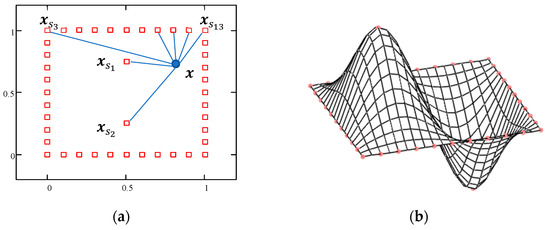
Figure 1.
RBF interactions between source points (a) and surrounding volume (b).
A linear system with an order equal to the number of source points introduced, needs to be solved for the calculation of coefficients . A radial basis fit exists if the coefficients and the weights of the polynomial can be found such that the two following conditions are satisfied:
- The value of assumes the desired value at the point :
- The system is completed if the orthogonality condition of the polynomial terms is verified for all polynomials p with a degree less or equal to that of polynomial :
A unique interpolant exists if the basis function is a conditionally positive definite function. The minimal degree of the correction polynomial depends on the choice of the basis function (a table of polynomial augmentations is reported in [31]). If the basis functions are conditionally positive definite of order , a linear polynomial can be used. The subsequent exposition will assume that the aforementioned hypothesis is valid. A consequence of using a linear polynomial is that rigid body translations are exactly recovered. In a 3D space, the linear polynomial has the form of
The orthogonality conditions of Equation (3) can be expressed as:
The values for the weights of RBF vector and the coefficients vector of the linear polynomial can be obtained by solving the system obtained by imposing the conditions of Equations (2) and (5), which are compactly expressed as:
where are the known values of the interpolating function at the source points and are the coefficients of the polynomial . is the interpolation matrix defined by calculating all of the radial interactions between the source points
is a constraint matrix that arises when balancing the polynomial contribution
Radial basis interpolation works for scalar fields, but the fit can be repeated many times using the same interpolation and constraint matrixes. In this case, the vector is replaced by a rectangular matrix and solved in a column-wise fashion, computing the coefficients and related to each column. If a deformation vector field has to be fitted, each component of the displacement prescribed at the source points is interpolated as follows:
The RBF fit guarantees the passage of the interpolated function through all the points of the original dataset with the prescribed value. The behavior (and smoothness) of the function between points (interpolation) or outside the dataset (extrapolation) depends on the radial function used. Several formulations exist in the literature. Typical RBFs, with global and compact support, are listed in Table 1.

Table 1.
Radial basis functions with global and compact support.
When global support is used, the probe point interacts with all of the points of the cloud, and very high accuracy is achieved. The numerical problem becomes very challenging because a dense, fully populated interpolation matrix has to be solved in the fit stage. Each RBF evaluation requires interaction with all of the sources. Fast methods can be used to accelerate both the fit process and the evaluation of global supported RBF but only for specific cases. The Fast Multipole Method (FMM) is very well established for poly-harmonic splines [32]. The method is based on the concepts of the far and near field. It consists of approximating the evaluation of the interpolating function , considering just a few points close to the probe (near field). The effect of the remaining points (far field) is included by adding a function defined by substituting the cluster of points with an analytical expression that is independent of the number of points (Multipole Expansion). Further details about the adoption of FMM to accelerate the computation of an RBF problem are reported in [33].
Compact supported RBFs are used when long-distance interaction is not desired. The interaction radius can be defined. The Wendland functions with different continuity classes are collected in [34]. The function is active only inside the sphere, identified by the interaction radius , while it is zero outside. It is worth noticing that the compact support affects not only the interpolation behavior but it can also simplify the fitting process as the interpolation matrix of the system becomes sparse and can be managed with numerical algorithms specifically conceived for this class of problems.
Solving large RBF problems requires a high computational cost. Nevertheless, it is suitable for a very efficient parallel implementation. Once the solution is known and shared in the memory of each cluster node, in fact, each partition can smooth its nodes without taking care of what happens outside (high scalability), implicitly guaranteeing the continuity at the interfaces. The acceleration achieved can be really very high (close to 100% efficiency) because the main cost is due to the evaluation of the inter-distance of the points (square root computation). Such a cost can be avoided by implementing specific algorithms in which space partitioning is used to rearrange the problem as the combination of sub-problems adopting Partition of Unity Methods (POU) or using the aforementioned expansion of the far field by Fast Multipole Methods (FMM). The reader can find further details regarding parallel implementations of RBF solutions in [33], including a benchmark on the acceleration achieved with parallel-solving technology.
3. Tools and Procedure Implementation
The procedure implemented consists of a fully automatic analysis workflow suitable to be called within a numerical optimization environment. The parameterization of the geometric model is based on the integration between a morpher tool and a CAE solver accessing and displacing the nodes of the grid from the solver environment. The proposed approach can be adapted to any CAE environment by combining a morpher, a solver, and proper shape update paradigms. In this paper, we demonstrate it for two CAE tools: Simcenter STAR-CCM+ (version 16.02.009-R8), commercialized by Siemens Digital Industries Software (5800 Granite Parkway Suite 600 Plano, TX 75024, United States) and RBF Morph (version 1.9), commercialized by RBF Morph S.R.L. (Via Rosmini 4, 00077 Montecompatri, Rome, Italy). The languages adopted to develop the scripts managing the workflow are C++, Java, and MS-DOS. A brief description of the two solvers adopted follows.
3.1. RBF Morph
The geometric parametrization based on RBF mesh morphing consists of implementing shape modifiers of the computational domain, defining the displacement of a set of source points to be propagated to the volume mesh by adopting the mathematical framework described in Section 2. Its industrial implementation poses two challenges: the numerical complexity related to the solution of the RBF problem for a large number of centers and the definition of suitable paradigms to control the shapes by using RBF effectively. The RBF Morph software allows dealing with both as it comes with a fast RBF solver capable of fitting a large dataset (hundreds of thousands of RBF points can be fitted in a few minutes) and with a suite of modeling tools that allow the user to set up each shape modification in an expressive and flexible way.
RBF Morph was born as an add-on for ANSYS Fluent, which is fully integrated into the solving process. It provides a Graphical User Interface (GUI) to drive the complete setup, solving, and meshing morphing process and a set of commands available from the Text-based User Interface (TUI) to implement automatic procedures. Today, RBF Morph is also available as a standalone library that can be coupled with any code. Its GUI provides tools to extract and control points from the surfaces and edges, to put points on primitive shapes (boxes, spheres, and cylinders), or specify them directly by individual coordinates and displacements. Primitive shapes can be combined in a Boolean form, limiting the action of the morpher itself. The shape information coming from an individual RBF setup is generated interactively and is used subsequently in batch commands that allow the combination of many shape modifications in a non-linear manner. The displacement of the prescribed set of source points can be updated according to the parameters that constitute the parametric space of the model (i.e., the amount of translation, rotation, scaling, and offset prescribed). Every kind of mesh element type (tetrahedral, hexahedral, polyhedral, prismatic, non-conformal interfaces, etc.) is supported.
The definition and the execution of a morphing action are completed in three steps: Setup, Fitting, and Smoothing. The first step is taken by using the software GUI and consists of the manual definition of the RBF problem (select the source points and prescribe the parameters to drive the shape deformation). Fitting is the action in which the RBF system is solved for the prescribed values of the input parameters. The smoothing process is the morphing phase of the mesh. It is performed by applying the prescribed displacement to the grid surfaces and then smoothly propagating the deformation to the surrounding domain volume.
3.2. STAR-CCM+
Simcenter STAR-CCM+ is a Multiphysics Computational Fluid Dynamics (CFD) software. It was first developed by CD-adapco and was acquired by Siemens Digital Industries Software in 2016. It is able to solve problems involving flow (of fluids or solids), heat transfer, and stress, including solid continuum mechanics within a single integrated user interface. The simulation environment includes tools to import and create geometries, generate meshes, solve the governing equations and post-process the results. The software allows the automation of the simulation workflows for design exploration studies and the connection to other CAE software for co-simulation analysis. A key feature is the capability to receive input instructions by API (Application Programming Interface) functionality. Custom UDFs can manage input and output information from the solver. This feature was exploited in this work, creating a UDF that allows for appropriately modifying the geometries by updating the coordinates of the grid vertices.
3.3. Automatic CAE Analysis
STAR-CCM+ allows for the use of user codes to customize the functions written in a compiled language. The user code takes the form of one or more user libraries, each of which contains one or more user functions. Once a user library has been attached, its functions are made available for use in drop-down lists. Functions and library registration functions can be coded in any language, as long as that language is able to bind C-like functions or Fortran subroutines. C++ was here used to write the UDFs that guide the mesh-morphing action within the solver environment. The functions were compiled and linked together, generating a Dynamic Linked Library (DLL) that was to be loaded into STAR-CCM+ and made accessible to the simulation file.
The development of the automatic analysis procedure is performed by several preliminary manual setups and by implementing a set of scripts that control the actions of the analysis. The first step consists of defining the shape parameters, whose intensities will constitute the variable space of the optimization problem. The RBF setup is performed by the RBF Morph user interface adopting the baseline CFD mesh to support the selection of the source points and their movements. The displacements of the points of all of the defined shape modifiers are stored in files to be made available to the procedure. The RBF input files, together with the coordinates of the baseline mesh, fed a UDF, which processes the information, makes the calls to the RBF Morph libraries, and generates the coordinates corresponding to the deformed geometry within the STAR-CCM+ solver. A custom Java Macro is in charge of updating the solver setup, running the CFD analysis, and exporting the solutions. The workflow is guided by an MS-DOS batch procedure that automates the entire parametric analysis. The workflow is schematically represented in Figure 2.
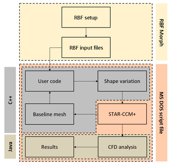
Figure 2.
Flowchart of the automated analysis workflow.
The C++ UDF, which is the core of the procedure, performs the following actions:
- Reads the data stored in the morphing input files: the coordinates and displacements of the RBF centers (referred to as the supporting mesh) are read by the code and stored in a dynamic array;
- Purges nonessential source points: the code makes a call to the RBF Morph “Purge” function, which checks the source points stored in the array and discards those that are below a certain minimum distance from the nearby points;
- Solves the RBF problem: source point coordinates and displacements are provided as arguments to the “Solve” function, which solves the RBF problem;
- Reads the data stored in the baseline mesh file: the coordinates of the vertices (referred to as the baseline mesh built inside of STAR-CCM+) are also read and memorized in a dynamic array;
- Mesh smoothing: the baseline mesh coordinates are fed to the “Morph” function, and the mesh morphing is completed;
- Writes the new coordinates of the mesh into files: the mesh nodes coordinates resulting from the morphing process are stored on a new file.
The operation of reading the baseline mesh is made possible by a previous export of the coordinates of the volume mesh within STAR-CCM+. This is performed by means of the software’s API features, which allow the user to visit the nodal positions of all vertices of the volume mesh.
4. Application to Case Studies
The defined workflow was first applied to a simplified optimization problem, to preliminarily evaluate and, if needed, tune the procedure, and then to a more complex industrial design problem. The first case concerns the aerodynamic optimization of the ASMO (Aerodynamics Studien Model) idealized car body shape. The second application, developed with the collaboration of Volvo Cars, is the identification of a geometry that minimizes the thickness of the water fluid film layer accumulated on the lens of a camera mounted below the side-view mirror.
The objective of the tests was to evaluate the performance of the implemented parameterization tool. For this reason, the attention was oriented to the selection of test cases that include the complexities of problems of practical interest but limited the computational costs by adopting light numerical configurations (coarse meshes). An accurate numerical configuration for the analysis of the side-view mirror was developed by Volvo by adopting a fine mesh. Its solutions are confidential and cannot be reported.
4.1. ASMO Optimization
ASMO geometry is a model created by Daimler-Benz in the ‘90 s to investigate low-drag bodies in automotive aerodynamics and test CFD codes. Wind tunnel experiments were conducted by both Daimler-Benz and Volvo [35]. The shape consists of a square-back rear, smooth surfaces, a boat tail, and an underbody diffuser (Figure 3).
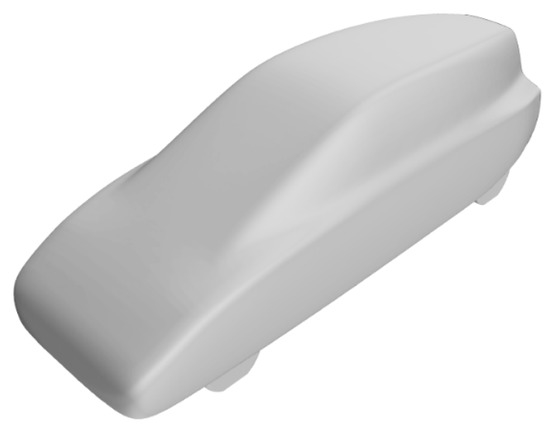
Figure 3.
ASMO geometry.
4.1.1. Shape Parameterization
Three shape modifiers (Figure 4) were selected following previous experience and guidelines [36]. The regions subjected to shape modification were the boat tail, the roof drop, and the front spoiler. The boat tail parameter acts on the lower rear end of the vehicle. The shape variation is performed by rigidly translating the RBF centers located on the left and right edges of the car back. Figure 4a displays the selected source points and their displacement. The range of variation was −10 mm in the inner direction and +20 mm in the outer. The other regions of the mesh (boundaries surfaces and volume) smoothly adapt to the imposed geometry modification according to a globally supported bi-harmonic RBF. The roof drop parameter acts on the rear end of the vehicle. It controls the height of the rear roof, moving up or down a set of RBF centers, as shown in Figure 4b. The range of variation was from −20 mm to +10 mm. A similar parameterization was adopted for the front spoiler shape, which is controlled by moving a set of the RBF centers selected in the front region of the surface. In this case, the displacement direction is oriented with an angle of 20° with respect to the vertical axis (Figure 4c). The lower and upper limits for the variation of this parameter were, respectively, −2.5 mm and +20 mm.
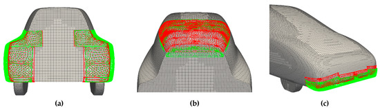
Figure 4.
Boat tail (a), roof drop (b) and front spoiler (c) shape modifiers of the ASMO geometry.
4.1.2. Numerical Configuration and Results
The CFD configuration consisted of steady incompressible RANS (Reynolds-Averaged Navier–Stokes) analyses performed on a mesh modeling half domain, extended two and a half car lengths upstream and six and a half downstream (Figure 5a). A mesh slighter larger than 1.1 million elements was generated. An eight-layer O-Grid was generated on the body wall. A mesh refinement was created in the car wake region spanning approximately 60% of the car length and spreading with an angle of 20° (Figure 5b).
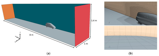
Figure 5.
Dimension of the ASMO numerical domain (a) and details of the grid (b).
The analyses were performed with an inlet flow velocity of 50 m/s. A segregated flow solver and a two-equations k-ε turbulence model have been employed. The convection scheme was the second-order upwind. Wall functions were adopted to model the boundary layer. Two optimization objectives were defined: the minimization of the total drag coefficient of the vehicle and the maximization of the downforce (identified by the inverse of the lift). A DoE (Design of Experiments) table, populated with 25 design points selected adopting an Optimal Space-Filling algorithm [37], was generated. The parameters of the design points are reported in Appendix A in Table A1.
Figure 6 reports the solutions of the analyses. The drag is reported in the abscissa and the lift in the ordinate. The non-dominated solutions, representing the Pareto front, among which to select the optimum compromise, are reported in green, while the baseline solution is represented by a red circle. Two solutions that improve the performance both in terms of drag and lift are identifiable and are indicated by the two arrows in Figure 6. The one with the lowest drag was selected as the optimum solution.
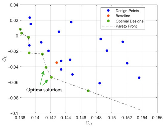
Figure 6.
Solution of the multi−objective ASMO optimization.
Figure 7 reports the comparison between the velocity streamlines visualized on the baseline geometry (Figure 7a) and on the selected optimum (Figure 7b). It is clear that the effect of the reduction in the separated region has a direct effect on aerodynamic drag.
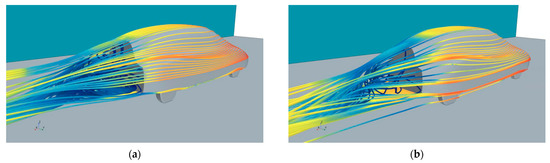
Figure 7.
Comparison between baseline (a) and selected optimum (b) solution for the ASMO model.
The whole workflow was very robust. No failures arose in the script execution or in the mesh morphing actions. The runs were performed on a four-core 1.8 GHz PC equipped with 8 giga of RAM. The complete DoE table was computed in less than 20 h (47.3 min per design points).
4.2. Volvo Car Side-View Mirror
Self-driving vehicles rely on a variety of sensors to gather data and make logical decisions. Because the road infrastructure is constructed for human visual sensors, cameras will continue to be one of the most important sensors. In adverse environmental conditions such as rain, fog, snow, and other forms of severe weather, the quality of computer vision algorithms degrades dramatically. This is aggravated when the camera lens is exposed to rain or to freezing winter conditions. The workflow described in this paper was applied to modify the shape of geometric details around a camera mounted on the underside of a Volvo side-view mirror. The objective is to minimize the thickness of the fluid film that is deposited on the lens.
4.2.1. Baseline Numerical Model
The model of the side-view mirror, with the camera mounted beneath, is attached to the DrivAer model [38] (Figure 8), which is a generic car model developed at the Institute of Aerodynamics and Fluid Mechanics of the Technische Universität München. The numerical domain is similar to the domain generated for the ASMO test case, with similar proportions to the far-field location with respect to the model. Two overlapping meshes were generated: a coarse grid around the vehicle, adopted as background mesh, and a finer one in a small volume around the mirror to be used as overlapping. The dimensions of the meshes were about one million cells for the background and almost two hundred thousand for the overlapping one.
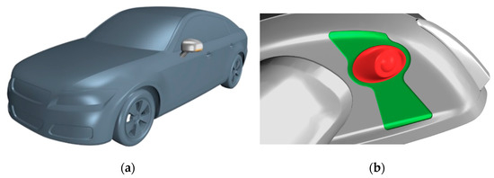
Figure 8.
DrivAer car model (a) and detail of Volvo side mirror (b).
As it is a configuration in which both air and water share the same numerical domain, a multiphase analysis is required. The flow is initialized with a single-phase analysis in stationary conditions. A restart is then performed, activating a transient multiphase (air/fluid film) configuration solving one second with a time step of 0.001 sec. In the second stage, additional boundary conditions are imposed, including the definition of a shell region (affecting a two-dimensional one-cell-thick region of space with edges and boundaries) that represents the space within which the fluid film flows (Figure 9a) and a fluid film inlet/outlet system (Figure 9b). The Eulerian Multiphase (EMP) Fluid Film model provides a mathematical description of the behavior of the water film, allowing the specification of an inlet from which the fluid film is emitted and an outlet from which it is removed.
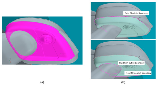
Figure 9.
Shell region created on the underside of the mirror (a) and inlet/outlet system through the shell region (b).
The model assumes that the film is thin enough to be approximated by the laminar boundary layer approximation. To calculate the liquid film thickness on the underside of the mirror, the continuity equation that governs the conservation of mass within the shell region was used:
where and represent, respectively, the density and the velocity of the fluid film. The quantity represents the source term of the mass of fluid film per unit area. The initial thickness of the fluid film on the shell region was set to 0.1 mm. Water flows from the inlet boundary with a 0.5 mm thickness and a velocity of 4.36 mm/s. As it flows down the shell region, the water is affected by both air flow around the vehicle and gravity, forming a liquid film in the process. In some cases, the film thickness can become very large. It happens, for example, when the liquid film is pushed into a corner, and it cannot escape. A limit on the maximum thickness was imposed. When the specified thickness of 1 mm is reached, any extra fluid is removed from the film. Moreover, for this case, the two-equations k-ε turbulence model was adopted to solve the boundary layer by wall functions.
4.2.2. Mirror Shape Parameterization
The parameterization of the geometry must respect the constraint of maintaining an unchanged camera installation and the shape of its support (red region of Figure 8b). Moreover, the top part of the mirror must be kept unchanged. The geometry that can be subjected to modification is limited to the pocket located on the bottom of the mirror in a region around the support of the camera (green region of Figure 8b).
Six shape modifiers were defined. Three of them act on the straight borders of the pocket, rotating the points around the start of the segments (Figure 10a). Two parameters act on the curved sides, scaling the shapes with respect to the center of the pocket (Figure 10b). The last parameter controls the depth of the pocket (Figure 10c).
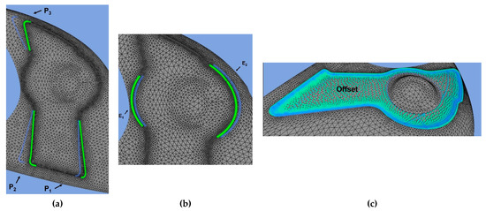
Figure 10.
Parameterization of the mirror geometry acting on the straight borders (a), on the curved sides (b) and on the pocket (c).
4.2.3. Optimization Results
The objective function of the optimization was the mean fluid film thickness deposited on the camera lens, which coincides with the small spherical portion visible in the middle of the red region highlighted in Figure 8b. With the view of this optimization example to be a test for the implemented workflow, only 25 candidates were selected (adopting an Optimal Space-Filling algorithm) to populate a DoE table. Table A2 in Appendix A reports the maximum displacements of the source points controlled by each parameter.
The workflow was demonstrated to be very robust also in this case despite the occurrence of two failures due to a combination of parameters that involved an extreme geometric variation, which was not compatible with the generated mesh. Figure 11 reports the solutions of the analyses. Among the list of candidates, it is possible to select a design configuration that reduces the mean fluid film thickness accumulated on the camera lens by about 40% with respect to the baseline.
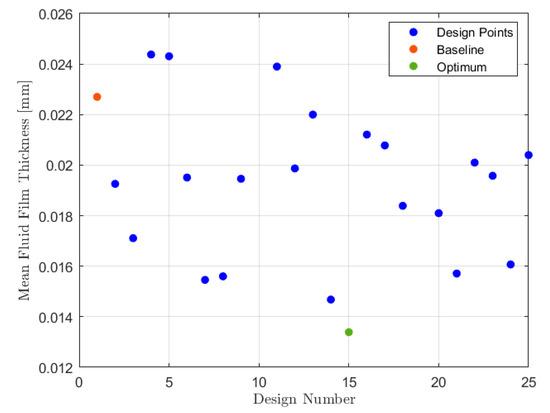
Figure 11.
Solution of the Volvo mirror optimization.
Figure 12 compares the baseline solution with the optimum one. The thickness of the average fluid film accumulated on the surface is represented in blue.
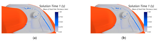
Figure 12.
Average fluid film thickness deposition for the baseline (a) and optimum geometry (b).
A better solution might be identified by relaxing some constraints and/or refining the optimization strategy (richer DoE table or appropriate decision-making algorithm), but this was not the focus of this activity. The objective of this application was to test the integration between the mesh morphing tool and the CAE solver, verify the efficiency of the implemented procedure, and to test the robustness of the workflow in a complex industrial setup. From this point of view, the tests demonstrated the potentialities of the methodology and supported the identification of opportune development strategies to improve the tool.
The computations of the Volvo test case were performed on a workstation equipped with two Intel® Xeon® E5-2680 v2 processors (10 cores each), operating at a base frequency of 2.80 GHz and 128 GB of RAM. A single design point evaluation required an average of 45 min. The DoE table was completed in less than 20 h.
5. Conclusions
An automatic parametric CAE analysis workflow based on RBF mesh morphing was developed and tested. The benefit of the proposed methodology is the integration between the mesh morphing and the CAE tool allowing to perform shape modifications by accessing the mesh from the solver environment. The prospect of such a coupling offers several advantages in terms of robustness of the analyses, time to setup, and consistency of the solutions.
The adopted mesh morphing technology is based on the RBF Morph morpher tool, which is already capable of being coupled with several CAE solvers. This paper details the activity performed to extend its coupling capability to the STAR-CCM+ CFD solver opening a path to a strong integration within its environment as it is already available with other codes. The link was implemented by user-defined routines that manage the association of the morpher tool to the mesh available from the analysis code. The objective is to preliminarily test the workflow in the view to refine the integration within the CAE solver. The advantage of this approach, which has a great impact when dealing with large meshes, and the robustness deriving from the incorporation of the morphing action within the solver environment was highlighted. The latter aspect, in particular, offers the opportunity to extend the analysis capability to complex multidisciplinary phenomena.
The workflow was tested on two numerical optimization problems adopted as demonstrators: a simple setup concerning the aerodynamic optimization of the ASMO car body and a complex setup in which to identify a geometry that minimizes the water film accumulation on a camera mounted below a car side mirror. In both cases, the procedure showed to be very robust and to properly manage the mesh made available to the morpher from the CAE solver environment. Furthermore, the work supported the identification of the areas of improvement in the methodology and allowed the definition of the actions to be performed for a strong integration of the RBF Morph technology within the STAR-CCM+ environment.
Author Contributions
Conceptualization, U.C., D.P., S.P. and M.E.B.; methodology, D.P., S.P. and M.E.B.; software, D.P.; formal analysis, D.P.; investigation, D.P.; resources, S.P., T.V. and M.E.B.; data curation, U.C., D.P., S.P., T.V. and M.E.B.; writing—original draft preparation, U.C. and D.P.; writing—review and editing, U.C., D.P., S.P., T.V. and M.E.B.; visualization, D.P.; supervision, M.E.B. All authors have read and agreed to the published version of the manuscript.
Funding
This research received no external funding.
Data Availability Statement
Not applicable.
Conflicts of Interest
One of the authors (Marco E. Biancolini) is the developer and the owner of the commercial software RBF Morph.
Appendix A
Table A1.
DoE table of the ASMO test case.
Table A1.
DoE table of the ASMO test case.
| ID | Boat Tail (Left) [mm] | Boat Tail (Right) [mm] | Roof Drop [mm] | Front Spoiler [mm] |
|---|---|---|---|---|
| 1 | 18.20 | −18.20 | −8.60 | 6.95 |
| 2 | 11.00 | −11.00 | −17.00 | 9.65 |
| 3 | 8.60 | −8.60 | 4.60 | 17.75 |
| 4 | 12.20 | −12.20 | 9.40 | 10.55 |
| 5 | −2.20 | 2.20 | −1.40 | 18.65 |
| 6 | 0.20 | −0.20 | 1.00 | −2.05 |
| 7 | 1.40 | −1.40 | −19.40 | 3.35 |
| 8 | −1.00 | 1.00 | 8.20 | 13.25 |
| 9 | 7.40 | −7.40 | −9.80 | 19.55 |
| 10 | 2.60 | −2.60 | −18.20 | 14.15 |
| 11 | 9.80 | −9.80 | 5.80 | 0.65 |
| 12 | 17.00 | −17.00 | −13.40 | 15.95 |
| 13 | 6.20 | −6.20 | 2.20 | 7.85 |
| 14 | 13.40 | −13.40 | −15.80 | 1.55 |
| 15 | −4.60 | 4.60 | −11.00 | −0.25 |
| 16 | 14.60 | −14.60 | −5.00 | −1.15 |
| 17 | 5.00 | −5.00 | −7.40 | 2.45 |
| 18 | 19.40 | −19.40 | 3.40 | 6.05 |
| 19 | 3.80 | −3.80 | −6.20 | 11.45 |
| 20 | −5.80 | 5.80 | −12.20 | 16.85 |
| 21 | −3.40 | 3.40 | 7.00 | 4.25 |
| 22 | −7.00 | 7.00 | −14.60 | 8.75 |
| 23 | 15.80 | −15.80 | −2.60 | 15.05 |
| 24 | −8.20 | 8.20 | −3.80 | 5.15 |
| 25 | −9.40 | 9.40 | −0.20 | 12.35 |
Table A2.
DoE table of the Volvo test case.
Table A2.
DoE table of the Volvo test case.
| ID | P1 [mm] | P2 [mm] | P3 [mm] | E1 [mm] | E2 [mm] | Offset [mm] |
|---|---|---|---|---|---|---|
| 1 | 0.70 | 14.70 | 3.90 | −0.36 | 1.72 | 0.37 |
| 2 | −4.10 | 2.10 | 6.90 | −0.44 | 0.52 | 0.41 |
| 3 | 6.10 | 5.70 | 5.70 | −0.04 | 2.92 | 0.39 |
| 4 | 1.30 | 8.70 | 14.70 | −0.68 | 2.68 | 0.45 |
| 5 | −1.70 | 1.50 | 2.10 | −1.64 | −0.20 | 0.19 |
| 6 | 9.70 | 12.90 | 9.30 | −0.60 | 0.28 | 0.13 |
| 7 | −1.10 | 7.50 | 2.70 | −0.28 | 0.76 | 0.03 |
| 8 | −0.50 | 14.10 | 10.50 | −0.92 | 3.16 | 0.09 |
| 9 | 8.50 | 10.50 | 9.90 | −1.48 | 3.64 | 0.31 |
| 10 | 7.30 | 12.30 | 0.30 | −1.56 | 1.00 | 0.25 |
| 11 | 5.50 | 3.90 | 7.50 | −1.08 | −1.88 | 0.05 |
| 12 | 4.90 | 2.70 | 4.50 | −1.72 | 1.24 | 0.47 |
| 13 | −2.90 | 13.50 | 5.10 | −1.32 | −1.16 | 0.17 |
| 14 | 3.10 | 5.10 | 12.90 | −0.12 | 1.96 | 0.07 |
| 15 | −4.70 | 4.50 | 13.50 | −1.16 | 0.04 | 0.15 |
| 16 | 7.90 | 0.90 | 11.70 | −0.76 | −0.44 | 0.33 |
| 17 | −3.50 | 9.90 | 8.10 | −1.80 | 1.48 | 0.43 |
| 18 | 4.30 | 9.30 | 14.10 | −1.88 | −0.68 | 0.21 |
| 19 | 2.50 | 8.10 | 6.30 | −1.96 | 2.20 | 0.01 |
| 20 | −2.30 | 6.90 | 1.50 | −1.00 | 3.88 | 0.27 |
| 21 | 0.10 | 11.10 | 12.30 | −0.20 | −1.40 | 0.29 |
| 22 | 3.70 | 6.30 | 0.90 | −0.52 | −1.64 | 0.35 |
| 23 | 6.70 | 11.70 | 8.70 | −1.24 | −0.92 | 0.49 |
| 24 | 9.10 | 3.30 | 3.30 | −0.84 | 2.44 | 0.11 |
| 25 | 1.90 | 0.30 | 11.10 | −1.40 | 3.40 | 0.23 |
References
- Poli, C. Design for Manufacturing: A Structured Approach, 1st ed.; Butterworth-Heinemann, Reed Elsevier Group: Oxford, UK, 31 August 2001. [Google Scholar]
- Shah, J.J. Assessment of features technology. Comput. Aided Des. 1991, 23, 331–343. [Google Scholar] [CrossRef]
- Woodbury, R. Elements of Parametric Design; Routledge: London, UK, 2010. [Google Scholar]
- Camba, J.D.; Contero, M.; Company, P. Parametric CAD modeling: An analysis of strategies for design reusability. Comput. Aided Des. 2016, 74, 18–31. [Google Scholar] [CrossRef]
- Hardee, E.; Chang, K.H.; Tu, J.; Choi, K.K.; Grindeanu, I.; Yu, X. A CAD-based design parameterization for shape optimization of elastic solids. Adv. Eng. Softw. 1999, 30, 185–199. [Google Scholar] [CrossRef]
- Kodiyalam, S.; Kumar, V.; Finnigan, P.M. Constructive solid geometry approach to three-dimensional structural shape optimization. AIAA J. 1992, 30, 1408–1415. [Google Scholar] [CrossRef]
- Agarwal, D.; Robinson, T.T.; Armstrong, C.G.; Kapellos, C. Enhancing CAD-based shape optimisation by automatically updating the CAD model’s parameterisation. Struct. Multidiscip. Optim. 2019, 59, 1639–1654. [Google Scholar] [CrossRef]
- Storti, B.; Garelli, L.; Storti, M.; D’Elía, J. Optimization of an internal blade cooling passage configuration using a Chimera approach and parallel computing. Finite Elem. Anal. Des. 2020, 177, 103423. [Google Scholar] [CrossRef]
- Skinner, S.N.; Zare-Behtash, H. State-of-the-art in aerodynamic shape optimisation methods. Appl. Soft Comput. 2018, 62, 933–962. [Google Scholar] [CrossRef]
- Samareh, J.A. Survey of Shape Parameterization Techniques for High-Fidelity Multidisciplinary Shape Optimization. AIAA J. 2001, 39, 877–884. [Google Scholar] [CrossRef]
- Rousseau, Y.; Men’shov, I.; Nakamura, Y. Morphing-based shape optimization in computational fluid dynamics. Trans. Jpn. Soc. Aeronaut. Space Sci. 2007, 50, 41–47. [Google Scholar] [CrossRef][Green Version]
- Masud, A.; Bhanabhagvanwala, M.; Khurram, R.A. An Adaptive Mesh Rezoning Scheme for Moving Boundary Flows and Fluid-Structure Interaction. Comput. Fluids 2007, 36, 77–91. [Google Scholar] [CrossRef]
- de Boer, A.; van der Schoot, M.S.; Bijl, H. Mesh deformation based on radial basis function interpolation. Comput. Struct. 2007, 85, 784–795. [Google Scholar] [CrossRef]
- Saderberg, T.; Parry, S. Free-form deformation of solid geometric models. In Proceedings of the 13th Annual Conference on Computer Graphics and Interactive Techniques, Dallas, TX, USA, 18–22 August 1986; pp. 151–160. [Google Scholar]
- Jakobsson, S.; Amoignon, O. Mesh deformation using radial basis functions for gradient-based aerodynamic shape optimization. Comput. Fluids 2007, 36, 1119–1136. [Google Scholar] [CrossRef]
- Biancolini, M.E.; Biancolini, C.; Costa, E.; Gattamelata, D.; Valentini, P.P. Industrial application of the meshless morpher RBF Morph to a motorbike windshield optimisation, EASC 2009. In Proceedings of the 4th European Automotive Simulation Conference, Munich, Germany, 6–7 July 2009. [Google Scholar]
- Biancolini, M.E. Mesh Morphing and Smoothing by Means of Radial Basis Functions (RBF): A Practical Example Using Fluent and RBF Morph. In Handbook of Research on Computational Science and Engineering: Theory and Practice; IGI Global: Hershey, PA, USA, 2012. [Google Scholar]
- Biancolini, M.E.; Costa, E.; Cella, U.; Growth, C.; Veble, G.; Andrejašič, M. Glider Fuselage–Wing Junction Optimization using CFD and RBF Mesh Morphing. Aircr. Eng. Aerosp. Technol. J. 2016, 88, 740–752. [Google Scholar] [CrossRef]
- Growth, C.; Costa, E.; Biancolini, M.E. RBF-based mesh morphing approach to perform icing simulations in the aviation sector. Aircr. Eng. Aerosp. Technol. 2019, 91, 620–633. [Google Scholar] [CrossRef]
- Biancolini, M.E.; Cella, U. Radial Basis Functions Update of Digital Models on Actual Manufactured Shapes. ASME J. Comput. Nonlinear Dyn. 2019, 14. [Google Scholar] [CrossRef]
- Cella, U.; Groth, C.; Porziani, S.; Clarich, A.; Franchini, F.; Biancolini, M.E. Combining Analytical Models and Mesh Morphing Based Optimization Techniques for the Design of Flying Multihulls Appendages. J. Sail. Technol. 2021, 6, 151–172. [Google Scholar] [CrossRef]
- Geronzi, L.; Gasparotti, E.; Capellini, K.; Cella, U.; Groth, C.; Porziani, S.; Chiappa, A.; Celi, S.; Biancolini, M.E. High fidelity fluid-structure interaction by radial basis functions mesh adaption of moving walls: A workflow applied to an aortic valve. J. Comput. Sci. 2021, 51, 101327. [Google Scholar] [CrossRef]
- Groth, C.; Chiappa, A.; Porziani, S.; Biancolini, M.E.; Jacoboni, E.; Serioli, E.; Mastroddi, F. Multiphysics numerical investigation on the aeroelastic stability of a Le Mans Prototype car. Procedia Struct. Integr. 2019, 24, 875–887. [Google Scholar] [CrossRef]
- Li, R.; Xu, P.; Yao, S. Optimization of the high-speed train head using the radial basis function morphing method. Proc. Inst. Mech. Eng. Part F J. Rail Rapid Transit 2019, 234, 96–107. [Google Scholar] [CrossRef]
- Felici, A.; Martínez-Pascual, A.; Groth, C.; Geronzi, L.; Porziani, S.; Cella, U.; Brutti, C.; Biancolini, M.E. Analysis of Vortex Induced Vibration of a Thermowell by High Fidelity FSI Numerical Analysis Based on RBF Structural Modes Embedding. In Lecture Notes in Computer Science; Springer: Cham, Switzerland, 2021; Volume 12746. [Google Scholar]
- Porziani, S.; Groth, C.; Waldman, W.; Biancolini, M.E. Automatic shape optimisation of structural parts driven by BGM and RBF mesh morphing. Int. J. Mech. Sci. 2021, 189, 105976. [Google Scholar] [CrossRef]
- Groth, C.; Porziani, S.; Chiappa, A.; Pompa, E.; Cenni, R.; Cova, M.; D’Amico, G.; Giorgetti, F.; Brutti, C.; Salvini, P.; et al. High fidelity numerical fracture mechanics assisted by RBF mesh morphing. Procedia Struct. Integr. 2020, 25, 136–148. [Google Scholar] [CrossRef]
- Biancolini, M.E.; Cella, U.; Groth, C.; Genta, M. Static Aeroelastic Analysis of an Aircraft Wind-Tunnel Model by Means of Modal RBF Mesh Updating. ASCE’s J. Aerosp. Eng. 2016, 29, 04016061. [Google Scholar] [CrossRef]
- Lodha, S.K.; Franke, R. Scattered Data Interpolation: Radial Basis and Other Methods. In Handbook of Computer Aided Geometric Design; North Holland: Amsterdam, The Netherlands, 2002; Chapter 16; pp. 389–404. [Google Scholar]
- Buhmann, M.D. Radial Basis Functions: Theory and Implementations. In Cambridge Monographs on Applied and Computational Mathematics; Cambridge University Press: Cambridge, UK, 2004. [Google Scholar]
- Boyd, P.B.; Gildersleeve, K.W. Numerical experiments on the condition number of the interpolation matrices for radial basis functions. Appl. Numer. Math. 2011, 61, 443–459. [Google Scholar] [CrossRef]
- Beatson, R.K.; Powell, M.J.D.; Tan, A.M. Fast evaluation of polyharmonic splines in three dimensions. IMA J. Numer. Anal. 2007, 27, 427–450. [Google Scholar] [CrossRef][Green Version]
- Biancolini, M.E. Fast Radial Basis Functions for Engineering Applications; Springer: Cham, Switzerland, 2017. [Google Scholar]
- Wendland, H. Piecewise polynomial, positive definite and compactly supported radial basis functions of minimal degree. Adv. Comput. Math. 1995, 4, 389–396. [Google Scholar] [CrossRef]
- Tsubokura, M.; Kobayashi, T.; Nakashima, T.; Nouzawa, T.; Nakamura, T.; Zhang, H.; Onishi, K.; Oshima, N. Computational visualization of unsteady flow around vehicles using high performance computing. Comput. Fluids 2009, 38, 981–990. [Google Scholar] [CrossRef]
- Lietz, R.L. Vehicle Aerodynamic Shape Optimization. SAE Int. 2011. [CrossRef]
- Wang, X.; Tsung, F.; Li, W.; Xiang, D.; Cheng, C. Optimal space-filling design for symmetrical global sensitivity analysis of complex black-box models. Appl. Math. Model. 2021, 100, 303–319. [Google Scholar] [CrossRef]
- Heft, A.I.; Indinger, T.; Adams, N.A. Experimental and Numerical Investigation of the DrivAer Model. In Proceedings of the ASME 2012 10th International Conference on Nanochannels, Microchannels, and Minichannels, Rio Grande, PR, USA, 8–12 July 2012; Volume 1: Symposia, Parts A and B, pp. 41–51. [Google Scholar]


Publisher’s Note: MDPI stays neutral with regard to jurisdictional claims in published maps and institutional affiliations. |
© 2022 by the authors. Licensee MDPI, Basel, Switzerland. This article is an open access article distributed under the terms and conditions of the Creative Commons Attribution (CC BY) license (https://creativecommons.org/licenses/by/4.0/).