Article

Phase Convergence and Crest Enhancement of Modulated Wave Trains

1
School of Engineering, The University of Tokyo, Bunkyo, Tokyo 113-8656, Japan
2
Fluids Engineering and Ship Performance Evaluation Department, National Maritime Research Institute, Mitaka, Tokyo 181-0004, Japan
3
Graduate School of Frontier Sciences, The University of Tokyo, Kashiwa, Chiba 277-8563, Japan
*
Author to whom correspondence should be addressed.
Fluids 2022, 7(8), 275; https://doi.org/10.3390/fluids7080275
Submission received: 17 July 2022 / Revised: 5 August 2022 / Accepted: 7 August 2022 / Published: 11 August 2022
(This article belongs to the Special Issue Nonlinear Wave Hydrodynamics, Volume II)

Abstract

:
The Akhmediev breather (AB) solution of the nonlinear Schrödinger equation (NLSE) shows that the maximum crest height of modulated wave trains reaches triple the initial amplitude as a consequence of nonlinear long-term evolution. Several fully nonlinear numerical studies have indicated that the amplification can exceed 3, but its physical mechanism has not been clarified. This study shows that spectral broadening, bound-wave production, and phase convergence are essential to crest enhancement beyond the AB solution. The free-wave spectrum of modulated wave trains broadens owing to nonlinear quasi-resonant interaction. This enhances bound-wave production at high wavenumbers. The phases of all the wave components nearly coincide at peak modulation and enhance amplification. This study found that the phase convergence observed in linear-focusing waves can also occur due to nonlinear wave evolution. These findings are obtained by numerically investigating the modulated wave trains using the higher-order spectral method (HOSM) up to the fifth order, which allows investigations of nonlinearity and spectral bandwidth beyond the NLSE framework. Moreover, the crest enhancement is confirmed through a tank experiment wherein waves are generated in the transition region from non-breaking to breaking. Owing to strong nonlinearity, the maximum crest height observed in the tank begins to exceed the HOSM prediction at an initial wave steepness of 0.10.

1. Introduction

Rogue waves (or freak waves) in the ocean can cause major damage to ships and offshore structures. A number of tank experiments have been conducted to examine such strongly nonlinear and complicated interactions of rogue waves with ships and offshore structures [1,2,3,4,5]. The occurrence probability of such waves may need to be taken into account when designing or establishing rules for ships and offshore structures [6,7]. In addition to the occurrence probability, the shape of rogue waves affects the maximum wave load acting on ships [4]. The crest height of rogue waves is also of great concern for fixed offshore platforms because an air gap is the height between the wave crest and the platform deck [8,9].
Recent studies have revealed that modulational instability due to quasi-resonant interaction is one of the causes of rogue-wave formation [10,11,12]. Many studies have been conducted on the modulational instability or quasi-resonant interaction of water waves, starting from the discovery that Stokes waves are unstable under sideband modulations [13,14]. Such nonlinear wave evolutions are governed by the balance between nonlinearity and dispersion. This balance is expressed as a ratio between the wave steepness and spectral bandwidth (e.g., δ ^ for modulated wave trains [15] and the Benjamin–Feir index (BFI) for irregular waves [10]). The ratio δ ^ affects the initial growth of unstable sidebands [13], the recurrence period [16], and the maximum amplitude or crest height [17,18,19,20] of modulated wave trains. Moreover, the BFI is a key parameter for the occurrence probability of rogue waves [10,21].
This study focuses on the maximum crest height of modulated wave trains, or the maximum amplification of modulated wave trains, which is defined as the ratio between the maximum crest height and the initial Stokes-wave amplitude. This has been addressed in several experimental [22,23] and numerical [23,24,25] studies. Su and Green [22] and Tanaka [24] investigated the variation in maximum amplification against initial wave steepness. Through numerical simulation, Tanaka [24] showed that the maximum amplification predicted by the nonlinear Schrödinger equation (NLSE) [26] and a two-dimensional fully-nonlinear (FNL) potential flow solver [27] was much higher than the experimental results of Su and Green [22]. Tanaka’s FNL simulation also showed that the maximum amplification could exceed 3 depending on the initial wave steepness. On the basis of experimental results and numerical results from the Dysthe equation [28], Waseda [23] showed that the difference between the numerical results of Tanaka [24] and the experimental results of Su and Green [22] could be explained, to a certain degree, by the influence of the spectral bandwidth of modulated wave trains. Su and Green [22] and Tanaka [24] determined that the spectral bandwidth had a one-to-one correspondence with the initial wave steepness. However, the maximum amplification can differ significantly depending on the spectral bandwidth for a given initial wave steepness. Slunyaev and Shrira [25] investigated the dependence of the maximum amplification of modulated wave trains on both the initial wave steepness and spectral bandwidth by analyzing the Akhmediev breather (AB) solution of the NLSE [17,29] and performing FNL simulation based on conformal mapping [30]. In this FNL simulation, a maximum amplification larger than 4 was observed in the specific case of a very narrow spectral bandwidth. Waseda [23] pointed out that, for a given initial wave steepness, the maximum amplification increases as the spectral bandwidth narrows. This relation was analytically explained by the AB solution in the cubic NLSE regime [18,19,20,25].
Such work has clarified the significant influence of the initial wave steepness and spectral bandwidth on the maximum crest height of modulated wave trains. However, it is still unclear why the maximum amplification of modulated wave trains can exceed 3, although AB predicts the maximum to be 3 in the limit of zero spectral bandwidth [18,19,20,25]. Therefore, the aim of this study is to clarify the physics behind crest enhancement of modulated wave trains from the spectral-broadening and phase-convergence [31] perspectives. To investigate crest enhancement, tank experiments generating modulated wave trains were carried out and corresponding numerical simulations using the higher-order spectral method (HOSM) [32,33] were performed. The evolution of the spectral broadening and degree of phase convergence were analyzed using the HOSM outputs in the non-wave-breaking regime. Note that the maximum wave height and maximum trough depth are parameters similar to the maximum crest height that this study focuses on. However, for a given modulated wave train, these three values differ [25] because of different bound-wave contributions to them [34].
Section 2 describes the set-up for the numerical simulations and experiments on modulated wave trains. The simulated and experimental results are compared in Section 3. The mechanism of crest enhancement of modulated wave trains is discussed in Section 4, and the conclusions of this study follow in Section 5.

2. Facility and Methods

2.1. Numerical Simulations

The temporal evolution of spatially periodic deep-water modulated wave trains was numerically simulated using the HOSM [32,33] in the same manner as in our preceding studies [35,36]. The HOSM numerically solves Laplace’s equation ( 2 ϕ   =   0 ) subject to nonlinear kinematic and dynamic free-surface boundary conditions with respect to the surface elevation ζ and velocity potential on the free surface, Φ S   =   ϕ z = ζ [26]:
ζ t   +   x ζ · x Φ S     1   +   x ζ · x ζ W   =   0 , Φ t S   +   g ζ   +   1 / 2 x Φ S     1 / 2 1   +   x ζ · x ζ W 2   =   0 ,
where x   =   / x , / y ,   W   =   ϕ / z z   =   ζ , and g denotes the gravitational acceleration. ϕ is expanded in a perturbation series up to an arbitrary nonlinear order M . M   =   3 5 is typically used [37] because the nonlinear wave evolution due to quasi-resonant interaction can be captured with M     3 . In addition to the nonlinear wave evolution, M also governs the accuracy of the bound wave production. Therefore, this study adopted M   =   5 to take into account the bound waves up to the fifth order correctly. The spatial derivatives ( x · ) were solved in wavenumber space using the fast Fourier transform, which enabled efficient calculation. To remove spurious high-frequency waves arising from aliasing, the following low-pass filter proposed in [32] was applied:
k   <   N x M   +   1 d k ,
where k , d k , and N x denote the wavenumber, wavenumber interval, and number of spatial nodes in the x direction, respectively. This study only addressed unidirectional modulated wave trains propagating in the x direction. The HOSM cannot take into account wave breaking directly because the free surface ζ is assumed to be a single-valued function with respect to the horizontal coordinate x . However, when a wave sufficiently steep to break appears in the HOSM simulation, the low-pass filter in Equation (2) removes the energies of high-wavenumber components. Accordingly, the computation can continue to some extent beyond possibly breaking events [38,39].
The initial wave profile of the HOSM simulation was a three-wave system consisting of a carrier, upper sideband, and lower sideband (denoted as c , + , and , respectively) [13,15]:
ζ x   =   a c cos k c x   +   a + cos k + x + ψ +   +   a cos k x   +   ψ ,
where a , k , and ψ denote the amplitude, wavenumber, and phase, respectively. k ± is defined as k c ± δ k , where δ k is the perturbation wavenumber. Table 1 lists the parameters of the initial wave profiles of the modulated wave trains used in the HOSM simulation. The perturbation wavenumber δ k / k c   =   1 / 7 was selected because the crest amplification was expected to exceed 3 at large wave steepness from the FNL simulation results in [25]. While δ k / k c , representing the spectral bandwidth, was fixed, the initial wave steepness a 0 k c was swept between 0.08 and 0.115. This a 0 k c range was selected based on [15,25] to cover the transition region from non-breaking to breaking in the tank. The critical parameter δ ^ introduced in Section 1, which governs the nonlinear evolution of modulated wave trains [15], is given by
δ ^   =   1 2 δ k / k c a 0 k c
and was systematically varied from 0.62 to 0.89. The amplitude ratio of the sidebands to the Stokes wave a ± / a 0 was fixed to 0.1 sufficiently smaller than 1 such that the sidebands grow exponentially [13]. The initial sideband phases ϕ ± was set to π / 4 , which gives the maximum sideband growth rate [13].
The initial wave profile (Equation (3)) was given on the basis of linear wave theory and did not satisfy the fully nonlinear free-surface boundary condition (Equation (1)). Therefore, this study adopted the nonlinear-wave initialization method proposed in [40] (see also [36]). The initially linear wave field was gradually transformed into a nonlinear wave field with an adjustment period T a . T a   =   32 T c , where T c denotes the period of the carrier wave.
An example wave-elevation time-series of modulated wave trains with a 0 k c   =   0.08 is presented in Figure 1a. The modulation of the wave group evolves gradually, and the maximum crest appears at the peak of the modulation ( t   =   t m a x   =   228   s ). Then, the wave group begins to demodulate afterward, and almost the initial wave profile is recovered ultimately. Such a full cycle of recurrence [15] is confirmed to be successfully captured by the HOSM simulation.

2.2. Tank Experiment

A wave-generation experiment was performed in a wave tank (WT) (50 m × 8 m × 4.5 m) (Figure 2) at the National Maritime Research Institute (Tokyo, Japan) to compare its results with those of the HOSM simulation and to investigate modulated wave trains including wave breaking. The modulated wave trains were generated using the HOSM wave generation (HOSM-WG) method [36]. A nonlinear wave field precomputed with the HOSM was generated in a wave tank by sending a temporally evolving signal calculated from the HOSM output to a wave maker. HOSM-WG can control when and where the maximum crest height appears in a wave tank. In this study, the modulated wave trains were generated such that the maximum crest appeared at t   =   40 s after the beginning of wave generation and at x   =   12 m from the wave maker in the WT.
A capacitance wave gauge was set at x   =   12 m to measure the wave-elevation time series. However, the location of the maximum crest could deviate from x   = 12 m, especially when wave breaking occurred. To measure the maximum crest height even in cases of wave breaking, the wave-surface profiles were measured using a stereo-imaging technique [4,41]. About 100 spherical floats with a diameter of less than 20 mm were set on the wave surface, and two cameras tracked the three-dimensional motion of these floats. The wave profiles were acquired by fitting a smoothing spline curve to the floats’ three-dimensional coordinates [4], and the maximum crest height was evaluated. The set-up of the stereo cameras in the WT is illustrated in Figure 2, where the measurement area is also indicated. The estimated error in the crest height of regular waves with a wavelength of 3 m and wave height between 10 and 20 cm is less than 4% in this stereo-imaging scheme [41]. Note that the standard deviation of the wave-maker motion was found to be 1.065 times larger than the given signal owing to a problem with controlling the mechanical wave maker [35]. Therefore, the experimental results presented in Section 3 are corrected by a factor of 1.065 for comparison with the HOSM simulation.
The generations of modulated wave trains with the HOSM-WG in a tank were validated with HOSM simulation, as reported in [36,42]. Here, as an example, the comparison of the wave elevation of the modulated wave train with a 0 k c   =   0.08 between the HOSM-WG in the WT and the corresponding HOSM output is presented in Figure 1b. The mean square error between those wave-elevation time series in the range with T g / 2     t     t m a x     T g / 2 is 0.87 % of the total energy ( a 0 2 / 2 ). Here, T g   =   2 T c k c / δ k = 14 T c denotes the wave-group period, and this time range is indicated as vertical dashed lines in Figure 1b. In this way, the modulated wave train simulated in the HOSM simulation can be well reproduced in the WT. However, the primary focus of this study is the strong nonlinearity at large a 0 k c in the physical tank that cannot be considered in the HOSM simulation. Such a strongly nonlinear influence on the crest enhancement of modulated wave trains, causing some differences between the HOSM-WG in the tank and HOSM-simulation, will be demonstrated in Section 3.

3. Results of Numerical Simulations and Experiments

In this section, the maximum crest heights of the modulated wave trains between the HOSM simulation and the WT experiment are compared. Figure 3 presents the variation in the normalized maximum crest height ζ c r / a 0 with the initial wave steepness a 0 k c . For reference, Figure 3 also shows the predictions of the AB solution of the NLSE with and without the second-order bound-wave correction. The maximum crest height of the free wave, ζ c r A B ; f , and that taking into account the bound wave, ζ c r A B ; f   +   b , for the AB solution are given respectively by
ζ c r A B ; f a 0   =   1   +   2 1     1 2 δ ^ 2  
and
ζ c r A B ;   f   +   b a 0   =   ζ c r A B ; f a 0 1   +   1 2 k c ζ c r A B ; f .
These are derived in Appendix A. The definition of δ ^ , expressing the balance between the initial wave steepness and spectral bandwidth, is given in Equation (4). The quantity ζ c r A B ; f / a 0 reaches a maximum of 3 in the limit δ ^     0 .
Overall, ζ c r / a 0 increases with a 0 k c both in the WT experiment and HOSM simulation. These values are notably larger than the free-wave AB prediction (Equation (5)). This gap is compensated by adopting the second-order AB prediction (Equation (6)) at low a 0 k c , which indicates a substantial contribution of the bound waves to the maximum crest height. However, the results of the HOSM simulation and WT experiments are still larger than this second-order AB prediction at high a 0 k c ( a 0 k c   >   0.090 ). Moreover, the experimental results begin to deviate from the HOSM results at approximately a 0 k c   =   0.100 . The experimental value of ζ c r / a 0 starts to decrease at a 0 k c   =   0.1025 , while ζ c r / a 0 continues to increase in the HOSM simulation. This deviation can be attributed to stronger nonlinearity in the WT experiment. Wave breakings were observed visually in the WT experiment for a 0 k c   >   0.1015 (indicated with a gray shade in Figure 3), although wave breaking could not be reproduced in the HOSM simulation as explained in Section 2.1. This stronger nonlinearity led to a higher crest height at approximately a 0 k c   =   0.1015 in the experiment. Beyond the breaking/non-breaking margin a 0 k c   =   0.1015 , the maximum crest height ζ c r / a 0 decreased with a 0 k c because larger wave breakings occurred prior to the modulation peak.
These frequency spectra are compared in Figure 4 to clarify the cause of the differences in crest height of the modulated wave trains among the WT experiment, HOSM simulation, and AB predictions. The spectra in Figure 4 were evaluated from the wave-elevation time series covering one wave-group period T g at approximately the time of the maximum crest height ( T g / 2     t     t m a x     T g / 2 ). Figure 4a presents the frequency spectra of the modulated wave train with a 0 k c   =   0.100 , in which the maximum crest heights in the WT experiment and HOSM simulation almost agree but are notably larger than the second-order AB prediction. The wave spectra in the WT experiment and HOSM simulation are broader than those in the AB predictions. The energy difference is significant especially at ω / ω c   >   2.5 because the AB solutions consider the bound-wave contribution up to the second order. Meanwhile, substantial differences in the spectra near the peak frequency ( ω / ω c   =   1 ) are also observed. The energy in the WT and HOSM results at approximately ω / ω c   =   1.5 is higher than the AB prediction, while the energy in the WT and HOSM results at approximately ω / ω c   =   0.7 is lower than the AB prediction. The spectral difference around the peak frequency indicates the difference in free-wave spectral evolution due to quasi-resonant interaction. The NLSE, the governing equation of the AB solution, assumes a narrow-band spectrum, while the WT experiment and HOSM simulation do not restrict the spectral bandwidth. It will be demonstrated in Section 4.1 that the free-wave spectral broadening is larger in the HOSM than in the AB solution.
The wave spectrum with a 0 k c   =   0.1025 (Figure 4b), in which slight wave breaking was observed in the WT experiment, is almost the same as with a 0 k c   =   0.100 (Figure 4a). A slight difference is observed at high frequencies ( ω / ω c   >   3.5 ); the energy is slightly higher in the WT experiment than in the HOSM simulation. The larger maximum crest height in the WT experiment than in the HOSM simulation at a 0 k c   =   0.1025 can be interpreted as a consequence of the higher energy production at high frequencies in the WT experiment at t   =   t m a x due to strong nonlinearity. Whether the low energy at high frequencies can contribute to the maximum crest height will be discussed using the HOSM output in Section 4.1. It should be noted that the higher spectral energy in the WT experiment at ω / ω c   >   3.5 with a 0 k c   =   0.1025 may also be attributed to the high-frequency wave generation resulting from wave breaking. The wave-frequency spectrum in the WT result in Figure 4b includes the wave information not only at the instant t   =   t m a x but also over one wave-group period.

4. Discussion

4.1. Spectral Broadening and Its Influence on Maximum Crest Height

The comparison of the WT experimental results with the HOSM simulation and AB solutions in Section 3 implies the spectral broadening and the bound waves influence the maximum crest height of modulated wave trains. Therefore, these influences are discussed by scrutinizing the HOSM output in this section. The discussion in the following subsections is based on the HOSM simulation results and specifically confined to a non-breaking potential-flow regime.
The discussion begins by investigating the spectral broadening of modulated wave trains during their nonlinear evolution using HOSM outputs. Figure 5 presents the temporal evolution of the wave profile and wavenumber amplitude spectrum of a modulated wave train with a 0 k c   =   0.105 . The figure only depicts the period around the time of the maximum crest height ( t   =   t m a x ), from 25 T c before to 15 T c after t   =   t m a x . The wavenumber spectrum broadens before the crest height reaches its maximum ( t   <   t m a x ), becomes broadest at approximately the time of the maximum crest height ( t   <   t m a x ), and then narrows afterward.
To quantify the spectral broadening, the indicator Δ K , defined as the mean wavenumber difference from the carrier wavenumber Δ k   =   k     k c weighted by the Fourier amplitude [43,44], is introduced:
Δ K   =   j Δ k j 2 ζ ^ k j 2 j ζ ^ k j 2 1 / 2 ,       with   Δ k j   =   k j     k c .
Here, j and ζ ^ k denote the wavenumber component and complex Fourier amplitude of a wave train in wavenumber space, respectively, and Σ j expresses the sum over all wavenumber components. Figure 6 shows the temporal evolution of the normalized mean wavenumber difference Δ K / δ k of the modulated wave train with a 0 k c   =   0.105 . The temporal evolution of the wavenumber spectrum (Figure 5b) indicates that Δ K reaches its maximum at t   =   t m a x . If all the energy is transferred only to the sideband waves ( k   =   k ± ), Δ K / δ k becomes 1. Therefore, the maximum value of Δ K / δ k   =   3.64 at t   =   t m a x indicates that the energy is transferred further beyond the sideband wavenumber components at approximately t   =   t m a x . Note that Δ K / δ k is 0.141 in the initial state ( t   =   t i n i ), in which the initial wave profiles are given as a three-wave system (Equation (3) and Table 1). This value is also indicated by a dashed line in Figure 6.
To investigate the dependence of the spectral broadening at t   =   t m a x on the initial wave steepness, or δ ^ . (Equation (4)), Δ K / δ k at t   =   t m a x in the HOSM simulation is plotted against a 0 k c in Figure 7. The spectral broadening Δ K / δ k at t   =   t m a x increases as the wave steepness a 0 k c increases. Moreover, the spectral broadening is larger than that predicted by AB (solid line), which takes into account the second-order bound waves (Appendix A). The deviation becomes larger as a 0 k c increases. From the definition of Δ K (Equation (7)), the deviation of Δ K / δ k is conjectured to be mainly due to the difference in energy at high wavenumbers far from k   =   k c . Indeed, notable deviations in spectral energy between the HOSM and AB are observed at high frequencies in Figure 4. The bound-wave energy is dominant at such high wavenumbers (or high frequencies), as demonstrated next.
To clarify the origin of the difference in spectral broadening between the HOSM and AB observed in Figure 7, the spectral broadening for free- and bound-wave components are next investigated individually. For this purpose, they were separated by applying an ideal filter to the wavenumber-frequency spectrum of the HOSM outputs [35,36]. The total, free-wave, and bound-wave amplitude spectra at t   =   t m a x were obtained as shown in Figure 8, and Δ K was evaluated individually from these spectra. Δ K for free and bound waves ( Δ K f and Δ K b ) are defined as follows:
Δ K f , b   =   j Δ k j 2 ζ ^ f , b k j 2 j ζ ^ t k j 2 1 / 2 ,       with   Δ k j   =   k j     k c .
The superscripts t , f , and b denote the total, free, and bound waves, respectively.
The relation between a 0 k c and Δ K / δ k is presented in Figure 9a for the free waves and Figure 9b for the bound waves. The difference between the HOSM and AB is greater for the bound waves than for the free waves. This confirms that the primary cause of the difference in total spectral broadening between the HOSM and AB in Figure 7 is the difference in bound wave energy. As conjectured, a significant energy difference is observed between the HOSM and AB at high wavenumbers (Figure 8). The reason bound-wave production at high wavenumbers is more energetic in the HOSM than in AB is the larger free-wave spectral broadening in the HOSM, as will be discussed next. This is because the bound waves are produced deterministically from the free-wave spectrum. Of course, bound waves higher than the second harmonics, not considered in the AB solution, also contribute to the higher bound-wave energy at high wavenumbers in the HOSM results. The bound waves could be evaluated correctly up to the fifth order in the HOSM simulation because this study adopted the nonlinear order M   =   5 .
As implied by the relation between a 0 k c and Δ K / δ k for bound waves, free-wave spectra broaden further as a 0 k c increases (Figure 9). The deviation in spectral broadening between the HOSM and AB becomes larger as a 0 k c increases. This deviation reflects the difference in the free-wave spectral shape at t   =   t m a x as indicated in Figure 8. The free-wave spectrum can broaden more in the HOSM than in AB because of the different treatments of the spectral bandwidth. The HOSM does not restrict the bandwidth, while the NLSE assumes narrow-banded wave spectra. From the investigation so far, we can conclude that the free-wave spectral broadening and resultant bound-wave production at high wavenumbers result in a larger total spectral broadening of the modulated wave trains in the HOSM than in AB. Janssen [10] has observed a similar relation between the wave steepness and spectral broadening in irregular waves. He has shown that the spectra of irregular waves broaden as the ratio of the wave steepness to the spectral bandwidth increases, owing to the enhanced quasi-resonant interaction.
Next, the relation between the spectral broadening and crest enhancement is interpreted by introducing the “amplitude sum” [45]
A s   =   j ζ ^ k j .
A s is defined as the sum of the Fourier amplitudes of all the spectral components and, accordingly, expresses the potential maximum crest height when all the wave components are in phase. Furthermore, A s generally increases as the energy spreads over more wave components in a system in which the total wave energy E   =   j ζ ^ k j 2 is conserved [45].
Figure 10 presents the temporal evolution of the normalized amplitude sum A s / a 0 of the modulated wave train with a 0 k c   =   0.105 in the HOSM simulation. A s / a 0 temporally varies and reaches its maximum at approximately t   =   t m a x , which is similar to the temporal evolution of Δ K / δ k (Figure 6). From this temporal evolution of A s / a 0 and that of Δ K / δ k , we can conclude that the potential maximum crest height increases according to the spectral broadening during the nonlinear wave evolution. It is interesting that the time of the maximum A s (indicated with a triangle in Figure 10) does not coincide precisely with t   =   t m a x . A s reaches its maximum a few wave periods after t   =   t m a x . This time lag will be discussed in Section 4.3.
Figure 11a presents the relation between the spectral broadening Δ K / δ k and amplitude sum A s / a 0 in the HOSM simulation. A s / a 0 at t   =   t m a x increases as Δ K / δ k increases. The potential maximum crest height of the modulated wave train increases as the spectrum broadens. For a given Δ K / δ k , A s / a 0 is lower than the AB prediction (solid curve). However, the range of the spectral broadening Δ K / δ k notably differs between the HOSM and AB ( 1.56   <   Δ K / δ k   <   2.29 for AB and 1.68   <   Δ K / δ k   <   4.54 for the HOSM) for the a 0 k c range investigated here ( 0.08     a 0 k c     0.115 ). Therefore, with larger spectral broadening than in AB, the modulated wave train in the HOSM attains an A s / a 0 value exceeding the maximum AB prediction ( A s / a 0   =   3.50 ) at Δ K / δ k   >   3.38 .
To clarify the individual contributions of each wave type to A s , A s / a 0 for the free and bound waves together with that for the total wave are plotted against Δ K / δ k in Figure 11b. Unlike Figure 11a, Figure 11b uses Δ K / δ k for the free wave ( Δ K f / δ k ) because the free-wave spectral broadening governs the bound-wave and total-wave spectral broadening. A s / a 0 for the free wave is observed to increase as the free-wave spectrum broadens. However, for the modulated wave trains investigated, A s / a 0 for the free waves does not exceed 3, which is the maximum amplification predicted by the free-wave AB solution. This means that an amplification larger than 3 is never achieved only from free-wave spectral broadening, but is achieved with contributions from bound waves. The contribution of the bound waves to A s / a 0 becomes larger as a 0 k c increases. The bound-wave contribution to A s increases from 8.7% for Δ K f / δ k   =   1.45 ( a 0 k c   =   0.08 ) to 27% for Δ K f / δ k   =   2.38 ( a 0 k c   =   0.115 ). This result indicates that energized bound-wave production at high wavenumbers is a consequence of free-wave spectral broadening, as discussed earlier in this section (Figure 8 and Figure 9), and is crucial for crest enhancement of modulated wave trains. It should be noted that A s free   +   A s bound does not necessarily coincide with A s total because ζ ^ k total     ζ ^ k free   +   ζ ^ k bound when the phases of the free and bound waves do not coincide. Of course, ζ ^ k total   =   ζ ^ k free   +   ζ ^ k bound holds at any time. Therefore, the bound-wave contribution to A s was evaluated as the ratio of A s bound to A s free   +   A s bound here.
As stated in Section 1, bound waves have different contributions to the maximum crest height and the maximum trough depth. Contrary to the crest-height amplification examined above, energized bound-wave production contributes to trough-depth suppression for modulated wave trains in analogy with Stokes wave theory [34]. Therefore, free-wave spectral broadening should enhance crest height-trough depth asymmetry. FNL simulation of modulated wave trains by Slunyaev and Shrira [25] has indicated such crest height-trough depth asymmetry. They have observed that the difference between the maximum crest height and the maximum trough depth becomes more prominent as the wave steepness increases.
In Section 3, the possibility was pointed out that the reason the maximum crest height in the WT experiment is larger than in the HOSM simulation at approximately a 0 k c   =   0.1025 is that the spectral energy is higher at high wave frequencies ( ω / ω c   >   3.5 ). To analyze this possibility, the contribution of high-wavenumber components to A s was evaluated. The result showed that the contribution of components with k / k c   >   3.5 to the maximum crest height of the modulated wave trains with a 0 k c   =   0.1025 was 7.4%. The Fourier amplitudes of components with k / k c   >   3.5 are very small [ ~ O ( a 0 k c 2 ] compared with the maximum Fourier amplitude at the lower sideband k   =   k (Figure 4 and Figure 8). However, the sum of the Fourier amplitudes for components with k / k c   >   3.5 is never infinitesimal and might contribute to the crest enhancement.

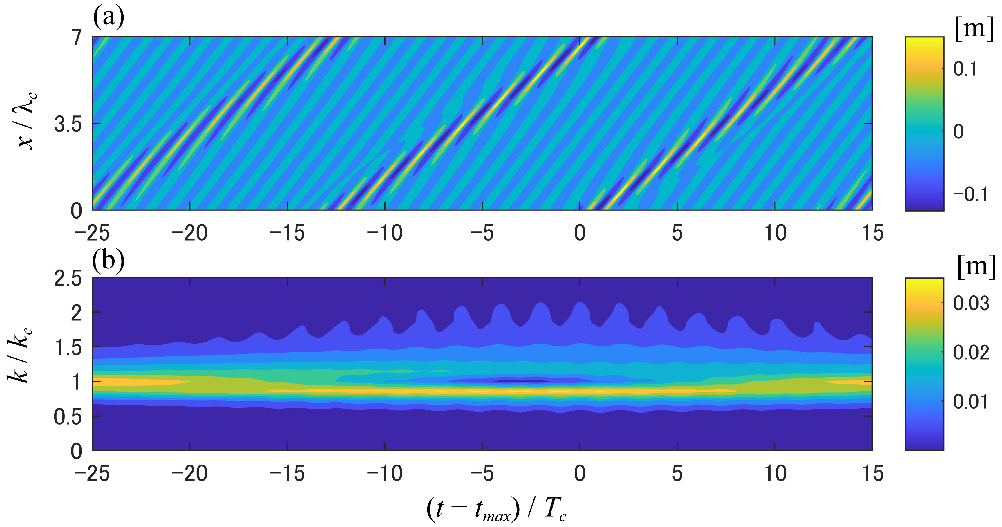
4.2. Phase Convergence during Nonlinear Evolution of a Modulated Wave Train

In Section 4.1, the potential maximum crest height of the modulated wave train was found to increase as the initial wave steepness increased. However, this result does not necessarily indicate an increase in the maximum crest height. Convergence of the phases of all the wave components [31] is necessary to achieve a crest height ζ c r close to its potential maximum A s . In a framework of linear wave superpositions, phase convergence is key to generating focusing waves [31,46]. Slunyaev and Shrira [25] showed that the phases of all the spectral components are nearly coincident in the AB solution. Therefore, in this section, the degree of phase convergence at the location and instant of the maximum crest height is investigated beyond the cubic NLSE regime using the HOSM output.
x m a x is defined as the location of the maximum crest height at each time t . Thus, the maximum crest height at time t is
ζ c r   =   ζ x m a x , t   =   j Re α k j         with       α k j     ζ ^ k j , t exp i k j x m a x .
The modulus and argument of α j express the Fourier amplitude and phase of the component waves at x   =   x m a x at time t , respectively. The phase φ [ arg α ] is defined such that it becomes 0 when the crest of each wave component is at x   =   x m a x .
Figure 12 presents an example of the amplitude and phase of the component waves at t   =   t m a x for a 0 k c   =   0.105 . As observed in the phase spectrum (Figure 12b), most spectral components except the carrier wave at k / k c   =   1 are in phase at 0, especially free-wave components. This feature of phase convergence corresponds to the AB solution with a slight discrepancy. At the modulation peak, all of the AB free-wave components are in phase except for the carrier wave, which is in counter-phase with other components [25]. In this HOSM simulation, the carrier wave is out of phase with sideband waves but not counter-phase.
It is also observed that the phases of some components with lower and higher wavenumbers ( k / k c   <   0.5 and k / k c   >   4 ) are not necessarily 0. Second-order wave theory (Appendix B) explains that the subharmonic bound waves at low wavenumbers are in counter-phase with free waves. In addition, the out-of-phase components at high wavenumbers ( k / k c   >   4 ) consist of free waves, and their energies are very low compared with those of bound waves at the same wavenumbers. Therefore, the contribution of such out-of-phase components at k / k c   >   4 to the crest height is considered almost negligible.
To quantify the degree of phase convergence, the parameter D , expressing the mean of cos φ k j weighted by the Fourier amplitude α k j , is introduced:
D   =   j α k j cos φ k j j α k j   =   j Re α k j j α k j   =   ζ c r A s .
The definition of α is given in Equation (10). As indicated in Equation (11), the parameter D can also be regarded as the ratio of the crest height ζ c r to its potential maximum A s . Figure 13 presents the temporal evolution of D for the modulated wave train with a 0 k c   =   0.105 . Similarly to the evolutions of Δ K and A s , D gradually increases when t   <   t m a x , almost reaches 1 at approximately t   =   t m a x , and starts to decrease afterward ( t   >   t m a x ). This temporal evolution of D confirms almost perfect phase convergence ( D     1 ) near t   =   t m a x . It is interesting to note that the times of the maximum D (indicated with a triangle in Figure 13) and t   =   t m a x do not coincide precisely. Unlike A s , which reaches its maximum a few wave periods after t   =   t m a x (Section 4.1), D reaches its maximum a few wave periods ahead of t   =   t m a x . This time difference will also be discussed in Section 4.3.
To investigate the degree of phase convergence at t   =   t m a x , D at t   =   t m a x for all cases with a 0 k c from 0.08 to 0.115 is presented in Figure 14. D is close to 1 for all cases, although D decreases slightly with increasing a 0 k c . In other words, the phases of all the components nearly coincide at t   =   t m a x , and result in a crest height exceeding 95% of its potential maximum A s for all cases. This result confirms that the near coincidence of the phases of all the spectral components observed in linear focusing waves [31,46] and the free-wave AB solution [25] holds well beyond the NLSE regime. We can also conclude that the phase convergence combined with the free-wave spectral broadening and consequent bound-wave production at high wavenumbers discussed in Section 4.1 is crucial for crest enhancement of modulated wave trains.

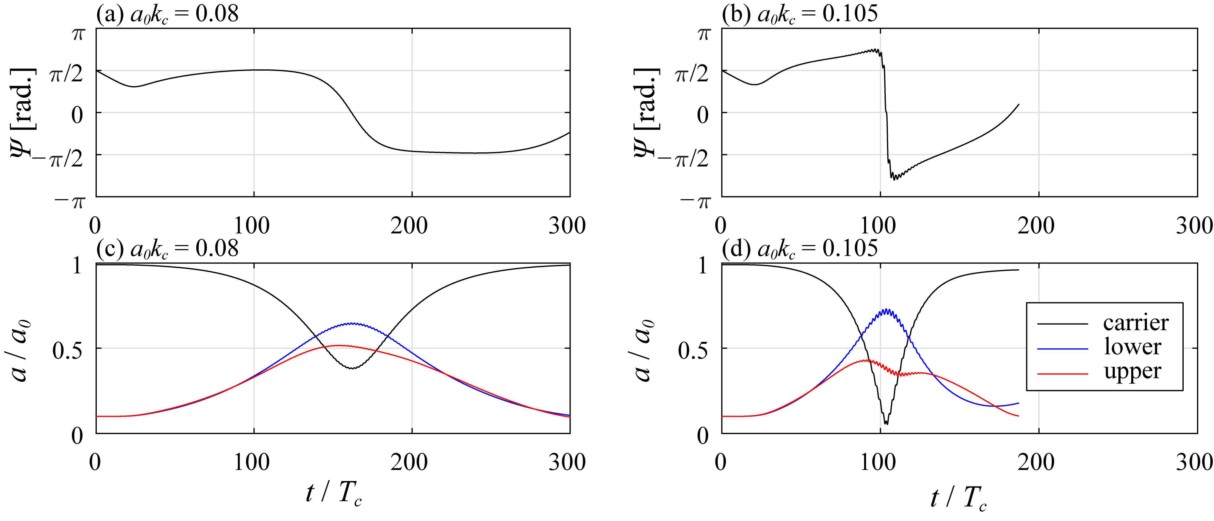
4.3. Temporal Evolution of Phase Relation among the Carrier and Sideband Waves

In Section 4.2, D was found to decrease slightly as a 0 k c increased (Figure 14). This imperfect phase convergence can be attributed to the deviation of the carrier phase from 0 at t   =   t m a x , which is observed in Figure 12b. In this section, this imperfect phase convergence is interpreted in terms of the temporal variation in the phase relation among the carrier, lower-sideband, and upper-sideband waves in the vicinity of t   =   t m a x . The time sequence of the maximum D , maximum ζ c r (corresponding to t   =   t m a x ), and maximum A s is also discussed.
During the nonlinear evolution of modulated wave trains, the carrier wave is phase-locked with the sideband waves. In the initial stage of nonlinear evolution, the phases of the carrier and two sideband components need to satisfy the following relation such that the sideband waves grow exponentially [47,48,49]:
Ψ     2 φ c     φ +     φ   =   c o n s t .   ,
where φ c ,   φ + ,   and φ denote the phases of the carrier, upper-sideband, and lower-sideband waves, respectively. This phase-locked state with Ψ   =   c o n s t . persists on the time scale of O a 0 k c     2 T c until the sideband amplitudes become 20–30% of a 0 , although Ψ   =   c o n s t . is analytically derived assuming that the sideband amplitudes are infinitesimally small compared with the carrier amplitude [47,48,49]. Here, this study focuses on the behavior of Ψ in the vicinity of the modulation peak.
The long-term behavior of Ψ for the modulated wave train is first investigated. Figure 15 presents the temporal evolution of Ψ together with the amplitude evolutions of the carrier, lower sideband, and upper sideband of modulated wave trains with a 0 k c   =   0.08 and 0.105 as examples. Almost a full recurrence cycle is observed for both a 0 k c   =   0.08 and 0.105, although the recurrence period is much shorter for a 0 k c   =   0.105 than for a 0 k c   =   0.08 . Contrary to the theoretical prediction (Equation (12)), Ψ varies in time at the initial stage for both cases. This initial behavior is due to the nonlinear wave initialization of the HOSM simulation explained in Section 2.1. For a 0 k c   =   0.08 , Ψ remains constant at approximately π / 2 after the end of the nonlinear wave initialization and then changes rapidly to π / 2 near the modulation peak (at approximately t / T c   =   162 ). For a 0 k c   =   0.105 , Ψ varies slowly after the end of the nonlinear-wave initialization and, as is the case with a 0 k c   =   0.08 , changes rapidly near the modulation peak (at approximately t / T c   =   104 ). However, its rate of change near the modulation peak is much faster than for a 0 k c   =   0.08 . The time when Ψ = 0 almost corresponds to that when the carrier amplitude reaches its minimum and when the lower-sideband amplitude reaches its maximum for both cases, and when the upper-sideband amplitude reaches its maximum only for a 0   =   0.08 . The constant Ψ at π / 2 just after the nonlinear-wave initialization with a 0 k c   =   0.08 indicates that δ k / k c   =   1 / 7 is the most unstable modulated wavenumber. This gives the highest initial growth rate of the sidebands for an initial wave steepness of 0.08 [48]. In addition, the slow variation in Ψ just after the nonlinear-wave initialization for a 0 k c   =   0.105 implies that the sidebands have imperfect exponential growth due to the nonlinear interaction with wave components other than the initial three waves.
Considering φ and φ + are almost 0 at t   =   t m a x (Figure 12), φ c needs to be 0 for perfect phase convergence. Consequently, Ψ also needs to be 0 at t   =   t m a x . To investigate Ψ at t   =   t m a x , the temporal evolutions of Ψ for the modulated wave trains with a 0 k c   =   0.08 and 0.105 at approximately t   =   t m a x are presented in Figure 16. At t   =   t m a x , Ψ is close to 0 ( Ψ   =     0.078 π ) for a 0 k c   =   0.08 and far from 0 ( Ψ = 0.68 π ) for a 0 k c   =   0.105 . The value of Ψ at t   =   t m a x is related to the difference in time between Ψ   =   0 and t   =   t m a x . In both cases, the time at which Ψ   =   0 is not coincident with t   =   t m a x . Ψ becomes 0 approximately three wave periods ( 3 T c ) ahead of t   =   t m a x . In addition, the variational speed of Ψ ( d Ψ / d t ) is significantly different between the two cases, as already indicated in Figure 15a,b. The variational speed with a 0 k c   =   0.08 is much slower than for a 0 k c   =   0.105 . Therefore, owing to the fast variation in Ψ and the time lag between Ψ   =   0 and t   =   t m a x , Ψ at t   =   t m a x becomes far from 0 with a 0 k c   =   0.105 .
From the observation above, we conjecture that Ψ becomes farther from 0 at t   =   t m a x as a 0 k c increases because of the faster temporal variation in Ψ . To demonstrate this conjecture, Ψ , together with its component phases ( φ c ,   φ , and φ + ), is plotted against a 0 k c at t   =   t m a x in Figure 17. As conjectured, Ψ . at t   =   t m a x becomes farther from 0 as a 0 k c increases. Meanwhile, φ and φ + are confirmed to be close to 0 regardless of a 0 k c . Accordingly, φ c becomes farther from zero at t   =   t m a x as a 0 k c increases. Thus, the slight decrease in degree of phase convergence D at t   =   t m a x with increasing a 0 k c (Figure 14) can be attributed to φ c being out of phase with φ and φ + . The evolution of the phase relation among the carrier, lower-sideband, and upper-sideband waves is found to affect the degree of phase convergence at t   =   t m a x .
Lastly, the sequence of times at which t   =   t m a x , Ψ   =   0 , and D and A s reach their maxima is discussed. These are plotted against a 0 k c in Figure 18. The following features, which have been found so far for modulated wave trains with specific a 0 k c values, seem to be robust regardless of a 0 k c : A s reaches its maximum about 3 T c to 5 T c after t   =   t m a x , D reaches its maximum about 2 T c ahead of t   =   t m a x , and Ψ is 0 approximately 2 T c to 4 T c ahead of t   =   t m a x . The close times of maximum D and Ψ   =   0 indicate that D reaches its maximum when the carrier, lower-sideband, and upper-sideband waves are in phase because the contribution of these three components to D is dominant. Figure 18 also reveals that the time of maximum A s necessarily lags behind that of maximum D regardless of a 0 k c . The degree of phase convergence D and the potential maximum crest height D are the two most significant factors determining the actual maximum crest height. Consequently, we can surmise that the crest height reaches its maximum ( t   =   t m a x ) midway between the times of maximum D and maximum A s .

5. Conclusions

The most notable finding of this study is that the phases of all the spectral wave components of the nonlinearly evolving modulated wave trains coincided at the peak of the modulation. This phase convergence process contributes to the crest enhancement of modulated wave trains beyond the AB solution of the cubic NLSE. However, this phase convergence is a nonlinear process where the phases change in time and is not a linear dispersive focusing where the initial phases are stationary. This was unraveled by numerical examinations based on HOSM up to the fifth order in a non-breaking potential-flow regime. HOSM allowed investigation of nonlinearity and spectral bandwidth beyond the NLSE regime. Scrutinizing HOSM outputs also revealed two other critical physical processes of such crest enhancement: spectral broadening and bound-wave production. The free wave spectra of modulated wave trains in the HOSM simulation broaden beyond the AB solution because of the unrestricted spectral bandwidth in the HOSM simulation. The free-wave spectral broadening energizes the bound-wave production at high wavenumbers. The bound wave components can contribute more than a quarter of the maximum crest height at an initial wave steepness of 0.115.
The finding regarding the phase convergence implies that distinguishing from a single point measurement if an observed rogue wave was generated due to linear focusing or modulational instability may not be possible. Contrary to a recent study by Gemmrich and Cicon [50] that explained the observed rogue wave by the superposition of linear waves with fourth-order Stokes wave correction, our findings suggests paying much closer attention to the evolutionary process leading to rogue wave formation.
Finally, this study has elucidated the significance of the strong nonlinearity in the evolution of the modulated wave train. When wave-breaking occurs, the maximum crest in the tank falls below the HOSM simulation. However, with a sufficiently large initial wave steepness but without wave breaking, the highest crest in the tank exceeds the HOSM simulation due to a strong nonlinearity. The first finding is not surprising, but the second finding highlights the significance of the strong nonlinearity and warrants further study.

Author Contributions

Conceptualization, H.H. and T.W.; methodology, H.H. and H.S.; software, H.H. and T.W.; validation, H.H.; formal analysis, H.H.; investigation, H.H., H.S. and T.W.; resources, H.H. and H.S.; data curation, H.H.; writing—original draft preparation, H.H.; writing—review and editing, H.H. and T.W.; visualization, H.H.; supervision, T.W.; project administration, H.H.; funding acquisition, H.H. and T.W. All authors have read and agreed to the published version of the manuscript.

Funding

This research was funded by JSPS KAKENHI grant numbers JP 16H02429, JP21H01538, and JP22H01136.

Institutional Review Board Statement

Not applicable.

Informed Consent Statement

Not applicable.

Data Availability Statement

The data are available upon request.

Acknowledgments

We thank Katsuji Tanizawa for useful discussions. Mark Kurban from Edanz (https://jp.edanz.com/ac (accessed on 6 August 2022)), Lai Roxanne and Paul Consalvi from the University of Tokyo edited a draft of this paper.

Conflicts of Interest

The authors declare no conflict of interest.

Appendix A. Akhmediev Breather Solution

The Akhmediev breather solution of the NLSE in deep water reads [20]
B x , t   =   a 0 exp     i 2 ϵ 2 ω c t ρ cosh Ω t     i γ sinh Ω t cosh Ω t     1     ρ 2 / 2 cos k c x     c g c t / N k     1
with
ϵ   =   a 0 k c ,   c g c   =   1 2 ω c k c ,   ρ   =   1 2 ϵ N k ,   γ   =   2 2 ϵ N k 1     1     1 2 2 ϵ N k 2 , Ω   =   1 2 γ ϵ 2 ω c ,   N k   =   k c δ k   ,
where B x , t is the complex amplitude of the surface elevation ζ x , t . The term δ ^ defined in Equation (4) corresponds to the inverse of ϵ N k :
δ ^   =   1 2 ϵ N k .
Within the framework of the deep-water NLSE, ζ x , t can be expressed as follows considering the nonlinearity up to the second order [51,52]:
ζ x , t ζ f + b x , t   =   ζ f x , t   +   ζ b x , t
with
ζ f x , t   =   R e B exp i k c x     ω c t , ζ b x , t   =   R e 1 2 k c B 2 exp 2 i k c x     ω t ,  
where ζ f x , t and ζ b x , t represent the free wave and second-order bound wave, respectively.
The maximum amplitude, which corresponds to the maximum crest height, of the free wave is attained at x , t   =   0 , 0 and reads [18,19,20,25]
max ζ f a 0   =   1   +   2 1     1 2 δ ^ 2 .
From Equations (A4)–(A6), the maximum crest height considering the contribution of the second-order bound wave can be expressed as
max ζ f   +   b a 0   =   max ζ f a 0 1   +   1 2 k c max ζ f .

Appendix B. Phase of Second-Order Superharmonic and Subharmonic Waves

In this section, the relation between the phases of the free and second-order bound waves is investigated. The second-order bound waves produced by a pair of free waves propagating in the positive x direction are addressed. The free-surface elevation x consisting of a pair of free waves with wavenumbers k 1 and k 2 is expressed as
ζ 1 x , t   =   j = 1 2 ζ ^ j cos θ j
with
θ j   =   k j x     ω j t + γ j ,
where j   =   1 ,   2 and γ denote the indexes of the free waves and the initial phase, respectively. Deep water and k 1     k 2     0 are assumed. The second-order bound waves ζ 2 produced by the pair of free waves (Equations (A8) and (A9)) are expressed as [53]
ζ 2 x , t   =   j = 1 2 ζ ^ j 2 k j 2 cos 2 θ j   +   ζ ^ 1 ζ ^ 2 k 1   +   k 2 2 cos θ 1 + θ 2   +   ζ ^ 1 ζ ^ 2     k 1     k 2 2 cos θ 1     θ 2 .
The first two terms represent superharmonics, and the last term represents subharmonics.
Here, the free waves are assumed to be in phase at a specific time ( t   =   t 0 ) and location ( x   =   x 0 ); that is, θ 1   =   θ 2   =   0 . Then, the free and the second-order bound-wave solution reads
ζ 1 x 0 , t 0   =   j = 1 2 ζ ^ j , ζ 2 x 0 , t 0   =   j = 1 2 ζ ^ j 2 k j 2   +   ζ ^ 1 ζ ^ 2 k 1   +   k 2 2   +   ζ ^ 1 ζ ^ 2     k 1     k 2 2 .
Only the second-order subharmonic component is negative, although the free-wave and second-order superharmonic components are positive. Therefore, when all the free-wave components are in phase, the second-order superharmonics are in phase, and subharmonics are in counter-phase with the free waves.

References

  1. Welch, S.; Levi, C.; Fontaine, E.; Tulin, M.P. Experimental loads on a flexibly mounted vertical cylinder in breaking wave groups. In Proceedings of the Eighth International Offshore and Polar Engineering Conference, Montreal, QC, Canada, 24–29 May 1998; OnePetro: Richardson, TX, USA, 1998. [Google Scholar]
  2. Onorato, M.; Proment, D.; Clauss, G.; Klein, M. Rogue waves: From nonlinear Schrödinger breather solutions to sea-keeping test. PLoS ONE 2013, 8, e54629. [Google Scholar] [CrossRef]
  3. Klein, M.; Clauss, G.F.; Rajendran, S.; Soares, C.G.; Onorato, M. Peregrine breathers as design waves for wave-structure interaction. Ocean. Eng. 2016, 128, 199–212. [Google Scholar] [CrossRef]
  4. Houtani, H.; Waseda, T.; Tanizawa, K.; Sawada, H. Temporal variation of modulated-wave-train geometries and their influence on vertical bending moments of a container ship. Appl. Ocean. Res. 2019, 86, 128–140. [Google Scholar] [CrossRef]
  5. Shahroozi, Z.; Göteman, M.; Engström, J. Experimental investigation of a point-absorber wave energy converter response in different wave-type representations of extreme sea states. Ocean. Eng. 2022, 248, 110693. [Google Scholar] [CrossRef]
  6. Bitner-Gregersen, E.M.; Toffoli, A. On the probability of occurrence of rogue waves. Nat. Hazards Earth Syst. Sci. 2012, 12, 751–762. [Google Scholar] [CrossRef]
  7. Bitner-Gregersen, E.M.; Gramstad, O. Rogue waves impact on ships and offshore structures. In Det Norske Veritas Germanischer Lloyd Strategic Research and Innovation Position Paper; DNV: Bærum, Norway, 2015. [Google Scholar]
  8. Forristall, G.Z. Maximum wave heights over an area and the air gap problem, OMAE2006-92022 paper. In Proceedings of the ASME 25th International Conference on Ocean Offshore, and Arctic Engineering, Hamburg, Germany, 4–9 June 2006. [Google Scholar]
  9. Magnusson, A.K.; Donelan, M.A. The Andrea wave characteristics of a measured North Sea rogue wave. J. Offshore Mech. Arct. Eng. 2013, 135, 31108. [Google Scholar] [CrossRef]
  10. Janssen, P.A. Nonlinear four-wave interactions and freak waves. J. Phys. Oceanogr. 2003, 33, 863–884. [Google Scholar] [CrossRef]
  11. Onorato, M.; Waseda, T.; Toffoli, A.; Cavaleri, L.; Gramstad, O.; Janssen, P.A.E.M.; Kinoshita, T.; Monbaliu, J.; Mori, N.; Osborne, A.R.; et al. Statistical properties of directional ocean waves: The role of the modulational instability in the formation of extreme events. Phys. Rev. Lett. 2009, 102, 114502. [Google Scholar] [CrossRef]
  12. Waseda, T.; Kinoshita, T.; Tamura, H. Evolution of a random directional wave and freak wave occurrence. J. Phys. Oceanogr. 2009, 39, 621–639. [Google Scholar] [CrossRef]
  13. Benjamin, T.B.; Feir, J.E. The disintegration of wave trains on deep water Part 1. Theory. J. Fluid Mech. 1967, 27, 417–430. [Google Scholar] [CrossRef]
  14. Benjamin, T.B. Instability of periodic wavetrains in nonlinear dispersive systems. Proc. R. Soc. Lond. Ser. A Math. Phys. Sci. 1967, 299, 59–76. [Google Scholar]
  15. Tulin, M.P.; Waseda, T. Laboratory observations of wave group evolution, including breaking effects. J. Fluid Mech. 1999, 378, 197–232. [Google Scholar] [CrossRef]
  16. Stiassnie, M.; Kroszynski, U.I. Long-time evolution of an unstable water-wave train. J. Fluid Mech. 1982, 116, 207–225. [Google Scholar] [CrossRef]
  17. Akhmediev, N.N.; Eleonskii, V.M.; Kulagin, N.E. Exact first-order solutions of the nonlinear Schrödinger equation. Theor. Math. Phys. 1987, 72, 809–818. [Google Scholar] [CrossRef]
  18. Onorato, M.; Osborne, A.R.; Serio, M. Nonlinear Dynamics of Rogue Waves. In Proceedings of the International Workshop on Wave Hindcasting and Forecasting, Monterey, CA, USA, 6–10 November 2000; pp. 470–479. [Google Scholar]
  19. Onorato, M.; Osborne, A.R.; Serio, M.; Damiani, T. Occurrence of freak waves from envelope equations in random ocean wave simulations. In Proceedings of the Rogue Wave 2000, Brest, France, 29–30 November 2000; pp. 181–191. [Google Scholar]
  20. Onorato, M.; Residori, S.; Bortolozzo, U.; Montina, A.; Arecchi, F.T. Rogue waves and their generating mechanisms in different physical contexts. Phys. Rep. 2013, 528, 47–89. [Google Scholar] [CrossRef]
  21. Mori, N.; Janssen, P.A. On kurtosis and occurrence probability of freak waves. J. Phys. Oceanogr. 2006, 36, 1471–1483. [Google Scholar] [CrossRef]
  22. Su, M.Y.; Green, A.W. Coupled two-and three-dimensional instabilities of surface gravity waves. Phys. Fluids 1984, 27, 2595–2597. [Google Scholar] [CrossRef]
  23. Waseda, T. Experimental investigation and applications of the modulational wave train. In Proceedings of the Workshop on Rogue Waves, Honolulu, HI, USA, 25–28 January 2005; pp. 12–15. [Google Scholar]
  24. Tanaka, M. Maximum amplitude of modulated wavetrain. Wave Motion 1990, 12, 559–568. [Google Scholar] [CrossRef]
  25. Slunyaev, A.V.; Shrira, V.I. On the highest non-breaking wave in a group: Fully nonlinear water wave breathers versus weakly nonlinear theory. J. Fluid Mech. 2013, 735, 203–248. [Google Scholar] [CrossRef]
  26. Zakharov, V.E. Stability of periodic waves of finite amplitude on the surface of a deep fluid. J. Appl. Mech. Tech. Phys. 1968, 9, 190–194. [Google Scholar] [CrossRef]
  27. Dold, J.W.; Peregrine, D.H. An efficient boundary-integral method for steep unsteady water waves. Numer. Methods Fluid Dyn. II 1986, 671, 679. [Google Scholar]
  28. Dysthe, K.B. Note on a modification to the nonlinear Schrödinger equation for application to deep water waves. Proc. R. Soc. Lond. A Math. Phys. Sci. 1979, 369, 105–114. [Google Scholar]
  29. Chabchoub, A.; Kibler, B.; Dudley, J.M.; Akhmediev, N. Hydrodynamics of periodic breathers. Philos. Trans. R. Soc. A Math. Phys. Eng. Sci. 2014, 372, 20140005. [Google Scholar] [CrossRef] [PubMed]
  30. Zakharov, V.E.; Dyachenko, A.I.; Vasilyev, O.A. New method for numerical simulation of a nonstationary potential flow of incompressible fluid with a free surface. Eur. J. Mech. B Fluids 2002, 21, 283–291. [Google Scholar] [CrossRef]
  31. Chaplin, J.R. On frequency-focusing unidirectional waves. Int. J. Offshore Polar Eng. 1996, 6, 131–137. [Google Scholar]
  32. West, B.J.; Brueckner, K.A.; Janda, R.S.; Milder, D.M.; Milton, R.L. A new numerical method for surface hydrodynamics. J. Geophys. Res. Ocean. 1987, 92, 11803–11824. [Google Scholar] [CrossRef]
  33. Dommermuth, D.G.; Yue, D.K. A high-order spectral method for the study of nonlinear gravity waves. J. Fluid Mech. 1987, 184, 267–288. [Google Scholar] [CrossRef]
  34. Stokes, G.G. On the theory of oscillatory waves. Trans. Camb. Philos. Soc. 1847, 8, 441–455. [Google Scholar]
  35. Houtani, H.; Waseda, T.; Tanizawa, K. Experimental and numerical investigations of temporally and spatially periodic modulated wave trains. Phys. Fluids 2018, 30, 34101. [Google Scholar] [CrossRef]
  36. Houtani, H.; Waseda, T.; Fujimoto, W.; Kiyomatsu, K.; Tanizawa, K. Generation of a spatially periodic directional wave field in a rectangular wave basin based on higher-order spectral simulation. Ocean. Eng. 2018, 169, 428–441. [Google Scholar] [CrossRef]
  37. Kirezci, C.; Babanin, A.V.; Chalikov, D.V. Modelling rogue waves in 1D wave trains with the JONSWAP spectrum, by means of the High Order Spectral Method and a fully nonlinear numerical model. Ocean. Eng. 2021, 231, 108715. [Google Scholar] [CrossRef]
  38. Tanaka, M. A method of studying nonlinear random field of surface gravity waves by direct numerical simulation. Fluid Dyn. Res. 2001, 28, 41. [Google Scholar] [CrossRef]
  39. Tian, Z.; Perlin, M.; Choi, W. Evaluation of a deep-water wave breaking criterion. Phys. Fluids 2008, 20, 66604. [Google Scholar] [CrossRef]
  40. Dommermuth, D. The initialization of nonlinear waves using an adjustment scheme. Wave Motion 2000, 32, 307–317. [Google Scholar] [CrossRef]
  41. Houtani, H.; Waseda, T.; Tanizawa, K. Measurement of spatial wave profiles and particle velocities on a wave surface by stereo imaging–validation with unidirectional regular waves. J. Jpn. Soc. Nav. Archit. Ocean. Eng. 2017, 25, 93–102. (In Japanese) [Google Scholar]
  42. Houtani, H.; Waseda, T.; Fujimoto, W.; Kiyomatsu, K.; Tanizawa, K. Freak wave generation in a wave basin with HOSM-WG method. In Proceedings of the International Conference on Offshore Mechanics and Arctic Engineering, St. John’s, NL, Canada, 31 May–5 June 2015; American Society of Mechanical Engineers: New York, NY, USA, 2015; Volume 56550, p. V007T06A085. [Google Scholar]
  43. Thyagaraja, A. Recurrent motions in certain continuum dynamical systems. Phys. Fluids 1979, 22, 2093–2096. [Google Scholar] [CrossRef]
  44. Martin, D.U.; Yuen, H.C. Spreading of energy in solutions of the nonlinear Schrödinger equation. Phys. Fluids 1980, 23, 1269–1271. [Google Scholar] [CrossRef]
  45. Gibson, R.S.; Swan, C. The evolution of large ocean waves: The role of local and rapid spectral changes. Proc. R. Soc. A Math. Phys. Eng. Sci. 2007, 463, 21–48. [Google Scholar] [CrossRef]
  46. Rapp, R.J.; Melville, W.K. Laboratory measurements of deep-water breaking waves. Philos. Trans. R. Soc. Lond. Ser. A Math. Phys. Sci. 1990, 331, 735–800. [Google Scholar]
  47. Waseda, T. Laboratory Study of Wind-and Mechanically-Generated Water Waves. Ph.D. Thesis, University of California, Santa Barbara, CA, USA, 1997. [Google Scholar]
  48. Waseda, T.; Tulin, M.P. Experimental study of the stability of deep-water wave trains including wind effects. J. Fluid Mech. 1999, 401, 55–84. [Google Scholar] [CrossRef]
  49. Liu, S.; Waseda, T.; Zhang, X. Phase Locking Phenomenon in the Modulational Instability of Surface Gravity Waves. In Proceedings of the 36th International Workshop on Water Waves and Floating Bodies (IWWWFB), Seoul, Korea, 25–28 April 2021; pp. 117–120. [Google Scholar]
  50. Gemmrich, J.; Cicon, L. Generation mechanism and prediction of an observed extreme rogue wave. Sci. Rep. 2022, 12, 1718. [Google Scholar] [CrossRef] [PubMed]
  51. Slunyaev, A.V. A high-order nonlinear envelope equation for gravity waves in finite-depth water. J. Exp. Theor. Phys. 2005, 101, 926–941. [Google Scholar] [CrossRef]
  52. Chabchoub, A.; Hoffmann, N.; Onorato, M.; Akhmediev, N. Super rogue waves: Observation of a higher-order breather in water waves. Phys. Rev. X 2012, 2, 11015. [Google Scholar] [CrossRef]
  53. Dalzell, J.F. A note on finite depth second-order wave-wave interactions. Appl. Ocean. Res. 1999, 21, 105–111. [Google Scholar] [CrossRef]
Figure 1. (a) Time series of wave elevation of the modulated wave train with a 0 k c   =   0.08 simulated with the HOSM. (b) Enlarged view of (a) around the time of the maximum crest height ( t   =   t m a x ), which is compared with the corresponding wave-elevation at x   =   12 m measured in the wave tank.
Fluids 07 00275 g001
Figure 2. Schematic of the stereo camera set up in the wave tank (WT).
Fluids 07 00275 g002
Figure 3. Variation in maximum crest height with the initial wave steepness. f and b indicate the free and second-order bound waves, respectively.
Fluids 07 00275 g003
Figure 4. Comparison of the Fourier amplitudes of the modulated wave trains in the frequency domain among the experiment, HOSM simulation, and AB solution for (a) a 0 k c   =   0.100 (non-breaking) and (b) a 0 k c   =   0.1025 (slight breaking).
Fluids 07 00275 g004
Figure 5. Temporal evolution of the modulated wave train with a 0 k c   =   0.105 near the time of the maximum crest height ( t   =   t m a x ) in the HOSM simulation. (a) Wave elevation ζ x , t ; (b) amplitude spectrum ζ ^ k , t .
Fluids 07 00275 g005
Figure 6. Temporal evolution of the mean wavenumber difference Δ K / δ k of the modulated wave train with a 0 k c   =   0.105 at approximately the time of the maximum crest height ( t   =   t m a x ) in the HOSM simulation. The dashed line represents the initial value.
Fluids 07 00275 g006
Figure 7. Relation between the initial wave steepness a 0 k c and mean wavenumber difference Δ K / δ k at t   =   t m a x for the modulated wave train. The dashed line represents the initial value.
Fluids 07 00275 g007
Figure 8. Comparison of the Fourier amplitudes of the modulated wave trains with a 0 k c   =   0.105 in the wavenumber domain at the time of the maximum crest height in the HOSM simulation and AB solution. Note that the bound-wave spectrum of the HOSM simulation breaks around k / k c because its spectral energy is removed owing to the ideal filter separating free and bound waves.
Fluids 07 00275 g008
Figure 9. Relation between the initial wave steepness a 0 k c and mean wavenumber difference Δ K / δ k at t   =   t m a x for the modulated wave train. (a) Free wave; (b) bound wave.
Fluids 07 00275 g009
Figure 10. Temporal evolution of the amplitude sum A s of the modulated wave train with a 0 k c   =   0.105 at approximately the time of the maximum crest height ( t   =   t m a x ) in the HOSM simulation. The dashed line represents the initial value, and the triangle indicates the maximum value.
Fluids 07 00275 g010
Figure 11. (a) Relation between the spectral broadening Δ K / δ k and amplitude sum A s / a 0 of the modulated wave train. (b) Relation between the free-wave spectral broadening Δ K f / δ k and amplitude sum A s / a 0 of the modulated wave train for the total, free-wave, and bound-wave components.
Fluids 07 00275 g011
Figure 12. (a) Amplitude and (b) phase of the component waves of the modulated wave train with a 0 k c   =   0.105 at the location and time of the maximum crest height.
Fluids 07 00275 g012
Figure 13. Temporal evolution of the phase convergence D of the modulated wave train with a 0 k c   =   0.105 at approximately the time of the maximum crest height ( t   =   t m a x ) in the HOSM simulation. The triangle indicates the maximum value.
Fluids 07 00275 g013
Figure 14. Relation between the initial wave steepness and degree of phase convergence at the time of the maximum crest height, obtained from the HOSM simulation.
Fluids 07 00275 g014
Figure 15. Long-term temporal evolutions of (a,b) Ψ and (c,d) the amplitudes of the carrier, lower-sideband, and upper-sideband components of the modulated wave train with a 0 k c   =   0.08 (a,c) and 0.105 (b,d).
Fluids 07 00275 g015
Figure 16. Temporal evolution of Ψ for the modulated wave train at approximately the time of the maximum crest height ( t   =   t m a x ) for (a) a 0 k c   =   0.08 and (b) a 0 k c   =   0.105 . Circles indicate the times at which Ψ   =   0 .
Fluids 07 00275 g016
Figure 17. Variations of Ψ . and the carrier, lower-sideband, and upper-sideband phases at the time of maximum crest height against initial wave steepness a 0 k c .
Fluids 07 00275 g017
Figure 18. Variations in times of maximum crest height ( ζ c r .), Ψ   =   0 , maximum degree of phase convergence ( D ), and maximum amplitude sum ( A s ) against initial wave steepness a 0 k c .
Fluids 07 00275 g018
Table 1. Parameters defining the initial profiles of the modulated wave trains simulated with the HOSM. a 0 = a c 2   +   a + 2   +   a 2 1 / 2 denotes the initial amplitude of the Stokes wave.
ParametersValues
wavelength   λ c = 2 π / k c 3 m
perturbation   wavenumber   δ k / k c 1/7
sideband   wave   amplitudes   a ± / a 0 0.1
sideband   wave   phases   φ ± π / 4
wave   steepness   a 0 k c 0.08–0.115
δ ^ 0.62–0.89
Publisher’s Note: MDPI stays neutral with regard to jurisdictional claims in published maps and institutional affiliations.

