Article

A 3D CFD-Based Workflow for Analyses of a Wide Range of Flow and Heat Transfer Conditions in Air Gaps of Electric Machines

Faculty of Mechanical Engineering, University of Ljubljana, Aškerčeva 6, SI-1000 Ljubljana, Slovenia
*
Authors to whom correspondence should be addressed.
Fluids 2022, 7(8), 273; https://doi.org/10.3390/fluids7080273
Submission received: 12 July 2022 / Revised: 4 August 2022 / Accepted: 6 August 2022 / Published: 10 August 2022

Abstract

:
Increasing power densities of electric machines in e-vehicles in addition to the resulting quest for enhanced cooling concepts are bringing forward the importance of defining adequate heat transfer correlations in air gaps. This is a highly challenging topic, as there exist no generally applicable flow and heat transfer phenomena descriptions for air gaps due to their highly variable geometrical properties and operating conditions. As an answer to this challenge, this paper presents a workflow that defines an adequate 3D CFD model for an arbitrary air-gap design that includes its system-dependent boundary conditions. The workflow is built on the recognition of underlying air-gap flow phenomena, which are used to steer the subsequent design of the 3D CFD model in a systematic step-by-step manner. Consequently, the complexity of the 3D CFD model gradually increases to the point where it provides an adequate flow and heat transfer description. Validation of the workflow is presented for a wide range of air-gap designs and flow conditions. It is demonstrated that the 3D CFD models obtained with the workflow match the experimentally obtained data from various flow cases that have been documented in the literature. Considerable optimization of computational costs, offering potentially an order-of-magnitude reduction in computational time, is achieved as a result of computational domain span optimization and transient simulations being applied only when required. The validation confirms that this workflow facilitates construction of valid 3D CFD models without the prior knowledge of flow and heat transfer phenomena in a specific air gap. This workflow thus provides a reliable and computationally efficient tool for valorization of convective heat transfer, and opens up prospects for time- and cost-efficient optimizations of electric machines’ cooling system designs.

1. Introduction

Manufacturers are constantly trying to reduce the mass of electrified vehicles, particularly of their powertrains, while simultaneously increasing their efficiency and reducing their production costs. An objective of this process is to achieve increased power densities of propulsion components, such as electric machines (EM). Higher power densities inherently require efficient cooling for safe and reliable operation. This is especially important for an EM with permanent magnets, as their demagnetization temperatures define operating temperature limits. The temperatures of these magnets are, amongst other impacts, affected by the flow conditions in the air gap, which determine the heat transfer between the rotor and the stator. The ability to define these flow conditions, as well as their heat transfer, is thus necessary in order to predict cooling requirements and capabilities for short-term overloads. Consequently, the conditions in the air gap have an important impact on electromagnetics, which means that they influence the design of the thermal management system, and by this, also the performance and economic aspects.
Defining heat transfer in an air gap or, more generally, annular gap between two concentric cylinders of various surface configurations, is challenging due to the various flow phenomena that can be present. In general, it is possible to distinguish between two main flow types. The most often encountered type features no axial flow, and is referred to as Taylor–Couette (TC) flow, following the pioneering works of Couette [1] and Taylor [2]. Considerably different flow phenomena can be observed if axial flow is present. This flow type is referred to as Taylor–Couette–Poiseuille (TCP) flow. The appearance of both flow types is affected by the presence of smooth or grooved surfaces, and by various aspect ratios of air gaps. The broad variety of geometrical configurations translates the two basic flow types into a large variety of flow phenomena, resulting in highly variable heat transfer phenomena. This has led to numerous experimental and numerical studies. Various air gaps with different imposed conditions were considered, in order to provide to them specific flow and heat transfer characterizations. However, no universal correlations were defined. This is an important challenge regarding the development of Ems [3], and is related to another challenging aspect, which is the lack of a universally applicable approach for defining heat transfer in air gaps. The ability to perform systematic exploration of an EM design space is thus hindered, which makes virtual development more time consuming.
Considering experimental studies, the early research of Kaye and Elgar [4] identified four main flow modes that can appear in air-gap flow. These modes are distinguished by the presence of laminar or turbulent flow, and their combination, along with specific flow structures called Taylor vortices. The main modes as well as their dependencies on imposed axial flow and cylinder rotation velocities are shown in Figure 1, alongside the illustration of the Taylor vortices. These appear in counter-rotating pairs whenever a critical rotational velocity is exceeded, and notably affect the magnitude of convective heat transfer. Their appearance was further studied under various conditions in TCP flow by Gardiner and Sabersky [5]. While Gardiner and Sabersky [5] focused on long gaps, the research of Lee and Minkowicz [6] intentionally focused on short annular gaps, where the importance of yet another flow phenomenon, the entrance region, was recognized. In addition to the presence of an entrance region, the study by Bouafia [7] also focused on the influence of grooved and smooth stator surfaces on heat transfer. It was shown that grooved surfaces improve heat transfer. Further insights into flow and heat transfer phenomena were recently obtained by the introduction of flow visualization. Fénot [8] applied PIV measurements in conjunction with temperature measurements using an IR camera in the entrance region as well as along an annular gap with a grooved rotor. Liu [9] also applied a PIV method to investigate the temperature gradient influence on heat transfer in TC flows. Aubert [10] further combined PIV methods with LDV and temperature measurements in order to obtain a comprehensive description of flow field in a narrow, long and smooth gap. Yet, in spite of applying advanced experimental methods, there are still many areas where air-gap flow and heat transfer are only partially characterized. The recent review paper by Fénot [11] notes that there exists a significant lack of heat transfer correlations for grooved air gaps, which is highly relevant due to their presence in EMs. For instance, the influence of the number of grooves as well as their aspect ratio on the friction factor and heat transfer in air gaps with grooves on the stator were researched only recently by Nouri-Borujerdi in TC [12] and TCP flows [13]. What presents an even larger challenge is that important discrepancies in heat transfer correlations can be observed between experimental works. For instance, Fénot [11] points to the differences in conditions at which Taylor vortices appear in different air gaps. This then leads to differences in correlations for Nusselt numbers, noted also in [14]. These correlations must be given for each gap, acknowledging the imposed conditions in it. These differences between correlations exist among smooth annular gaps, and are even more apparent for grooved gaps. A number of reasons for these differences are provided in the review by Fénot [11]. The most apparent reason is the high variability in air-gap shapes, as there exist considerable differences between the geometrical aspect ratios of air gaps in various studies. Aside from these geometrical differences, there also exist notable differences in imposed thermal conditions on the rotor and stator between various studies. Finally, the air-gap entrance conditions often differ, leading to different flow evolutions in air gaps, and hence also leading to differences in the defined heat transfer correlations. Finally, Bouafia [7] also points to differences in the applied definitions used for dimensionless numbers among different studies, which present yet another cause for the noted discrepancies between heat transfer correlations.
It can be thus concluded that in spite of significant past efforts and achievements, there still exist many areas where flow and heat transfer phenomena in air gaps are not completely characterized, while considerable discrepancies between reported results exist as well. A resolution of these challenges could be achieved through a universally applicable approach for defining air-gap flow and heat transfer phenomena. The great variety in air-gap geometry and operational conditions would make this approach highly challenging and expensive in the case of relying on experimental measurements. On the contrary, the simple adaptability of 3D CFD models in addition to their ability to model various flows present a plausible option to alleviate these constraints. Furthermore, a systematic exploration of an EM design space is in general more practical, with adequate 3D CFD models for various imposed conditions in an EM.
Considering CFD, the literature reveals that different numerical methods can be applied in modelling air-gap flows. Finite volume methods are most often used, and the following review focuses on these. However, other methods have also been applied successfully. The lattice Boltzmann method, applied in TC flow simulations in [15], can be stressed. It is gaining in popularity, and hence becoming increasingly developed, spreading to the fields of fluid–structure interaction simulations [16] and non-Newtonian fluids [17]. The different numerical methods can be coupled with different modelling approaches, in order to study various annular gap flows. In one of the early works, where only laminar flow modelling was applied, Hayase [18] showed that 3D simulations with periodic conditions in the azimuth direction are generally required for TC flow in grooved gaps. Bouafia [19] then performed such simulations to obtain global and local Nusselt numbers in smooth and grooved gaps. However, Sommerer and Lauriat [20] showed that under certain conditions, 2D simulations that consider only radial and azimuthal discretization are sufficient. On the contrary, Hwang and Yang [21] considered the complete domain to capture Taylor vortices of various shapes in laminar TCP flow conditions in a smooth gap. With increases in computational power and in the capabilities of turbulent models, turbulent flow conditions began to be studied, and different modelling approaches were used with them as well. For instance, in Poncet and Haddadi [22], the Reynolds stress model is applied in 2D axisymmetric simulations to describe TC flow development in a narrow smooth gap. In Poncet and da Soghe [23], RANS, LES and DNS flow modelling are used to describe TC flow in a smooth gap with a low aspect ratio. Foundrinier and Poncet [24] applied RANS and LES models in TCP flow simulations, where connections between entrance region length and flow parameters are discussed. Recently, Hamidi and Poncet [3] argued that the k-ω SST model is most practical in describing TCP flow that is subjected to a temperature gradient. Fewer published works are available for grooved annular gaps, yet they are also aimed at modelling flow under different geometries and conditions. For instance, Romanozzi and Howey [25] studied TC flow in an annular gap with a grooved rotor, and periodic boundary conditions in the azimuth and axial directions. Lancial and Torriano in [26], and later in [27], performed simulations of an annular gap with a grooved rotor to describe cases where axial or tangential velocity has a dominant effect on the flow field. In relation to experimental studies in [12,13], Nouri [28] performed RANS simulations to obtain numerical descriptions of flow and heat transfer phenomena in air gaps with various shapes of grooves. The listed papers depict that, similarly with experimental studies, various annular gap geometries with various conditions were a subject of numerical studies. Moreover, similarly with experimental studies, each numerical study considered only specific air-gap shapes and operating conditions. Consequently, these studies do not deal with the question of how to define 3D CFD models for a large variety of flow cases. Initial attempts that approach this challenge can be found in the mentioned studies by Lancial and Torriano [26,27]. However, the model in these studies is set by preliminary TC flow simulations, while the final presented results concern TCP flow conditions. Although valid final numerical results are provided, it is not generally applicable to define a model in this manner, as the differences between TC and TCP flow phenomena may be too large. Thus, there still exists an important knowledge gap in providing guidelines on how to define 3D CFD models for valid EM air-gap flow and heat transfer simulations.
In order to address this knowledge gap, this paper presents a workflow that defines adequate 3D CFD models for an arbitrary air gap with a whole range of operating conditions imposed upon it. Importantly, this workflow does not aim to propose one 3D CFD model. Instead, by recognizing the high variability in flow phenomena in an air gap, it provides an adequate model for each of the observed flow conditions. In this manner, the proposed workflow also provides a more adequate foundation for the systematic exploration of an EM design space. In order to achieve this, it applies a systematic step-by-step approach, in which adequate models for the observed conditions are constructed by accounting for different and, until now, not simultaneously addressed flow aspects. The key to achieving this is found in the definition of the underlying flow characteristics that are presented by flow steadiness, flow development along an air gap and the interrelated presence of various vortex structures, defined by their size, direction and evolution. Focusing on defining the underlying flow characteristics leads to the gradual construction of the 3D CFD model, from the definition of the computational domain, including the conditions outside an air gap, to the point where a valid description of the flow and heat transfer phenomena in it is obtained. Thus, the definition of an adequate 3D CFD model does not require knowing which flow phenomena are present in advance; this is an important merit of the proposed workflow. By taking a more holistic approach to defining a 3D CFD model, the workflow also addresses discrepancies that exist among currently published results. Crucially, this proposed workflow offers considerable reductions in overall computational time. The key to achieving this lies in optimizations of the computational domain span as well as applications of transient simulations only in conditions that require them. An order-of-magnitude lower computational costs can be achieved, which offers increased virtual design efficiency. This workflow was applied in simulations of various air gaps, featuring conditions from laminar to highly turbulent TCP flow, with extensive entrance regions. The obtained and with existing literature-validated results confirm that the proposed workflow provides an innovative tool to define adequate 3D CFD models for a wide range of air-gap shapes and flow conditions. By achieving this, the workflow enables efficient descriptions of important flow and heat transfer characteristics, which are required to support accurate EM cooling design.
In order to present the workflow and its applicability, this paper first provides the common starting point, with definitions of geometry, flow and heat transfer parameters. These are then used to provide further discussion on various flow and heat transfer phenomena, together with the impacts on them, which are keys to defining underlying flow characteristics. This is then followed by a presentation of the devised workflow. Finally, its validation is demonstrated using representative literature cases.

2. Materials and Methods

The differences in definitions of air-gap parameters that characterize flow and geometry are, following remarks in Bouafia [7], one of the sources for discrepancies in flow and heat transfer descriptions. In order to provide a clear basis for the introduction of the workflow, the applied air-gap geometry, flow and heat transfer parameters are first defined. They are defined by applying the existing literature, especially [7,11]. Their definitions are followed by presentation of main flow and heat transfer phenomena as well as the impacts on them, which provide a framework for the identification of the underlying flow phenomena. This framework becomes the key to introducing the construction of the workflow.

2.1. Air-Gap Geometry, Flow and Heat Transfer Parameters

The parameters are defined using the relevant air-gap dimensions shown in Figure 2. The figure presents a grooved air-gap shape with grooves on the stator, since this is relevant to considered EM conditions. Smooth air gaps do not feature these grooves.

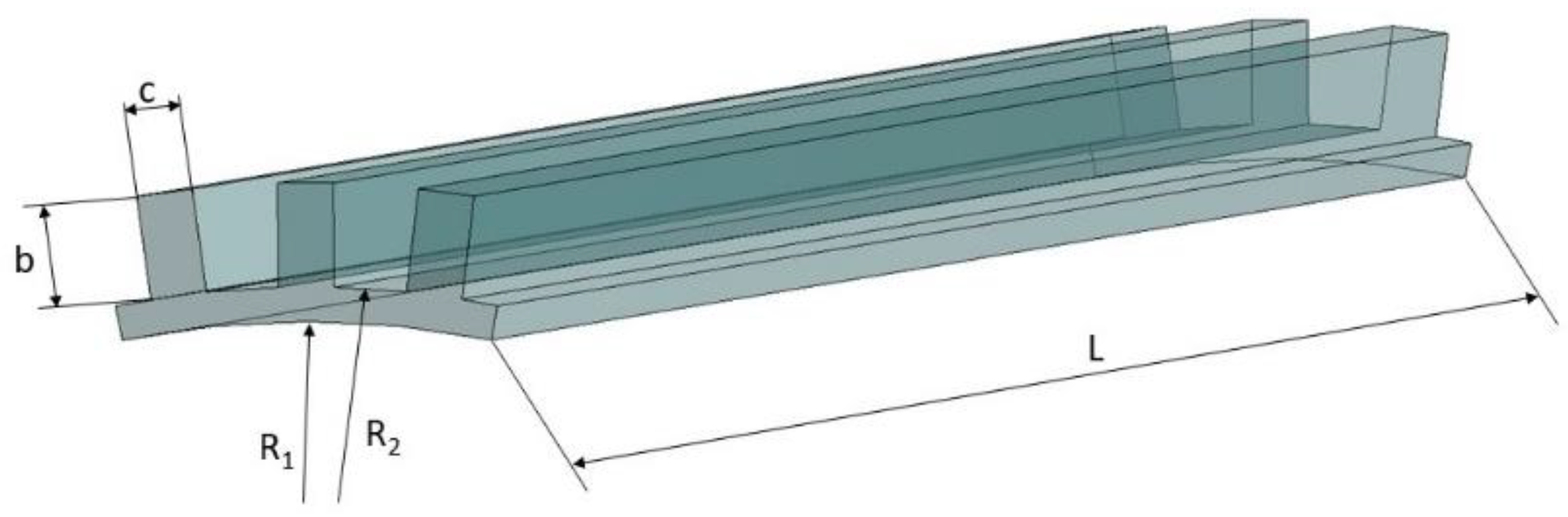
2.1.1. Geometry Parameters

An air-gap geometry is described with three non-dimensional parameters. The first is the aspect ratio of rotor and stator radii η = R 1 / R 2 . The second is the axial aspect ratio Γ = L / ( R 2 R 1 ) . The third is particular to grooved air gaps and describes the ratio between groove height and width, γ = b / c . The number of grooves is defined as N g .
Important geometry parameters for flow and heat transfer are the hydraulic diameter D h and the reference heat transfer area S m . The common definition, D h = 4 A / o , is applied for the first, while the second is obtained as S m = 2 π R m L . Definitions follow from [7,11]. It is important to note that the definition of the mean radius R m is different for smooth and grooved gaps. The two resulting definitions for R m are given with Equation (1). Both definitions use a common basis, though the B parameter represents the equivalent gap height for grooved gaps, and thus replaces the difference R 2 R 1 .
R m = R 2 R 1 ln η 1 ;   R m = B ln R 1 + b R 1 .

2.1.2. Flow Parameters

Axial R e a x , tangential R e τ Reynolds and Taylor T a numbers are the main parameters that characterize the flow. Reynolds numbers R e a x and R e τ describe the ratio between axial or rotational inertia and viscous forces. Together, they form the effective R e e f f number. The definitions of all three Reynolds numbers are provided with Equation (2). The value of c coefficient is chosen as 0.5, following [12].
R e a x = u D h ϑ ;   R e τ = Ω R 1 D h ϑ ;   R e e f f = R e a x 2 + c ( R e τ ) 2   .
The Taylor number describes the ratio between centrifugal and viscous forces. Its definition differs considerably between various sources. The definition, which takes into account η and R m , and is listed for instance in [7], is used in this paper, since it is transferrable between smooth or grooved gaps. The definition of the Taylor number is given with Equation (3):
T a = Ω 2 R m ( D h 2 ) 3 ϑ 2 1 F g ;   F g = ( π 4 / 1697 P ) ( ( R 2 + R 1 ) / ( 2 R 1 ) ) .
P = 0.0571 ( 1 0.652 ( R 2 R 1 ) R 1 ) + 0.00056 ( 1 0.652 ( R 2 R 1 ) R 1 ) 1 .
An additional flow parameter is the friction factor. This provides information about pressure losses at certain axial flow velocities, and is defined with Equation (5):
f = 2 D h L Δ p ρ u 2 .

2.1.3. Heat Transfer Parameters

The Nusselt number N u , defined with Equation (6), is applied to characterize the magnitude of convective heat transfer under certain conditions in an air gap:
N u = α D h λ .
This definition applies to global and local heat transfer. Crucially, the definition of α differs between TC and TCP flows. When considering TC flow, it applies the temperature difference between the rotor and stator Δ T = | T 1 T 2 | , following remarks in [11] and the definitions in Bouafia [7]. For the TCP flow, the difference between a surface and bulk fluid temperature, Δ T = | T 1 , 2 T b | , is used. The value for α is obtained with Equation (7):
α = Q ˙ S m Δ T = q ˙ Δ T .

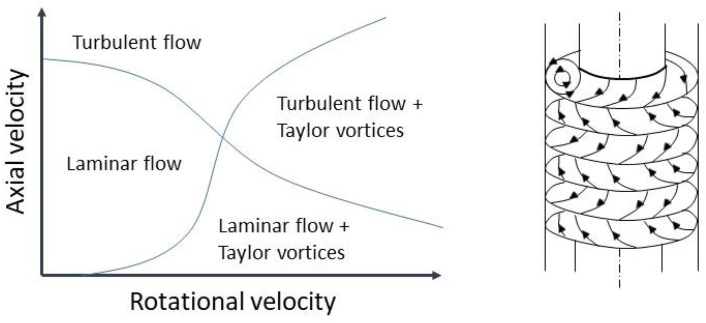
2.2. The Variability of the Flow and Heat Transfer Phenomena in an Air Gap

The flow and heat transfer phenomena that can appear in air gaps are difficult to predict. However, focusing on them is not the key to constructing adequate 3D CFD models. Instead, the focus should rather be on the definition of the underlying flow characteristics that can be used as indicators of certain flow phenomena. In order to determine these characteristics, the flow phenomena are divided into developed and undeveloped flow groups; this division allows for a more structured view. The first group represents the reference flow phenomena that are particular to air gaps and are also most often researched. The second group represents the flow phenomena that affect the appearance of developed flow, and thus introduce additional complexities. Descriptions of the main flow and heat transfer characteristics are provided first for developed and then for undeveloped flow groups. The underlying flow characteristics from both are then consolidated.

2.2.1. Flow Phenomena and Their Impact on Heat Transfer in Developed Air-Gap Flows

Developed air-gap flows exhibit one of the four main flow modes illustrated in Figure 1. The various apparent flow phenomena appear depending on the imposed TC or TCP flow conditions. However, the R e a x and T a values at which these modes appear vary between different air gaps. The appearance of Taylor vortices must be considered first, since they introduce a strong radial velocity component and result in a notable heat transfer increase. Their appearance is marked with a critical T a c r number, which changes due to geometry and flow conditions. In the reference smooth and narrow ( η 1 ) air gap with TC flow, this usually equals T a c r = 1800 [11]. In case of TCP flow, T a c r increases with increases in axial velocity. This is not monotonic, as Gardiner [5] reports that for very high T a numbers, R e a x does not affect the appearance of Taylor vortices. The presence of grooves also increases T a c r . The most often mentioned value is, following Fénot [11], T a c r = 3900 . However, T a c r decreases when N g increases [13]. A similar effect on T a c r is imposed when the gap narrows [11]. It is thus difficult to predict when these vortices appear in a certain air gap. Their detection is, on the contrary, easier. They always appear in the form of coherent, counter-rotating pairs of vortices, which distinguishes them from other vortex structures. However, the detailed characteristics of Taylor vortices can vary. As presented thoroughly in experiments by Wereley, first in [29] and then in [30], as well as by Lueptow [31], Taylor vortices can vary in size and orientation in the tangential direction, depending on the rotational and axial velocities in the air gap. As a result, Taylor vortices can also express a steady or transient nature.
The second important flow mode is represented by turbulent flow, which introduces turbulent vortices and fluctuations to the flow. Although it has a positive effect on convective heat transfer, the review by Fénot [11] states that its appearance is not as well described as the appearance of Taylor vortices and, especially in TCP flows, depends on multiple factors. There also exists no sharp limit at which turbulent flow appears, which holds for the transition to turbulent flow with Taylor vortices as well. Nevertheless, some directions can be obtained. For the reference case of a TC flow in a smooth air gap, Fénot [11] quotes that the flow becomes fully turbulent, and is without Taylor vortices above T a = 1300   T a c r . However, turbulent flow with Taylor vortices does appear at much smaller T a values. Axial velocity becomes an important parameter in the transition to turbulent flow. The values of R e a x between 1500 and 2000 are present in various reported results in Fénot [11], as the values where transition to turbulent flow occurs. Following the graph in Figure 1 as well as the results in Fénot [11], these values often decrease with increases in T a . Finally, the geometry has a crucial role in the appearance of turbulent flow as well.
The presence of turbulent flow or Taylor vortices inherently answers the question of whether the remaining two main flow modes and their specific flow phenomena are present. In terms of their impact on heat transfer, it should be added that laminar flow leads to the lowest heat transfer. On the other hand, the literature, especially the results of Gardiner [5], show that Taylor vortices introduce a higher increase in heat transfer than turbulent flow. The correct capture of the presence and transition between the flow modes in developed air-gap flow is thus crucial for establishing the validity of 3D CFD models.

2.2.2. Flow Phenomena and Their Impact on Heat Transfer in Undeveloped Air-Gap Flows

Although the developed flow presents the reference, it appears only at a certain distance from the air-gap entrance. In TCP flow cases, it can also happen that the gap length is too short to allow developed flow to establish [11]. An entrance region is thus present. This features a gradual development of the average velocity profile, together with the possibility for appearance of a recirculation zone, and to it connect vortical structures that are near the entry to the air gap. The resulting variety of combinations between the entrance region and developed flow phenomena consequently increase the complexity of air-gap flows.
The presence and size of the entrance region is affected by the geometrical parameters and flow conditions that are in the vicinity of the air gap as well. Accurate air-gap flow modelling thus requires definitions of conditions outside of the air gap. Some general trends are nevertheless indicated in the literature. Results in Maud [24] and Haddadi [22] reveal that the entrance region length increases with increases in R e a x and shortens with increases in T a . It also shortens with the presence of grooves [13]. In short air gaps, such as those studied in Lee [6], it was also noted that the presence of the entrance region determines flow conditions, except for high T a values where Taylor vortices appear.
The entrance region was also found to increase the heat transfer [11]. Crucially, the appearance of Taylor vortices still enables further increases in heat transfer, as shown in the results of Lee [6]. These vortices appear only at suitably high T a values, while the entrance region can otherwise affect velocity conditions in a considerable portion of an air gap; thus, it is important to ensure its correct modelling as well as its transition to developed flow.2.2.3. The Observed Underlying Flow Characteristics
Comparing the developed and undeveloped flow phenomena descriptions, it was concluded that three underlying flow characteristics can be used as indicators to determine the presence of certain flow phenomena, and consequently to determine related requirements for adequate 3D CFD models. The first is the presence of vortex flow structures. These are present in various sizes and shapes, from coherent Taylor vortices, to recirculation zones and random turbulent vortices. The second underlying flow characteristic is the steady or transient nature of the flow, which can be observed through the appearance of various structures as well as through the development of different variables, such as velocities at different locations. The third underlying flow characteristic is connected with the first two. This is the presence of an entrance region, which can affect both the shape and size of vortex structures, as well as local velocities along the air gap. In order to determine its presence and size, the average velocity profiles as well as flow structures from the entry to an air gap onwards can be observed.
The three defined underlying flow characteristics can be observed with little effort, using the visualization and monitoring tools in 3D CFD software. For instance, vortex structures, their locations as well as their transient or steady nature can be visualized with the plots of λ 2 iso-surfaces [32]. The transient or steady nature of the flow can be determined also by monitoring local values or various variables as well as the velocity profiles along the air gap. These, together with observations of the present vortex structures, can help in defining the size and impact of the entrance region. Having this possibility to identify and observe the underlying flow characteristics is crucial for the development of the workflow.

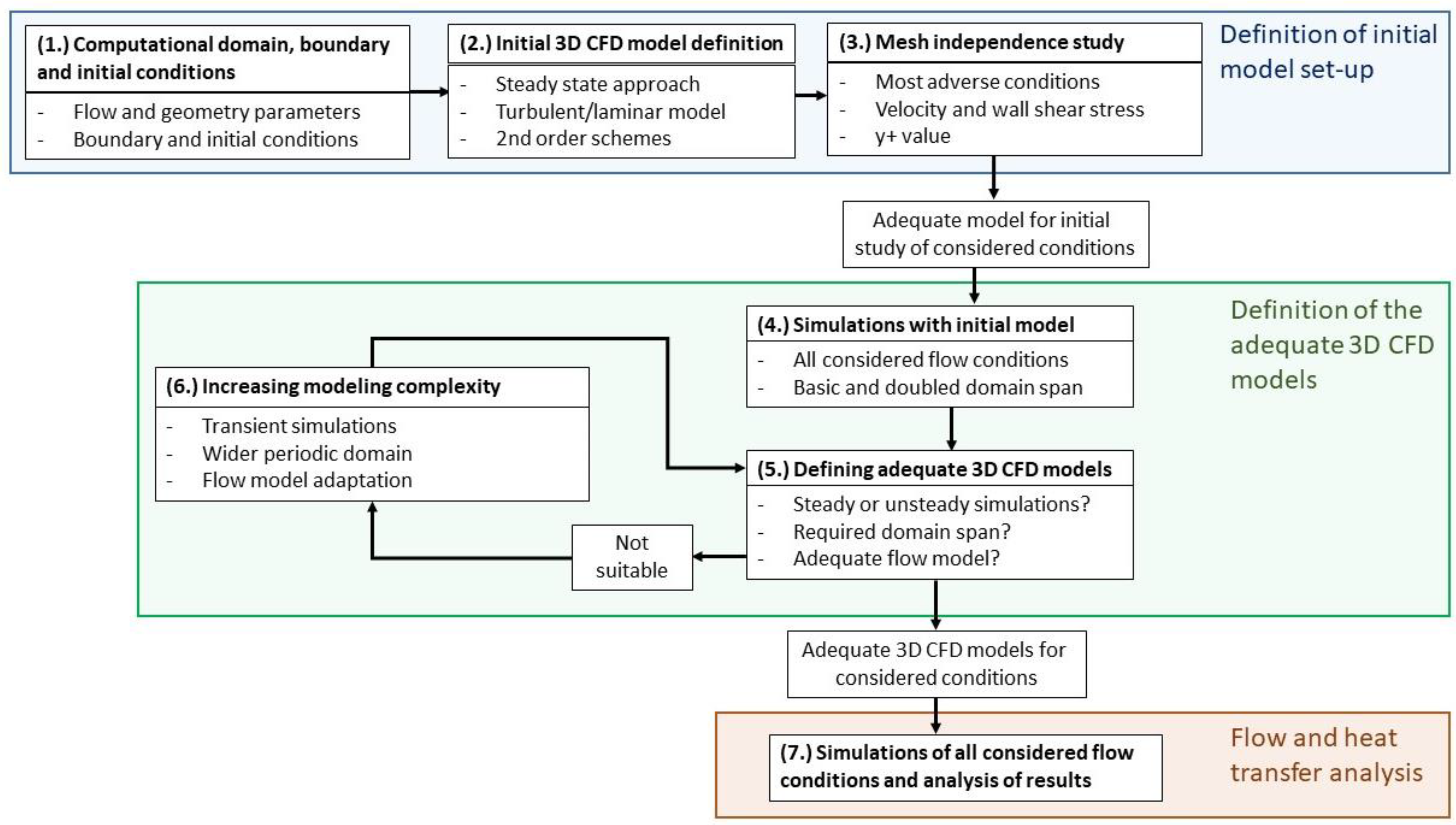
2.3. The Workflow for Definition of Adequate 3D CFD Models

The proposed workflow aims at defining adequate 3D CFD models for imposed conditions in an observed air gap by identifying the presence of the underlying flow characteristics. Three fundamental questions were formed following the discussion on these characteristics, in order to aid in their identification:
(1)
Is there turbulent or laminar flow present?
(2)
Is the flow at observed operating conditions steady?
(3)
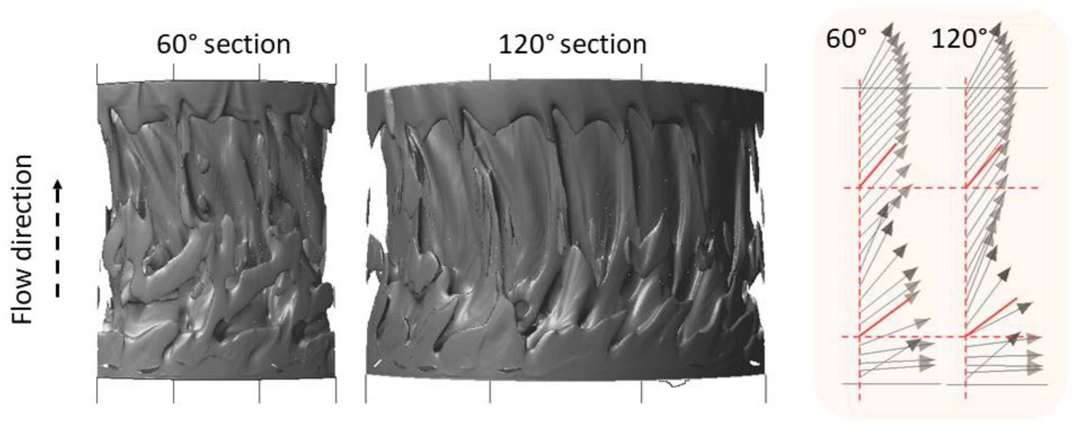
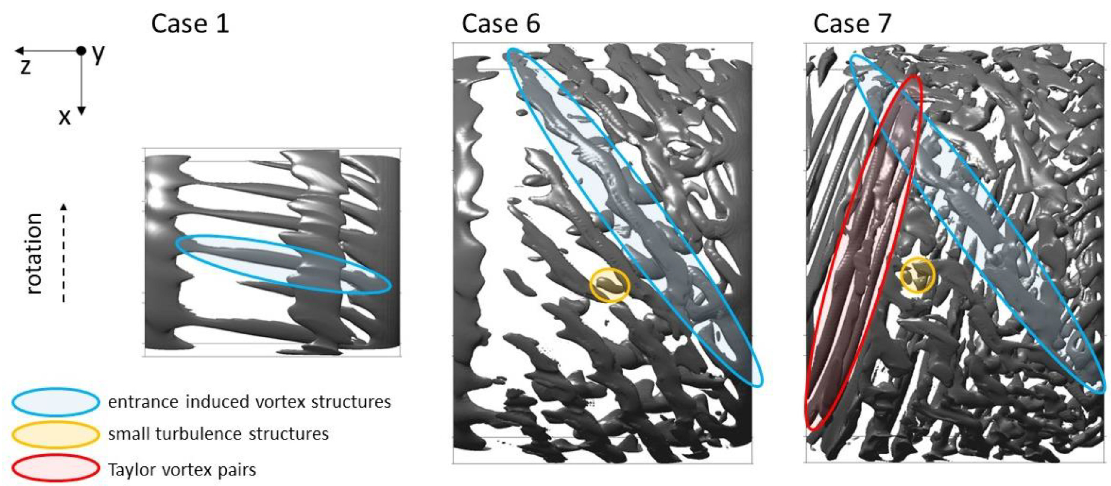
Are vortex structures present, and what is their size range and span in the azimuth direction?
The workflow was constructed by applying these questions to results that were obtained from 3D CFD simulations. If analysis points towards the presence and importance of a certain characteristic, further steps to introduce its improved modelling can be made.
The constructed workflow is presented schematically in Figure 3. It is composed of three main groups of steps, through which an adequate 3D CFD model for an observed air-gap flow is defined. The first group presents a definition of the initial 3D CFD model, which provides the basis for construction of the adequate model. The second group of steps applies this basis in simulations of all considered conditions in the observed air gap. In addressing the three aforementioned questions, the underlying flow characteristics are defined, and the 3D CFD models are adapted accordingly. This is performed in an iterative loop, in which the accuracy of the models gradually improves until adequate models are obtained. With these, the last step is performed. This includes the final simulations of considered flow conditions, and analysis of the results.
The following subsections describe and explain the workflow steps in each of the three groups in detail. As the workflow includes manipulation with modelling set-up, it requires a suitable construction environment. Ansys Workbench version R19.2 [33] was applied, while simulations in it were performed using CFD software Fluent [34].

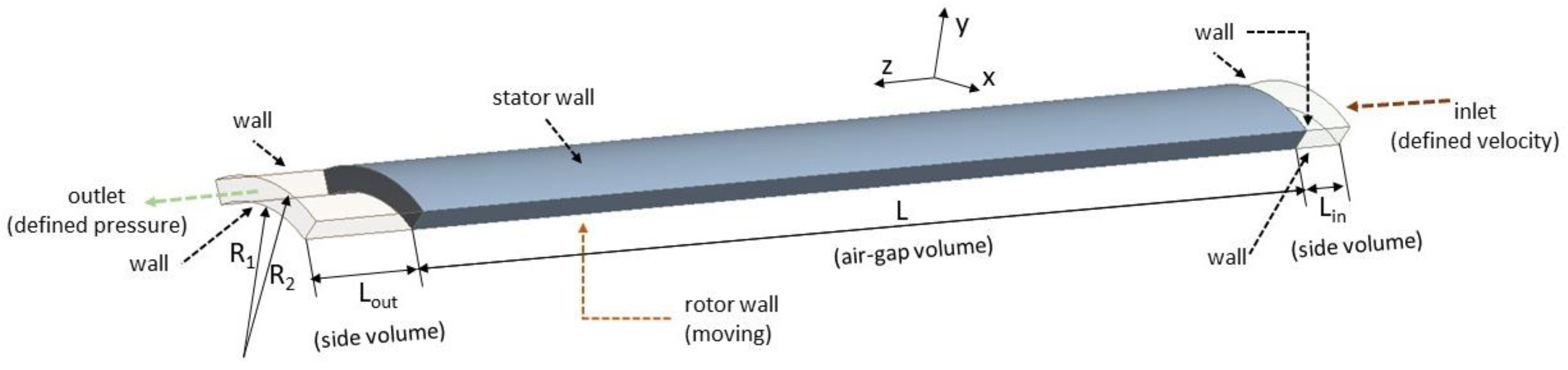
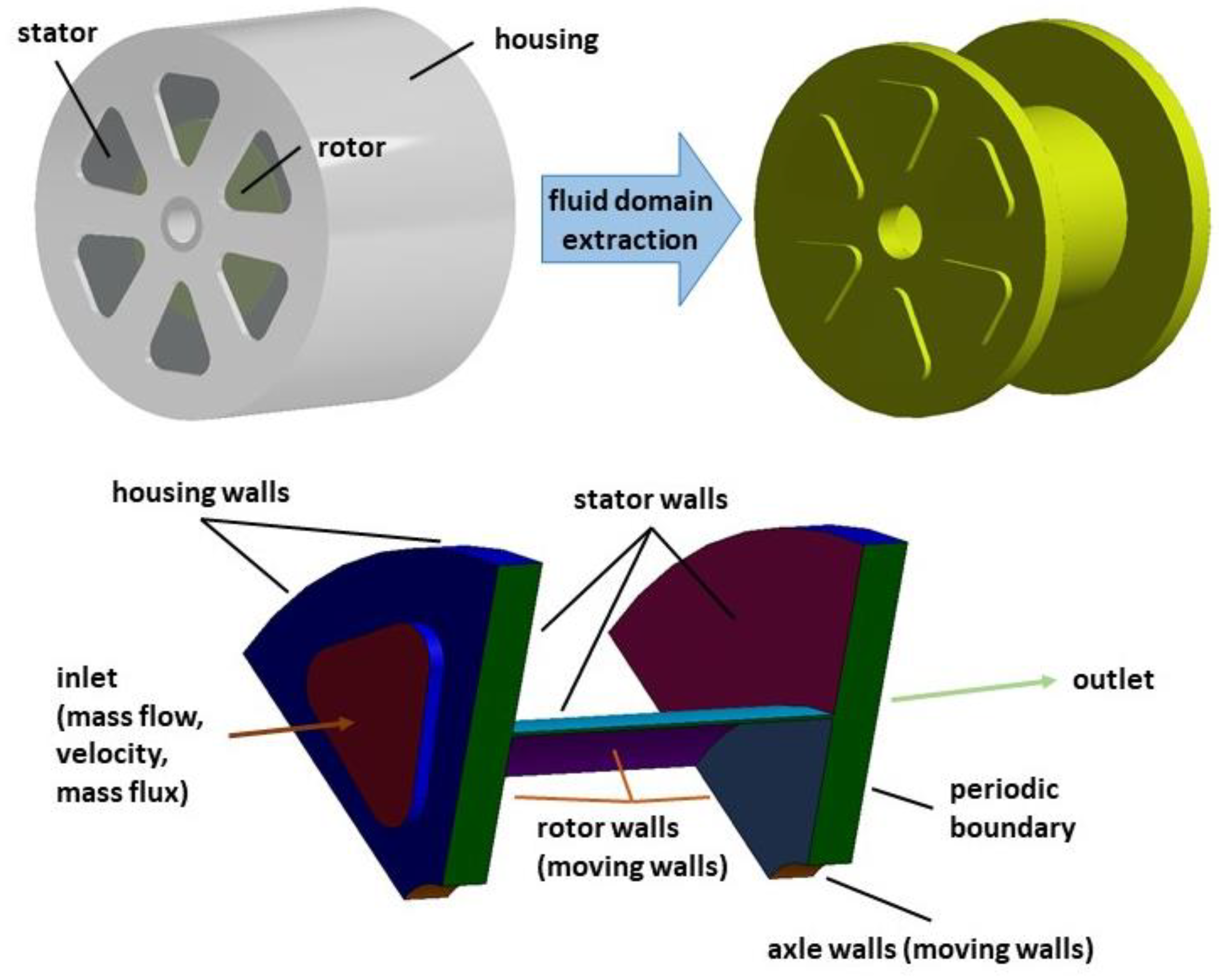
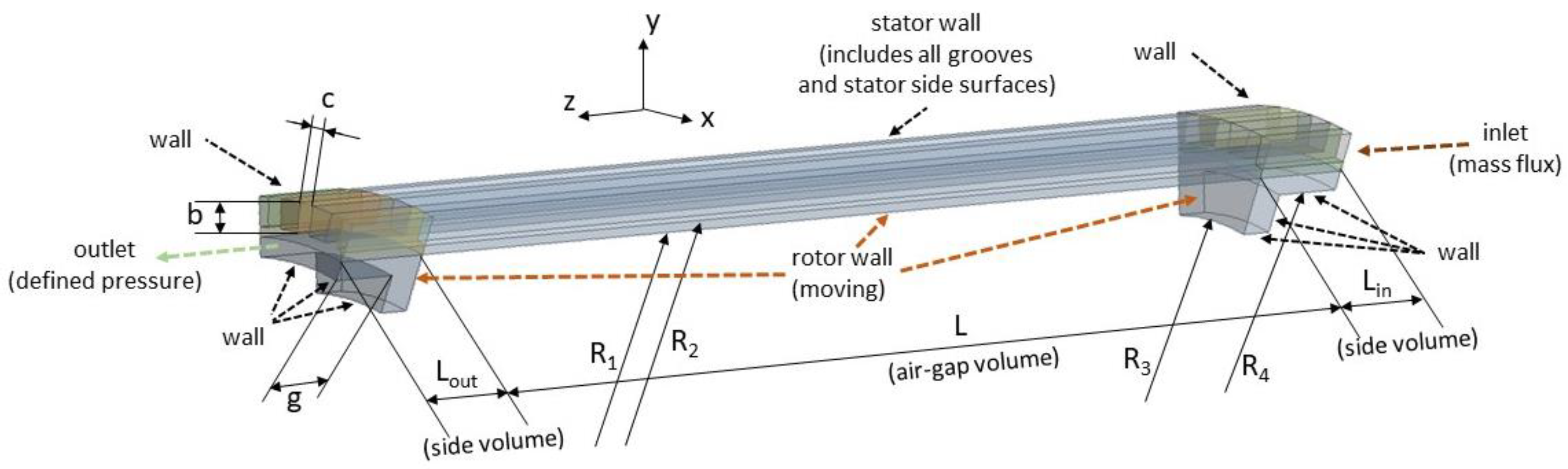
2.3.1. Definitions of Computational Domain, Boundary and Initial Conditions (Step 1)

The first step deals with the fundamental definitions that are required to construct the 3D CFD model. These are presented in the following subsections.
(a)
Computational domain
The computational domain includes both the air gap and its surrounding volume, in order to ensure that the air-gap entrance region as well as its impact on the air-gap flow are adequately modelled. An example is depicted in Figure 4, where the computational domain features the fluid domain that spans from the inlet to the outlet of the observed EM. Note that the computational domain includes only a section of the whole domain in the azimuth direction. This lowers computational costs, but requires adequate definition of the domain span. The guidelines on periodic wall-bounded flow simulations, stated for instance in [35], are considered. These guidelines require that velocity correlations between the periodic limits should disappear, which translates to the need for an unobstructed development of flow structures. Thus, the domain size must be several times larger than the size of the largest flow structures [35]; the suggested domain spans for the considered air gaps were defined following this. Due to the simple shape and expected lower number of cells, the smooth air-gap models should feature a 60° span. As this is a relatively large span, especially compared to available numerical works, it ensures a higher possibility of unobstructed development of vortex structures in the tangential direction, supporting their more reliable identification. A smaller angle is preferable for grooved air gaps, which is a result of optimizing computational costs due to an expected higher cell number caused by the presence of grooves. At least two grooves are included to capture the potential presence of flow structures that are wider than one groove. This is contrary to most of the available literature, where only one groove is included, as in the studies by Bouafia [19] or Lancial and Torriano [27].
(b)
Boundary and initial conditions
The applied boundary conditions follow the conditions in the considered EM. Their illustration is shown in Figure 4. The walls that are connected with the rotor and axle are defined as moving walls that have a certain angular velocity Ω , defined from the T a value. All walls are otherwise defined as no-slip walls. In terms of thermal boundary conditions, the walls can be either adiabatic, heated with certain heat flow or temperature, or have a prescribed thermal resistance that is combined with thermal conditions outside the EM. Thermal conditions are also set according to the considered EM.
Although depicted in Figure 4, the inclusion of inlet and outlet boundaries is necessary only for TCP flow cases. Their definitions are affected by the surrounding volume of the air gap. As the flow develops and enters the air gap from this volume, it is not necessary to define the exact velocity profile of the domain inlet. This alleviates the question concerning how to impose adequate air-gap entrance conditions, which can, following remarks in Fénot [11], also affect heat transfer phenomena. Definitions of mass flow, mass flux or average velocity, together with the temperature of the domain inlet are sufficient. The inlet turbulence properties, such as turbulent intensity, length scale, kinetic energy, etc., have to be prescribed, but are not crucial for the air-gap flow development, which agrees with observations in [24]. Outlet is defined as the pressure outlet. In the case of TC flow, a reference value for the system pressure field is defined. This pressure is preferably defined in a location where its value is known. Finally, the two side surfaces that limit the domain in the azimuth direction are defined as periodic boundaries.
The applied boundary conditions also relate to initial conditions. In the case of mid–high R e and T a values, it was found that convergent simulations may require application of a gradual increase of imposed rotational and axial velocities. Thus, the initial conditions impose velocities that are in the range of laminar or weak turbulent flows. These are then increased in a step-wise manner to the final, desired velocities. The same approach is applied for thermal boundary conditions, where higher temperature differences or heat flow on heated surfaces are achieved in a step-wise manner.

2.3.2. Initial 3D CFD Model Definition (Step 2)

The role of the initial 3D CFD model is to provide a sound foundation for the identification of underlying flow characteristics in the considered air gap. The initial model is constructed as a combination of models and settings that are most often applied in the reviewed literature and, on average, return mostly valid results. The initial model thus presents the common point from which all 3D CFD models, that are defined with the workflow for different operating conditions, are built.
The flow is modelled by resolving the NS continuity, momentum and energy conservation equations; these are listed in respective order with Equations (8)–(10).
ρ t + · ( ρ v ) = 0
( ρ v ) t + · ( ρ v v ) = p + · ( μ ( ( v + ρ v T ) 2 3 · v I ) )
( ρ e 0 ) t + · ( ρ v e 0 ) = p v + · ( λ T + v μ ( ( v + ρ v T ) 2 3 · v I ) )
The listed set of equations requires an additional equation of state to be closed. This is defined by assuming that the air is an ideal gas. It must also be considered that the flow in the air gap might be laminar or turbulent. The estimation if a turbulent flow is present follows from the R e and T a numbers. For laminar flow, no specific adaptations are required, and the above listed equations are solved. In the case that the flow is turbulent, RANS turbulence modelling is applied, based on the Reynolds-averaged forms of Equations (8)–(10). The initial 3D CFD model applies the k ω SST turbulence model. The model introduces two additional transport equations, one for turbulent kinetic energy k , and one for specific dissipation rate ω . These equations are listed with Equations (11) and (12), in accordance with [34], where a more detailed explanation of their terms may be obtained.
( ρ k ) t + · ( ρ v k ) = · ( Γ k k ) + G k ˜ Y k
( ρ ω ) t + · ( ρ v ω ) = · ( Γ ω ω ) + G ω Y ω + D ω
The k ω SST model was chosen, as it was found to be the most adequate in publications where different turbulence models, including LES models, were compared, either in TC flows [27] or in adiabatic [24] and diabatic [3] TCP flows. It provides an improved description of wall-bounded flows as well as of low R e number flows [34], which are often present in air gaps. In line with this, it also applies the near-wall modelling approach. This corresponds to the need for accurate velocity and temperature profiles at the walls.
The initial 3D CFD model also assumes the flow to be steady. This was found to be adequate in performing initial simulations, including those at high R e and T a values, and is backed by available numerical studies, notably [3,24,28].
The solution to coupled Navier–Stokes equations for continuity, momentum and energy is obtained via the SIMPLE algorithm. The least squares cell-based discretization is applied to resolve gradients, with the pressure gradient term defined by a second-order scheme. Other quantities in Navier–Stokes and turbulence model equations are defined with second-order upwind schemes.

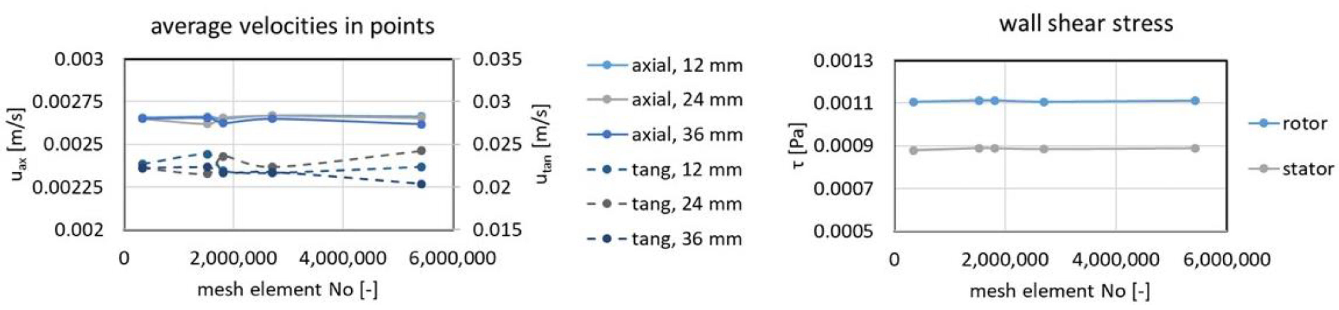
2.3.3. Mesh Independence Study (Step 3)

The necessary prerequisite for convergent steady state simulations at various R e and T a values is also the use of an adequate mesh. Definition of such a mesh is obtained with the mesh independence study. In it, simulations featuring successively refined meshes are performed until certain key results no longer change [36]. This allows for the elimination of discretization errors that originate from the size of mesh elements, and helps to ensure convergent simulations [36]. The goal here is to define one adequate mesh for all considered flow conditions in the air gap. The most adverse flow conditions are thus simulated with the initial model. The suitability of this approach follows from the fact that the highest gradients in flow are present in the entrance region, on the rotor surface and at sharp edges of stator grooves. Being locally constrained, they do not depend on the domain span, and are shown to not change considerably if flow is treated as unsteady.
The applied meshing approach imposes the structured mesh in the air gap and the unstructured mesh in the remaining outside volume. This simplifies meshing of the complex outside geometry, and introduces high-quality and computationally efficient meshes in the air gap. Suitably refined meshes are defined via comparisons of results for different variables on gradually refined meshes. These variables are the average values of velocity components at multiple points in the air gap as well as wall shear stress values on the rotor and stator. Since the model is focused on valid heat transfer descriptions, which require well resolved temperature profiles, the average y + value of the first cell layer on rotor and stator are also compared. The suitably refined mesh on rotor and stator requires the average value y + < 1 . This is in agreement with mesh refinements found in other papers such as in Hamidi [3], and in Lancial and Torriano [27].

2.3.4. Defining Adequate 3D CFD Models for Observed Flow Conditions (Steps 4, 5 and 6)

The initial 3D CFD model is fully set after the definition of an adequate mesh, and can be applied in the search for adequate 3D CFD models for the considered conditions. Thus, simulations of all considered flow conditions in the air gap are first performed with it. This is listed as step 4 in the proposed workflow scheme. Importantly, two groups of simulations are performed, one with the initially set domain span, and the other with the doubled span. This is primarily done to determine whether the initially defined domain span allows for unobstructed development of the flow. Furthermore, on the basis that this difference can affect flow development, it provides additional data for finding the answers to the three fundamental questions and, through them, the definitions of adequate 3D CFD models. This analysis is presented in the following subsections, and is listed as step 5 of the workflow.
(a)
Should steady or unsteady flow modelling be applied?
Determining whether steady state modelling is suitable or not follows from the observations of local results for various variables, most notably velocity, over a longer interval of iterations. The interval has to present the already converged state, in which residuals are not decreasing further. The notable variations in these values, most often periodical over iterations, point to the presence of unsteady flow conditions. Additionally, contours of velocity field, λ 2 iso-surfaces and pathlines at different iterations can be observed, in order to determine potential local flow unsteadiness.
Apart from the listed variables, it was also found that the relative standard deviations of local velocity, wall shear stress and heat transfer can serve as flow steadiness identifiers. Their definitions are provided with Equation (13). In this, Ψ R S D denotes the relative standard deviation value, while Ψ i and Ψ ¯ represent the instantaneous and average values of a certain variable during N iterations after a converged state is reached.
Ψ R S D = i = 1 N ( Ψ i Ψ ¯ ) 2 N 100   [ % ] Ψ ¯ .
Comparing Ψ R S D values with results observed during simulations, it was found that unsteady simulations should be performed when Ψ R S D > 3 % . This can be applied for more streamlined definitions of whether the flow can be described as steady, or if transient modelling is suitable.
The adequate time step size must be defined if the need for unsteady simulations is confirmed. The Courant number C is used for this. Its definition is provided with Equation (14), as follows:
C = U Δ t Δ x .
U represents the velocity magnitude, defined as U = u a x 2 + ( Ω R 1 ) 2 , while Δ x and Δ t represent the cell size in axial or tangential direction and time step size. The time step in this study is defined in order to impose C < 3 . This ensures that C values are overall well below the recommended highest values in Ansys Fluent [34], which are stated to be in the range from 20 to 40.
(b)
Defining the adequate domain span
Determining whether the initially proposed domain span is adequate or a larger span is required relies on the observation of two criteria, which are directly related to the development of flow in the azimuth direction. The first is the development of flow structures. Iso-surfaces of the λ 2 criterion are used for this. The domain span can be considered adequate if there is no difference in the appearance and development of various vortex structures in the flow between the two applied domain spans. The second criterion is the angle between the flow and axial direction. The indication to use a wider domain is found in the difference in this angle between the two applied domain spans. Velocity vectors or pathlines are observed to determine this angle, and with it the need for a wider domain. An example of how the domain span affects flow development, and how the vectors and structures are used to identify the adequate domain span, is provided in Figure 5. This depicts turbulent TCP flow in a smooth air gap at R e a x = 1500 and T a = 546,300 . It is clear that the flow structures and vectors share many similarities. However, the flow structures in the two domains clearly evolve in a different manner. The average velocity vectors confirm this difference, as the angle between them and the axial direction is not the same as that between the initial and doubled domains. This is represented with the red lines in Figure 5, which depict the vector directions in the initial domain. A wider domain span is thus necessary in this particular case.
(c)
Defining the adequate flow model
The EM air gaps are narrow, and can thus in many cases feature laminar or only weakly turbulent flows. The appearance of vortex structures as well as the ratio between turbulent and molecular viscosity υ T / υ are observed to estimate if turbulent flow is present, and thus if the turbulent model is required. In the case of there being only large vortex structures pointing to recirculation zones, and low viscosity ratios are reported, the flow may be laminar, and the laminar flow model could be more adequate. It has to be also acknowledged that transitional flow models, such as intermittency models [37] which describe the transition from laminar to turbulent flow, could also be applied. The suitability of their application and use is, however, not the topic of the present study, but remains an interesting field for future work, in addition to the use of more accurate hybrid RANS–LES and LES models.
The 3D CFD models are adjusted on the basis of the result analysis that identifies the presence of underlying flow characteristics. Either unsteady simulations, wider domain or different flow models can be applied to ensure that modelling of these characteristics as well as their associated connected flow and heat transfer phenomena are improved. However, each model change has to be verified, as it is possible that a further increase in the domain span or a change in the applied flow model is required. Thus, a new set of simulations must be performed, calling for repeated analysis of results, leading to the loop that is shown in Figure 3 and features steps 5 and 6.

2.3.5. Simulations with Adequate 3D CFD Models and Results Analysis (Step 7)

The developed workflow gradually increases the complexity of applied 3D CFD models through a thorough analysis of the intermediate results. In return, improved modelling of all relevant flow phenomena is ensured, which provides a solid foundation for valid flow and heat transfer valorization in a certain air gap. This is done using defined adequate models for a complete range of considered conditions, and represents the final step of the workflow. Importantly, since an adequate model is defined for each considered flow case, the unnecessary overall application of unsteady simulations or a larger domain is avoided. The computing costs are thus lowered, and results are obtained more quickly and efficiently.

3. Results

The following subsections demonstrate the use of the proposed workflow through its application in three different cases. The chosen cases are defined from the available literature, in order to enable thorough validation of the results. First, a smooth air gap with laminar TCP flow and a specific shape of Taylor vortices is considered. Then, turbulent TCP flows in a short and smooth air gap are studied to illustrate how entrance region effects are captured. Finally, a grooved air-gap configuration with turbulent TCP flow is presented, where the goal is to produce a description of the local heat transfer along the air gap.
All cases are presented through the main steps of the workflow, from the definition of the computational domain and boundary conditions, to the analysis of the results obtained through the generated adequate 3D CFD models.

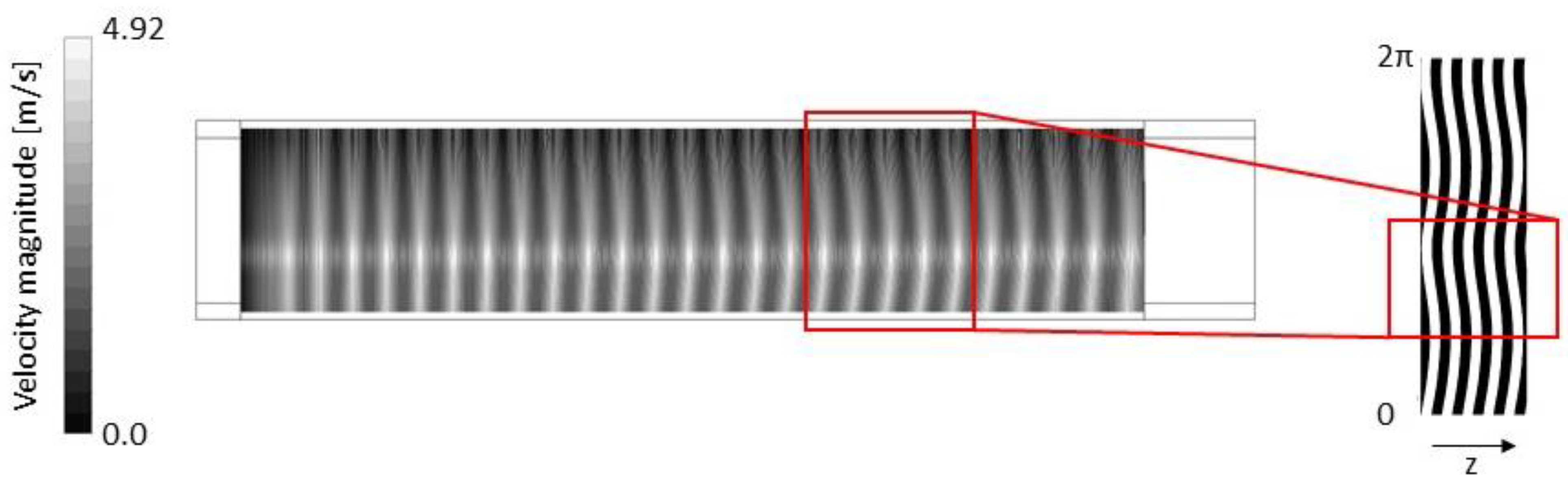
3.1. Laminar TCP Flow with Wavy Taylor Vortices

Wavy Taylor vortices are a specific form of Taylor vortices. They impose unsteady flow, where the wavy shape stretches across a certain domain span. Thus, modelling such vortices allows us to validate the workflow in terms of its ability to identify the need for unsteady simulations as well as an adequate domain span. The case definition relies on the experimental research presented in Wereley [30], while validation applies results of numerical simulations to those produced from Hwang [21], which also modeled the conditions observed in Wereley [30].

3.1.1. Definition of Computational Domain and Boundary Conditions (Step 1)

As set by the workflow, the computational domain and flow conditions are first defined. The computational domain is presented in Figure 6 with the indicated main dimensions and boundary conditions. The domain follows from the description of the experimental apparatus in Figure 1 in Wereley [30]. This features a long and smooth air gap to ensure the appearance of developed flow, in which the Taylor vortices are observed. The side volume on the inlet side is shaped as an extension of the air gap, and features well-conditioned flow through the use of laminators. The side volumes on both sides of the computational domain were thus defined as extensions of the air gap. The computational domain was defined as a 60-degree section of the whole air gap, in accordance with the workflow definitions regarding the use of periodic boundary conditions. The dimensions and geometrical parameters that describe the defined domain are listed in Table 1.
Flow conditions are defined with the pair of R e a x and T a values at which wavy vortex flow was observed in Wereley [30]. Their values are given in Table 2 and determine the applied rotational velocity of the rotor surface Ω and the axial velocity on the inlet u . Other walls are treated as stationary. All walls are in terms of thermal boundary conditions treated as adiabatic, which follows from the experimental conditions. Air at 293 K is introduced at the inlet, which is different from the experimental conditions in Wereley [30]. These featured a mixture of water, glycerol and sodium iodide due to PIV visualization. The outlet is set as a pressure outlet with p = 1   bar .

3.1.2. Initial 3D CFD Model Definition and Mesh Independence Study (Steps 2 and 3)

The initial 3D CFD model is based on the defined computational domain, flow conditions and the settings described in step 2 of the workflow. The model thus applies steady flow modelling, second-order discretization schemes and the SIMPLE algorithm to solve the coupled system of Navier–Stokes equations. As the low R e a x and T a values clearly point to the presence of laminar flow, the laminar flow model is applied. Air is modelled as an ideal gas, although the adiabatic conditions allow for the use of the incompressible gas assumption.
The simple geometry allows for the structured mesh to be applied throughout the computational domain. The mesh independence study, which presents the third step of the workflow, is performed to determine the adequate meshing. Applied meshes include from 3.43 × 10⁵ to 5.43 × 10⁶ cells. The study is performed at the listed R e a x and T a pair. Observed variables are average axial and tangential velocities in three points at mid air-gap height, located at 12, 24 and 36 mm from the air-gap entry. Additionally, wall shear stresses on the rotor and stator are observed. The obtained results are provided in Figure 7. From them, it was determined that the adequately refined mesh features 2.7 × 10⁶ elements, and is set as defined in Table 3.

3.1.3. Definition of the Adequate 3D CFD Models (Steps 4, 5 and 6)

While the laminar flow model is the adequate choice due to low R e a x and T a values, there remain questions about whether the unsteady flow description is required and what the adequate domain span is. In order to obtain the answers, steady state simulations with the initial model, featuring the initial and doubled domain spans (60° and 120° in the azimuth direction) were performed initially, in accordance with step 4 of the workflow. The analysis of their results, which represents step 5 of the workflow, initially deals with the question of flow steadiness. The graphs in Figure 8 present the evolution of axial velocity at the six points at mid-gap height, and at different locations from the air-gap entry after converged state is achieved. The results clearly point to the need for unsteady flow modelling. This is confirmed with the values of the relative standard deviations of the axial and tangential velocities at these same points, presented on the graphs in Figure 9.
The definition of an adequate domain span is considered next. For this, the λ 2 iso-surfaces in the two domains were compared. Their plots are shown in Figure 10. Clearly, their vortex structures are very similar. However, there is a presence of slightly wavy Taylor vortex pairs in the second half of the wider domain. This agrees with the differences in the reported relative standard deviations shown in Figure 9, which indicate considerably different variability in the flow in the wider domain. The larger domain span thus seems to allow for an additional degree of freedom, and affects the development of flow structures.
The analysis of obtained results indicates a need to apply changes to the initial 3D CFD model. Unsteady simulations with a time step of Δ t = 0.02   s were introduced. The time step size leads to highest Courant number of 1.3. A wider, 120° span was applied due to the reported observed differences in the vortex structures and deviations. Initialization with results from the steady-state simulation was applied, after which the simulation ran until periodic results were achieved (40-s flow time). The results obtained with the adapted model were again analyzed, as proposed by the workflow. It was found that the applied adaptations indeed lead to the appearance of the wavy Taylor vortices. Since it was unclear if an even wider domain span would lead to further development of the wavy vortex form, an even wider 180° domain span was tested. This is in line with the constructed workflow and the imposed loop between steps 5 and 6. As this wider domain was not found to result in further changes, it was determined that the adequate 3D CFD model includes a 120° domain span and unsteady flow modelling. The results, obtained during the definition of the adequate model, are also the final results. They are discussed in the next section.

3.1.4. Analysis of Final Results (Step 7)

The final results are presented in Figure 11 with a depiction of the obtained Taylor vortices. These show that the wider domain allows for the development of instabilities in the azimuth direction, from which the wavy Taylor vortices appear. They appear only in the second half of the air gap, which corresponds to statements in Wereley [30], where it is mentioned that the various forms of Taylor vortices are observed only in the developed flow region.
The validated numerical results of Hwang [21], which model the wavy vortex flow observed in Wereley [30], are also presented in Figure 11. The reason for this is that a more thorough, yet compact validation can be given with them, than with results depicted in Wereley [30]. Namely, comparing the Taylor vortices from the adequate 3D CFD model with those from Hwang [21] (the red rectangles) shows that they are practically identical. Both the size of a vortex pair as well as its wavelength match, which inherently points to the overall correspondence of velocity fields, and hence validity of results.
The case depicts how the valid description of flow phenomena is gradually achieved from following the workflow steps. Furthermore, it should be noted that in Hwang [21], a complete domain span is applied, as shown in Figure 11. In line with the fact that only a portion of the domain in the axial direction is shown for the results from Hwang [21], it also follows that the proposed workflow defines a more optimal simulation set-up. Computational costs can be assumed to be three times lower, considering that only one-third of the domain span is included in the model that was obtained with the workflow.

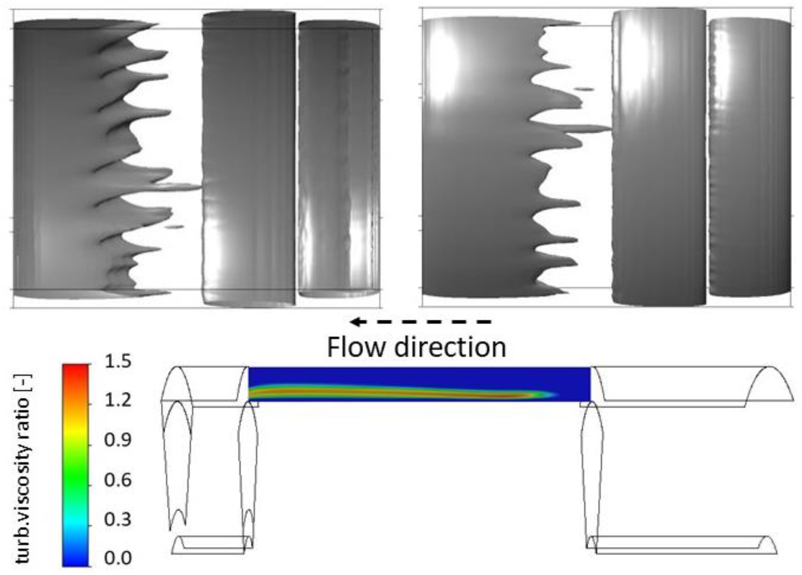
3.2. Turbulent TCP Flow in a Smooth and Short Air Gap

This case provides validation of the workflow in regards to capturing entrance region effects as well as multiple important flow phenomena that appear at the same time. It follows from Lee [6], where experimental measurements were performed in various short air gaps, and were focused on capturing the presence of entrance region effects, turbulent flow and the appearance of Taylor vortices, in addition to their effects on heat transfer.

3.2.1. Definition of Computational Domain and Boundary Conditions (Step 1)

The computational domain is based on the experimental system presented in Figure 1 in Lee [6]. The domain geometry is presented in Figure 12, together with indicated dimensions and boundary conditions. Its span equals 60°. A complex outside volume is added at both the domain entry and exit side. Its definition follows from the experimental system geometry. While the inlet is presented by the complete surface at the head (brown arrows), the outlet (green arrow) occupies only a small area at the end. The bottom of this area also determines the lowest radius of the computational domain. This configuration was adapted as it simplifies the geometry, while it does not affect the development of the flow in the air gap and hence in the entrance region also. All indicated dimensions and geometrical parameters that follow from them are listed in Table 4.
Flow and hence boundary conditions are set with a range of TCP flows at constant R e a x = 1500 and T a values between 1800 and 1.31 × 10⁶, as listed in Table 5. Their definitions follow results shown in Figure 8 from Lee [6]. The inlet boundary conditions impose a mass flux of 0.481 kg/m2s in order to ensure defined R e a x , while the rotational velocity of the rotor surfaces spans from 4.15 to 111.44 rad/s to meet the T a value range. All other walls are defined as stationary. Thermal boundary conditions also follow the observed experimental conditions. Air, modelled as an ideal gas, is introduced into the domain at 293 K. The rotor surface in the air gap is heated, and maintains a constant temperature of 323 K. All other surfaces are treated as adiabatic. The outlet is set as a pressure outlet with p = 1   bar .

3.2.2. Initial 3D CFD Model Definition and Mesh Independence Study (Steps 2 and 3)

The initial 3D CFD model is the same as the initial model in the previous case. The only difference is in application of the k ω SST model. This follows from the R e a x value, which, as stated in Section 2.2.1, corresponds to the limiting values at which the TCP flow in smooth air gaps is reported to become turbulent. Additionally, flow perturbations at the air-gap entrance are expected, which aid in the development of turbulent flow.
In terms of the applied mesh, it is important to note that Figure 12 shows the outside volume to be split into different subdomains. This allows generation of a high-quality structured mesh in the air gap, as well as improved meshing in the outside volume and near the outlet. The mesh independence study is performed as the next step. In accordance with the workflow, the initial 3D CFD model is used in simulations of the most adverse conditions, defined with T a = 1.31 × 10 6 . Gradually refined meshes with 1.5 × 10⁶ to 5.3 × 10⁶ elements are applied, and average axial velocity results at three points along the air gap as well as shear stresses on the rotor are observed. Obtained results are shown in Figure 13. The defined adequate mesh is presented with the air-gap meshing sizes listed in Table 6. The mesh applies same sizing in the outside volume. Since the flow is subjected to a direction change at the air-gap ends, the mesh features additional refinements of cells near these locations.

3.2.3. Definition of the Adequate 3D CFD Models (Steps 4, 5 and 6)

The definition of adequate 3D CFD models considers all three stated questions in Section 2.3 regarding the need for unsteady simulations, adequate domain span and use of the turbulence model. The latter is especially important for conditions at lower T a values; hence, it is the first to be considered. The case with the lowest T a value is analyzed, since, if proven adequate here, use of the turbulence model is adequate for all other cases for higher T a values. The presence and shape of vortex structures as well as the viscosity ratio υ T / υ in the air gap are observed. Their results are presented in Figure 14. Clearly, the vortex structures include recirculation zones near the air-gap inlet, in addition to distorted structures in the second part of the air gap. The latter agree with the increased zone where the υ T / υ ratio exceeds unity. Combining these observations with the limiting value of R e a x , it was determined that the turbulent flow model should be retained. Thus, all considered cases use the turbulent flow model.
The analysis in regards to the need for unsteady flow modelling and increased domain span is performed in the same manner as the previously presented case. In line with the workflow, the simulations with the initial 3D CFD model are performed with the initial and doubled domain spans. Local velocity values as well as their relative standard deviations are observed, in order to determine whether certain flow conditions require unsteady modelling; meanwhile, λ 2 iso-surfaces and vector plots are used to determine if the initial or wider domain span is adequate. It was found that for the three cases with the highest T a values, the adequate model requires application of a wider domain (120°). The λ 2 iso-surfaces and vector plots from flow case 6 are actually presented in Figure 5, as an example of using these plots to determine the need for a wider domain span. These three cases were also found to require unsteady flow modelling. For other cases, the initial model was found to be adequate. The adequate 3D CFD models for the considered cases are summed in Table 7, where the applied time step sizes in unsteady simulations and their respective Courant numbers are also provided.

3.2.4. Analysis of Final Results (Step 7)

The final obtained results were analyzed with the goal of defining global N u values on the rotor, as these values are available in Lee [6] and offer validation of the defined models. The graph in Figure 15 presents a comparison of N u values from simulations with the values defined from Lee [LM].
The graph shows that the N u values from simulations and experiments are close at the lowest and highest T a values. In between, the values from simulations slightly exceed the measured ones. It is important to note that in this region, the simulated values retain practically the same value for a wide range of T a values, while the measured ones show an initial drop to a smaller value until a sufficiently high T a value is achieved. This drop is unexpected, as N u values by default increase with increases in the T a value. It is thus possible that the drop, and hence the difference between simulated and measured values, is also a consequence of experimental uncertainty. This notion is supported by the simultaneous increase in N u values at higher T a values. The literature, including Lee [6], states that this increase is the result of the Taylor vortices appearing at sufficiently high T a and overcoming the dominant impact that the entrance region has on the heat transfer. The increase thus also points to the correctly predicted appearance of Taylor vortices. In order to illustrate how the Taylor vortices are captured, Figure 16 presents the iso-surfaces of the λ 2 criterion for the λ 2 value of 700 1/s2 in flow cases 1, 6 and 7.
The iso-surfaces in Figure 16 show that vortex structures, which originate from the entrance edge, are present in all considered flow cases. They become distorted and split with an increase in T a values. At the highest T a , simulations indeed show successful capturing of Taylor vortices, which corresponds with the largest increase in N u values that is also observed in experiments. This, together with the overall evolution of N u values, presents a strong case for the validity of the devised models and of the workflow.
It is important to stress another observation that follows from the shown iso-surfaces. The simulated and measured N u values also correspond well for case 6. However, the Taylor vortices are not present in this case, although an increase in N u values can be seen in both experiments as well as simulations. The iso-surfaces offer a plausible explanation for this. They show that small turbulence structures also appear with an increase in T a values. These are depicted with yellow areas in Figure 16, and can be located closer to the rotor than the stator. As can be seen from the graph in Figure 15, the increase between cases 4 and 6 is smaller; the reason for this can be from the gradual appearance of these small structures closer to the rotor. Once Taylor vortices appear, the heat transfer intensifies and leads to large increases in N u .
The correspondence between simulated and measured N u values, in conjunction with capturing of the Taylor vortices and smaller turbulent structures, validates the ability of the workflow to define adequate simulation set-ups in a wide range of considered flow conditions. The cases also well depict application of the unsteady flow description only when necessary. The steady-state simulations were found to require around 3000 iterations for results to converge and reveal the fluctuations that demand transient simulations. In these, multiple rotor rotations need to be simulated in order to obtain enough data for statistical analyses, which means that more than 10,000 time steps are required. With each time step requiring 5 to 20 iterations, the unsteady simulations require considerably higher computational costs. By applying unsteady simulations only when required, and taking the differences in the numbers of performed iterations into account, it follows that the workflow can offer an order-of-magnitude lower computational costs. Their additional optimization is achieved also with the adaptation of the domain span. As visible from Table 7, wider domains and computationally more demanding domains are applied only in the selected cases.

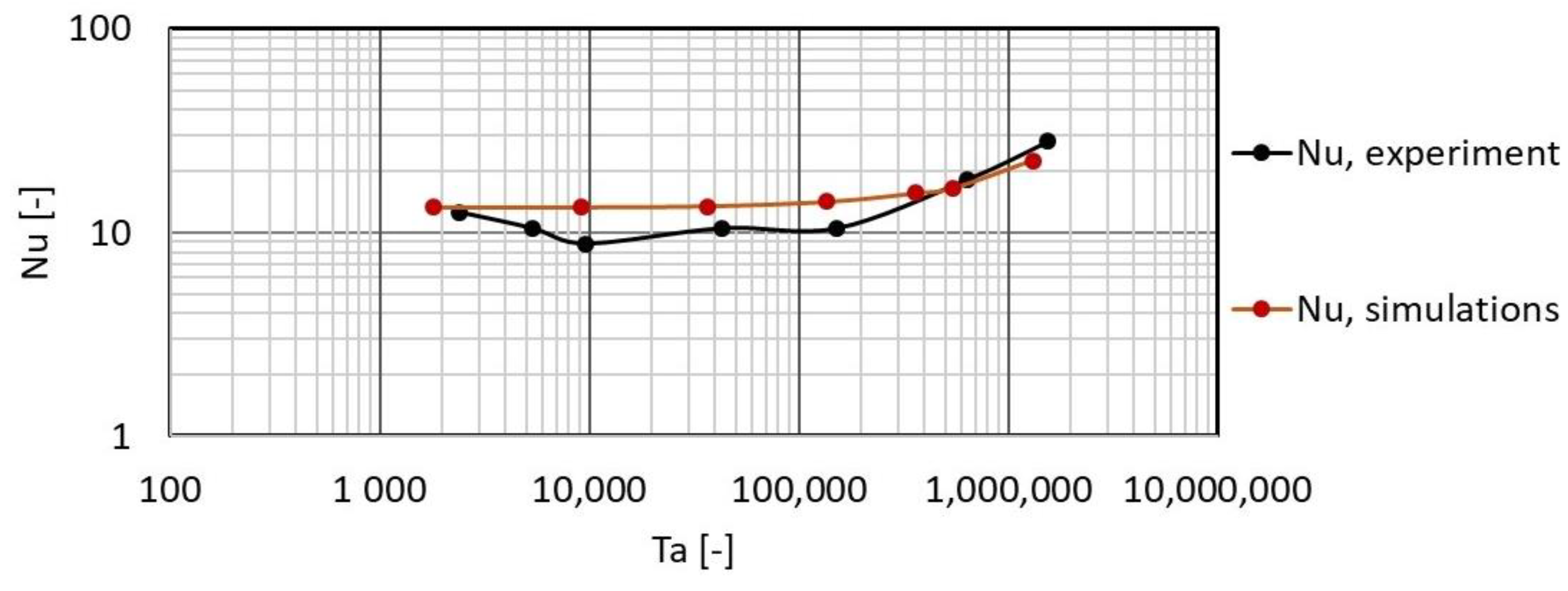
3.3. Local Heat Transfer Description in a Turbulent TCP Flow in a Grooved Air Gap

This final section presents the application of the workflow in configuring a grooved air gap which mimics the geometrical conditions inside an EM. The flow cases follow from the experiments performed in Bouafia [7], where local and global heat transfer results are presented for turbulent TCP flow in smooth and grooved air gaps.

3.3.1. Definition of Computational Domain and Boundary Conditions (Step 1)

The computational domain presents the test rig, shown in Figure 1 in Bouafia [7]. The exact geometry of the grooved air gap in it is defined following Figure 2A and Table 1 in the same publication. As the air gap features a relatively high number of grooves, N g = 48 , the defined initial domain span includes three grooves. These have a high groove height to width ratio, γ = 1.81 . The air gap also has a large aspect ratio, which makes it suitable for the local depiction of entrance region effects as well as evolution of the heat transfer along the air gap. The whole computational domain is graphically presented in Figure 17, while its dimensions and other geometrical parameters are listed in Table 8. The side volume includes, following the description in Bouafia [7], only the volume which affects the air-gap entry and exit conditions.
The observed flow conditions are all defined at R e a x = 17,000 , which is also the highest R e a x value in Bouafia [7]. In order to ensure this, the inlet boundary conditions impose a mass flux of 9.6 kg/m2s. Three T a values, T a = { 1000 ;   3.35 × 10 6 ; 13.1 × 10 6 } , are considered; these result in the corresponding rotating velocities Ω = { 2.7 ; 158.9 ; 314.2 } [ r a d s ] to be imposed on the rotor surfaces, while all other walls are considered stationary. It can be seen that the lowest T a value presents conditions where the effects of rotational velocity are negligible. Thermal boundary conditions include temperature of the air, which is set as 313 K at the domain inlet. The air is modelled as an ideal gas. The stator has a temperature of 298 K. The rotor surface in the air gap is heated with a constant heat flux of q = 5500   W / m 2 . This follows from the heat flux profiles reported in Figure 5 in Bouafia [7]. The outlet is defined as a pressure outlet with 1 bar static pressure.

3.3.2. Initial 3D CFD Model Definition and Mesh Independence Study (Steps 2 and 3)

The initial 3D CFD model is constructed using the same settings as applied in the initial model of the previous case, and is thus not presented here specifically. The applied meshing also follows the same approach, with the structured mesh being used in the air gap, while the outside volume is split into different subdomains.
The mesh independence study, performed as the third step of the workflow, is conducted while considering the most adverse conditions, presented with T a = 13.1 × 10 6 . Meshes with 5.6 to 25 million elements were applied in simulations of these conditions with the initial model. The mesh, presented with its applied sizing in Table 9, was found to be adequate.

3.3.3. Definition of the Adequate 3D CFD Models (Steps 4, 5 and 6)

Definition of the adequate 3D CFD models for the considered flow conditions is carried out in the same manner as presented in previous sections, applying the initial model with the initial and doubled domain spans. The initial model with the initial domain span was found to be adequate for all three considered flow conditions. The detailed presentation of results and analysis is thus omitted. The suitability of the initial 3D CFD model in all considered conditions is the consequence of the high R e a x value that results in the dominant impact of axial velocity on flow development.

3.3.4. Analysis of Final Results (Step 7)

The results were analyzed to obtain N u profiles along the rotor. These profiles are for all three flow conditions shown in Figure 18, along with the profiles obtained from experimental measurements. Their comparison shows that simulations manage to capture the trends observed in experiments. They capture the peak in the N u profiles at the air-gap entrance as well as the gradual drop in N u values along the air-gap length. This points to the crucial impacts of the entrance region in addition to the axial velocity on the local heat transfer in the observed air gap. Simulations also correctly report the highest N u values for the highest T a value. Additionally, simulations and experiments show that the N u profiles are very similar for the lower two T a values, while the profile at the highest T a value clearly differs from them.
While simulations correctly capture the trends in N u profiles, they do not match their amplitudes in the major part of the air gap. Extensive analysis was performed to determine the reasons. This led to an important finding: the 3D CFD models can, if defined adequately, offer additional explanation for experimentally obtained results. Observing the N u profiles, it can be noted that the experimental N u values rise considerably near the air-gap exit; meanwhile, results from simulations do not express this increase. The reason why this appears only in experimental results seems to be in the presence of heat losses across the rotor side surfaces, a fact which is mentioned in Bouafia [7]. These losses can also explain the drop in rotor surface temperature at the air-gap end, which can be noted in Figure 5 in Bouafia [7]. At the same time, a nearly constant heat flow to the rotor surface at R e a x = 17,000 is reported on the same figure in [7]. This drop in the rotor surface temperature along with nearly unchanged heat flow could lead to an increase in the experimentally reported α values, and hence in the reported N u values at the air-gap end also. And since the same effects are present at the air-gap entry, the high N u values there could also be explained with them. On the contrary, rotor surface temperature in simulations constantly increases from the entrance to the exit of the air gap, as rotor sides are considered adiabatic. This eliminates the possibility for an α increase close to the air-gap exit, and lowers α values at the air-gap entrance.
Due to this important difference between simulations and experiments, it can be claimed that the numerically obtained N u values are more accurate than what the graph in Figure 18 proposes. Thus, it can also be concluded that numerical results, though different from experiments, cannot be considered inaccurate. Furthermore, the additional and important benefit of defining adequate 3D CFD models is pointed out. With such models on hand, additional explanations for experimentally obtained results can be defined and used to improve experimental procedures.

4. Conclusions

The paper presents an innovative workflow for the construction of adequate 3D CFD models for thorough flow and heat transfer analysis in EM air gaps. The workflow is suitable for cases of various flow phenomena that appear in different air gaps exposed to different operating conditions. As such, the workflow also provides clarification to current state, where notable discrepancies exist between experimentally obtained results.
The workflow combines multiple contributions that enable the definition of adequate and computationally efficient 3D CFD models for certain flow conditions in an arbitrary EM air gap. First, it proposes a focus shift from the observation of specific and highly variable air-gap flow phenomena to the observation of their underlying flow characteristics. The vortex structures, flow unsteadiness and entrance region were defined as such. These characteristics can be readily detected with 3D CFD tools. In order to perform this detection, the workflow introduces the initial, specifically defined 3D CFD model that is a combination of settings, predicted as generally the most suitable. It then determines the adequately refined mesh for the flow conditions under consideration. The model and the adequately refined mesh represent the foundation for a reliable detection of the various underlying flow characteristics. This is followed through with step-by-step adaptations of the 3D CFD model, in order to ensure adequate modelling of the detected underlying flow characteristics. In the end, adequate 3D CFD models for the observed flow conditions in an air gap are obtained. These differ between different imposed conditions, leading to the application of the computationally most expensive models only in conditions that require them.
Validation of the workflow is presented with literature-based examples of different air gaps and flow conditions in them. These span from the laminar developed flow to turbulent flow, in which the entrance region determines heat transfer magnitude. Results show that the workflow meets the set requirements regarding detection of underlying flow characteristics, definition of the adequate 3D CFD models and the generation of valid and computationally efficient heat transfer descriptions. Results with the constructed models correspond well with experimentally obtained data for all considered flow cases. The provided discussions on the causes for changes in N u values with increases in T a number or along the air gap show that the models can deliver additional insights to experimentally obtained results. These insights can be used beneficially when designing experimental procedures. The confirmed ability of the workflow to determine conditions at which transient simulations are to be applied, as well as to optimize the computational domain span, provides further improvements over current means. The overall computational costs for the whole range of air-gap flow conditions can be decreased by an order of magnitude.
Combining the listed characteristics, the workflow introduces a reliable as well as computationally efficient tool for modelling the flow in a whole range of air-gap operating conditions. While the EM development process is increasingly relying on front-loading with virtual design, this proposed workflow provides a needed tool for improved systematic exploration of an EM design space. With it, reliable heat transfer correlations can be obtained for various air-gap flow conditions, which increases the chances of achieving right-first-time approaches in the design of EM cooling systems.

Author Contributions

Conceptualization, A.Ž. and T.K.; software, A.Ž.; validation, A.Ž.; formal analysis, A.Ž. and T.K.; data curation, A.Ž.; writing—original draft, A.Ž.; writing—review and editing, T.K.; visualization, A.Ž.; project administration, T.K.; funding acquisition, T.K. All authors have read and agreed to the published version of the manuscript.

Funding

This research was funded by the Slovenian Research Agency (research core funding No. P2-0401–Energy engineering) and the Slovenian Ministry of Education, Science and Sport through the program MOTZART.

Data Availability Statement

The data presented in this study are available on request from the corresponding authors.

Acknowledgments

The authors acknowledge the financial support from the Slovenian Research Agency (research core funding No. P2-0401–Energy engineering) and from the Slovenian Ministry of Education, Science and Sport through the programme MOTZART.

Conflicts of Interest

The authors declare no conflict of interest. The funders had no role in the design of the study, in the collection, analyses, or interpretation of data.

Nomenclature

acronyms/abbreviations
TCTaylor–Couette R radius [m]
TCPTaylor–Couette–Poiseuille L air-gap length [m]
EMelectric machine b groove height [m]
PIVparticle image velocimetry c groove width [m]
LDVlaser Doppler velocimetry N g number of grooves [-]
IRinfrared S m reference heat transfer area [m2]
RANSReynolds averaged Navier–Stokes R m mean radius [m]
LESlarge eddy simulations o air-gap wetted perimeter [m]
DNSdirect numerical simulations D h hydraulic diameter [m]
dimensionless numbers u average velocity [m/s]
N u Nusselt number p pressure [Pa]
η ratio of air-gap rotor and stator radii A air-gap cross sectional area [m2]
Γ air-gap axial aspect ratio B equivalent gap height [m]
γ groove aspect ratio B = A / ( 2 π R 1 )
R e Reynolds number T temperature [K]
T a Taylor number Q ˙ heat flow [W/m2]
F g geometric factor q ˙ heat flux [W/m2s]
P geometric factor ν kinematic viscosity [m2/s]
f friction factor μ dynamic viscosity [Pa∙s]
y + non-dimensional distance from the wall Ω rotational velocity [rad/s]
CCourant number ρ density [kg/m3]
indexes λ thermal conductivity [W/mK]
1rotor α convective heat transfer coefficient
2stator [W/m2K]
axaxial t time [s]
τ tangential v velocity vector [m/s]
effeffective I unit tensor [-]
bbulk e 0 total energy [m2/s2]
crcritical k turbulence kinetic energy [m2/s2]
Tturbulent ω specific dissipation rate [1/s]
variables Γ k effective   diffusivity   of   k [Pa∙s]
Γ ω effective   diffusivity   of   ω [Pa∙s] Y k dissipation   of   k [kg/m∙s3]
G k ˜ generation   of   k [kg/m∙s3] Y ω dissipation   of   ω [kg/m3∙s2]
G ω generation   of   ω [kg/m3∙s2] D ω cross-diffusion term [kg/m3∙s2]

References

  1. Couette, M. Oscillations tournantes d’un solide de révolution en contact avec un fluide visqueux. C. R. Séances L’acad. Sci. Paris 1887, 105, 1064–1067. [Google Scholar]
  2. Taylor, G.I. Stability of viscous liquid contained between two rotating cylinders. Philos. Trans. R. Soc. Lond. Ser. A 1923, 223, 289–343. [Google Scholar]
  3. Hamidi, K.; Rezoug, T.; Poncet, S. Numerical modeling of heat transfer in Taylor-Couette-Poiseuille systems. Defect Diffus. Forum 2019, 390, 125–132. [Google Scholar] [CrossRef]
  4. Kaye, J.; Elgar, E.C. Modes of adiabatic and diabatic fluid flow in an annulus with an inner rotating cylinder. Trans. ASME 1958, 80, 753–765. [Google Scholar] [CrossRef]
  5. Gardiner, S.R.M.; Sabersky, R.H. Heat transfer in an annular gap. Int. J. Heat Mass Transf. 1978, 21, 1459–1466. [Google Scholar] [CrossRef]
  6. Lee, Y.N.; Minkowycz, W.J. Heat transfer characteristics of the annulus of twocoaxial cylinders with one cylinder rotating. Int. J. Heat Mass. Transf. 1989, 32, 711–722. [Google Scholar] [CrossRef]
  7. Bouafia, M.; Bertin, Y.; Saulnier, J.B. Experimental analysis of heat transfer in a narrow and grooved annular gap with rotating inner cylinder. Int. J. Heat Mass. Transf. 1998, 41, 1279–1291. [Google Scholar] [CrossRef]
  8. Fénot, M.; Dorignac, E.; Giret, A.; Lalizel, G. Convective heat transfer in the entry region of an annular channel with slotted rotating inner cylinder. Appl. Therm. Eng. 2013, 54, 345–358. [Google Scholar] [CrossRef]
  9. Liu, D.; Kang, I.S.; Cha, J.E.; Kim, H.B. Experimental study on radial temperature gradient effect of a Taylor-Couette flow with axial wall slits. Exp. Therm. Fluid Sci. 2011, 35, 1282–1292. [Google Scholar] [CrossRef]
  10. Aubert, A.; Poncet, S.; Le Gal, P.; Viazzo, S.; Le Bars, M. Velocity and temperature measurements in a turbulent water-filled Taylor-Couette-Poiseuille system. Int. J. Therm. Sci. 2015, 90, 238–247. [Google Scholar] [CrossRef]
  11. Fénot, M.; Bertin, Y.; Dorignac, E.; Lalizel, G. A review of heat transfer between concentric rotating cylinders with or without axial flow. Int. J. Therm. Sci. 2011, 50, 1138–1155. [Google Scholar] [CrossRef]
  12. Nouri-Borujerdi, A.; Nakhchi, M.E. Heat transfer enhancement in annular flow with outer grooved cylinder and rotating inner cylinder: Review and experiments. Appl. Therm. Eng. 2017, 120, 257–268. [Google Scholar] [CrossRef]
  13. Nouri-Borujerdi, A.; Nakhchi, M.E. Optimization of the heat transfer coefficient and pressure drop of Taylor-Couette-Poiseuille flows between an inner rotating cylinder and an outer grooved stationary cylinder. Int. J. Heat Mass. Transf. 2017, 108, 1449–1459. [Google Scholar] [CrossRef]
  14. Dirker, J.; Van Der Vyver, H.; Meyer, J.P. Convection heat transfer in concentric annuli. Exp. Heat Transf. 2004, 17, 19–29. [Google Scholar] [CrossRef]
  15. Mehrez, I.; Gheith, R.; Aloui, F.; Ben Nasrallah, S. Theoretical and numerical study of Couette-Taylor flow with an axial flow using lattice Boltzmann method. Int. J. Numer. Methods Fluids 2019, 90, 427–441. [Google Scholar] [CrossRef]
  16. Afra, B.; Amiri Delouei, A.; Mostafavi, M.; Tarokh, A. Fluid-structure interaction for the flexible filament’s propulsion hanging in the free stream. J. Mol. Liq. 2021, 323, 114941. [Google Scholar] [CrossRef]
  17. Jalali, A.; Delouei, A.A.; Khorashadizadeh, M.; Golmohamadi, A.; Karimnejad, S. Mesoscopic simulation of forced convective heat transfer of Carreau-Yasuda fluid flow over an inclined square: Temperature-dependent viscosity. J. Appl. Comput. Mech. 2020, 6, 307–319. [Google Scholar] [CrossRef]
  18. Hayase, T.; Humphrey, J.A.C.; Greif, R. Numerical calculation of convective heat transfer between rotating coaxial cylinders with periodically embedded cavities. J. Heat Transf. 1992, 114, 589–597. [Google Scholar] [CrossRef]
  19. Bouafia, M.; Ziouchi, A.; Bertin, Y.; Saulnier, J.B. Experimental and numerical study of heat transfer in an annular gap without axial flow with a rotating inner cylinder. Int. J. Therm. Sci. 1999, 38, 547–559. [Google Scholar] [CrossRef]
  20. Sommerer, Y.; Lauriat, G. Numerical study of steady forced convection in a grooved annulus using a design of experiments. J. Heat Transf. 2001, 123, 837–848. [Google Scholar] [CrossRef]
  21. Hwang, J.Y.; Yang, K.S. Numerical study of Taylor-Couette flow with an axial flow. Comput. Fluids 2004, 33, 97–118. [Google Scholar] [CrossRef]
  22. Poncet, S.; Haddadi, S.; Viazzo, S. Numerical modeling of fluid flow and heat transfer in a narrow Taylor-Couette-Poiseuille system. Int. J. Heat Fluid Flow 2011, 32, 128–144. [Google Scholar] [CrossRef] [Green Version]
  23. Poncet, S.; Da Soghe, R.; Bianchini, C.; Viazzo, S.; Aubert, A. Turbulent Couette-Taylor flows with endwall effects: A numerical benchmark. Int. J. Heat Fluid Flow 2013, 44, 229–238. [Google Scholar] [CrossRef] [Green Version]
  24. Foudrinier, M.; Poncet, S.; Moreau, S.; Torriano, F. Numerical study in a Taylor-Couette-Poiseuille system. In Proceedings of the 24th Annual Conference of the CFD Society of Canada, Kelowna, BC, Canada, 26–29 June 2016. [Google Scholar]
  25. Romanazzi, P.; Howey, D.A. Air-gap convection in a switched reluctance machine. In Proceedings of the 2015 Tenth International Conference on Ecological Vehicles and Renewable Energies, EVER 2015, Monte Carlo, Monaco, 31 March–2 April 2015. [Google Scholar] [CrossRef] [Green Version]
  26. Lancial, N.; Torriano, F.; Beaubert, F.; Harmand, S.; Rolland, G. Study of a Taylor-Couette-Poiseuille flow in an annular channel with a slotted rotor. In Proceedings of the 2014 International Conference on Electrical Machines (ICEM 2014), Berlin, Germany, 2–5 September 2014; pp. 1422–1429. [Google Scholar] [CrossRef]
  27. Lancial, N.; Torriano, F.; Beaubert, F.; Harmand, S.; Rolland, G. Taylor-Couette-Poiseuille flow and heat transfer in an annular channel with a slotted rotor. Int. J. Therm. Sci. 2017, 112, 92–103. [Google Scholar] [CrossRef]
  28. Nouri-Borujerdi, A.; Nakhchi, M.E. Prediction of local shear stress and heat transfer between internal rotating cylinder and longitudinal cavities on stationary cylinder with various shapes. Int. J. Therm. Sci. 2019, 138, 512–520. [Google Scholar] [CrossRef]
  29. Wereley, S.T.; Lueptow, R.M. Spatio-temporal character of non-wavy and wavy Taylor-Couette flow. J. Fluid Mech. 1998, 364, 59–80. [Google Scholar] [CrossRef] [Green Version]
  30. Wereley, S.T.; Lueptow, R.M. Velocity field for Taylor–Couette flow with an axial flow. Phys. Fluids 1999, 11, 3637. [Google Scholar] [CrossRef] [Green Version]
  31. Lueptow, R.M.; Docter, A.; Min, K. Stability of axial flow in an annulus with a rotating inner cylinder. Phys. Fluids A 1992, 4, 2446–2455. [Google Scholar] [CrossRef] [Green Version]
  32. Dong, Y.; Yan, Y.; Liu, C. New visualization method for vortex structure in turbulence by lambda2 and vortex filaments. Appl. Math. Model. 2016, 40, 500–509. [Google Scholar] [CrossRef]
  33. Ansys®, Academic Research Workbench, Release 19.2., Help System, Workbench User’s Guide, ANSYS, Inc.
  34. Ansys®, Academic Research Fluent, Release 19.2., Help System, Fluent Theory Guide, ANSYS, Inc.
  35. Munters, W.; Meneveau, C.; Meyers, J. Shifted periodic boundary conditions for simulations of wall-bounded turbulent flows. Phys. Fluids 2016, 28, 025112. [Google Scholar] [CrossRef] [Green Version]
  36. Versteeg, H.K.; Malalasekera, W. An Introduction to Computational Fluid Dynamics: The Finite Volume Method; [OpenFOAM]; Longman Scientific & Technical: Harlow, UK; Wiley: New York, NY, USA, 2015. [Google Scholar]
  37. Menter, F.R.; Langtry, R.; Völker, S. Transition Modelling for General Purpose CFD Codes. Flow Turbul. Combust. 2006, 77, 277–303. [Google Scholar] [CrossRef]
Figure 1. Appearance of the four main flow modes according to the axial and rotational velocity magnitudes in an air gap (left) and the basic form of Taylor vortices (right).
Fluids 07 00273 g001
Figure 2. Presentation of the air-gap defining dimensions.
Fluids 07 00273 g002
Figure 3. Schematic presentation of the workflow that was devised to obtain adequate 3D CFD models for air-gap flow simulations.
Fluids 07 00273 g003
Figure 4. An example of an EM geometry (top left) from which the air gap and its surrounding volume are extracted (top right) to define the computational domain as well as its apparent boundary conditions (bottom).
Fluids 07 00273 g004
Figure 5. Comparison of results from TCP flow simulations in a smooth air gap that represent the impact of the computational domain span on flow development. The iso-surfaces with a λ 2 value of 1500 1/s2 are depicted on the left, and average velocity vectors near the rotor surface are shown on the right.
Fluids 07 00273 g005
Figure 6. Air gap (solid) and outside volume (transparent) geometry as used in the basic numerical model of flow with wavy Taylor vortices. The applied boundary conditions are also depicted.
Fluids 07 00273 g006
Figure 7. Average axial and tangential velocities in three points along the air gap (left) and wall shear stresses on the rotor and stator (right), resulting from the mesh independence study.
Fluids 07 00273 g007
Figure 8. Axial velocity evolution at six points (locations indicated in the legend) after converged state is achieved in simulations with the initial model featuring initial domain span.
Fluids 07 00273 g008
Figure 9. Relative standard deviations of axial and tangential velocities at six points along the air gap in the cases of the basic and doubled domains.
Fluids 07 00273 g009
Figure 10. Iso-surfaces with a λ 2 value of −0.2 1/s2 in simulations with the initial and doubled domain spans.
Fluids 07 00273 g010
Figure 11. Depiction of Taylor vortices in simulations, performed following the workflow (left), and from the results of Hwang [18] (right). The vortices in performed simulations are depicted with contours of velocity magnitude at mid-radial height.
Fluids 07 00273 g011
Figure 12. Air gap (solid) and outside volume (transparent) geometry as used in the initial model of a smooth air gap in Lee [6]. The applied boundary conditions are also depicted.
Fluids 07 00273 g012
Figure 13. Average axial velocities at three points, along with the air gap and rotor shear stress results used in the mesh independence study. The points are located 20, 40 and 60 mm from air-gap entry.
Fluids 07 00273 g013
Figure 14. Iso-surfaces with a λ 2 value of 60 1/s2 from simulations at the lowest T a value, viewed from the bottom (top left) and top (top right), and viscosity ratio values in the air-gap cross section (bottom).
Fluids 07 00273 g014
Figure 15. Comparison of N u values obtained from simulations at different T a numbers with N u values from experimental measurements presented in Lee [6].
Fluids 07 00273 g015
Figure 16. Top view of λ 2 iso-surfaces inside the air gap obtained from simulations of the three different flow cases from Lee [6].
Fluids 07 00273 g016
Figure 17. Air gap and outside volume geometry as used in the initial numerical model of the grooved air gap from Bouafia [7]. The applied boundary conditions are also depicted.
Fluids 07 00273 g017
Figure 18. Simulated and experimentally obtained N u profiles on the rotor along the length of the air gap for three different T a values.
Fluids 07 00273 g018
Table 1. Dimensions and geometrical parameters of the air gap in which wavy Taylor vortices are observed.
Dimension R 1
[mm]
R 2
[mm]
e
[mm]
D h
[mm]
L
[mm]
L i n
[mm]
L o u t
[mm]
η
[-]
Γ
[-]
value43.452.38.917.841020500.8346.07
Table 2. Flow parameters for which wavy Taylor vortices are observed.
Flow Parameter R e a x
[-]
T a
[-]
u
[m/s]
Ω
[rad/s]
value9.834500.00835.4
Table 3. Adequate mesh sizing properties.
Mesh PropertyCell Axial
Size
[mm]
Cell Radial and
Azimuth Size
[mm]
Inflation
Thickness
[mm]
Number of
Inflation Layers
[-]
Cell Count
[106]
value0.750.75282.7
Table 4. Dimensions and geometrical parameters of the smooth air gap from Lee [6].
Dimension R 1
[mm]
R 2
[mm]
R 3
[mm]
R 4
[mm]
D h
[mm]
L
[mm]
L i n
[mm]
L o u t
[mm]
η
[-]
Γ
[-]
value55.5563.5253115.977.940160.8759.87
Table 5. Taylor numbers of considered flow cases from Lee [6].
Flow Case1234567
T a 1820914036,560137,000364,100546,3001,312,300
Table 6. The suitably refined mesh for considered flow conditions from Lee [6].
Mesh PropertyAverage Cell
Axial Size
[mm]
Cell Radial and
Azimuth Size
[mm]
Inflation
Thickness
[mm]
Number of
Inflation Layers
[-]
Cell Count
[106]
value0.50.31.5103.98
Table 7. Defined adequate numerical set-ups for the considered flow cases from Lee [6].
Flow Case1234567
steady/transientsteadysteadysteadysteadytransienttransienttransient
time step and
C value
////0.2 ms
2.4
0.2 ms
2.8
0.1 ms
2.12
domain span60°60°60°60°120°120°120°
turbulence model k ω SST
Table 8. Dimensions and geometrical parameters of the considered grooved air gap from Bouafia [7].
Dimension R 1
[mm]
R 2
[mm]
R 3
[mm]
R 4
[mm]
c
[mm]
b
[mm]
L
[mm]
L i n = L o u t
[mm]
g
[mm]
η
[-]
Γ
[-]
value1401451201308.31560458400.966120.8
Table 9. The suitably refined mesh for air gaps from Bouafia [7].
Mesh PropertyCell Axial
Size
[mm]
Cell Radial and
Azimuth Size
[mm]
Inflation
Thickness
[mm]
Number of
Inflation Layers
[-]
Cell Count
[106]
value0.80.4215 (stator)
20 (rotor)
23.1
Publisher’s Note: MDPI stays neutral with regard to jurisdictional claims in published maps and institutional affiliations.

