The Effects of Compressibility on the Performance and Modal Structures of a Sweeping Jet Emitted from Various Scales of a Fluidic Oscillator

Abstract

Investigations of fluidic oscillators, or sweeping jet actuators, have primarily been conducted within the incompressible flow regime, which limits the accuracy of estimating fluidic oscillator performance for compressible flows. The objective of this study was to evaluate the effects of gas compressibility on the performance of a fluidic oscillator. A commonly used fluidic oscillator geometry (the Bray geometry) was scaled to five different sizes, 3D printed, and tested over a range of air flow rates. High-speed Schlieren images captured the sweeping jet exiting the fluidic oscillators, and custom MATLAB algorithms were used to calculate the oscillation frequencies and angles. A spectral proper orthogonal decomposition (SPOD) method was used to identify and compare the mode structures within the flow fields. All the results were compared using dimensionless parameters to observe performance trends. The results showed that the oscillation frequencies were directly proportional to the flow rate, while the oscillation angles were inversely proportional to the flow rate, regardless of scale size. The angular velocities were not proportional to the flow rate or scale size and exhibited maxima within the evaluated ranges. For all scale sizes, the mode structures were symmetric across the centerlines of the fluidic oscillators and extended further beyond the fluidic oscillators at higher flow rates. These results enable the prediction of fluidic oscillator performance, which can significantly improve the design process for an application where a fluidic oscillator may be used, such as aerospace applications, power generation, heat exchangers, or medical devices.

1. Introduction

Fluidic oscillators, or sweeping jet actuators, are channel geometries that convert steady, fully developed flows from their inlets into unsteady turbulent flows at their outlets. The outlet flow of a fluidic oscillator is typically in the form of a jet that continuously sweeps back and forth. A fluidic oscillator has two primary internal geometries: a main mixing chamber and a set of feedback channels, as shown in Figure 1. The unsteady flow that is created by the fluidic oscillator is a result of the Coandă effect, which causes the incoming fluid to adhere to one side of the mixing chamber (shown at (Φ = 0° and 180° in Figure 1) [1]. The adhered flow eventually begins to separate from the wall of the mixing chamber, which creates a vortex of recirculating flow in the mixing chamber. This vortex then grows larger and eventually diverts the incoming flow towards the opposite side of the mixing chamber (Φ = 90° and 270° in Figure 1), where it adheres to the wall and starts the vortex-generation cycle again. The oscillating flow within the main chamber is amplified by the feedback channels, which assist in diverting the incoming flow to alternating sides of the mixing chamber. The internally diverted flow then exits through the nozzle at a range of angles corresponding to the available flow path.

Owing to their ability to produce flow with high turbulent kinetic energy, fluidic oscillators have been used in a variety of applications such as shower heads, convective heat transfer equipment, aircraft wings, and turbine blades [2,3,4,5]. Recent fluidic oscillator research has been primarily focused on using the sweeping jet as a means of flow control, where the oscillator is positioned in a manner that disrupts the boundary layer of a fluid moving over a surface [3,6,7]. Koklu demonstrated a significant delay in boundary layer separation over the NASA hump model after the implementation of an array of fluidic oscillators [8]. Multiple groups have also demonstrated that placing fluidic oscillators near the leading edge of an airfoil has the potential to delay boundary layer separation, which can ultimately increase lift and decrease drag on the airfoil [4,7,9,10,11]. With regards to the airfoil-shaped blades in turbines, Hossain et al. demonstrated that using sweeping jets for film cooling improved the overall cooling performance of a transonic turbine cascade [5].

Despite the increased use of fluidic oscillators in applications within transonic (or even supersonic) flow regimes, there exist limited data related to the effects that fluid compressibility has on a fluidic oscillator’s performance. Additionally, there is limited research on those effects across different scales of the same fluidic oscillator design. Existing research on this topic includes work from Portillo et al., who observed an increase in the oscillation frequency, and a decrease in the oscillation angle, as the flow rate through the oscillator increased and the scale of the fluidic oscillator decreased; however, that research did not compare these results non-dimensionally across scales [12]. Other research on this topic includes work from both von Gosen et al. (experimental) and Oz and Kara (computational), who observed similar results for a single fluidic oscillator—specifically, a plateau in the oscillation frequency as the flow approached choked conditions [13,14]. While Park et al. characterized a fluidic oscillator that produced supersonic flow at its outlet, that work only demonstrated results that were correlated to dimensions of single geometric features within a fluidic oscillator [15].

Given this gap in the current literature, the objective of this study was to evaluate the effects of compressibility on the performance of a sweeping jet produced by a fluidic oscillator across various flow rates and scales. The performance of the sweeping jet was characterized by the oscillation frequency, oscillation angle, angular velocity, and modal structures. Those performance metrics were evaluated using high-speed Schlieren images and pressure probes, which provided information about the sweeping jet’s position over time. It was observed that the oscillation frequency, oscillation angle, and angular velocity of the sweeping jet were correlated to the Mach number at the exit throat, regardless of the fluidic oscillator size. It was also observed that the mode structures at harmonic frequencies of the oscillation frequencies were similar across flow rates and fluidic oscillator sizes.

2. Materials and Methods

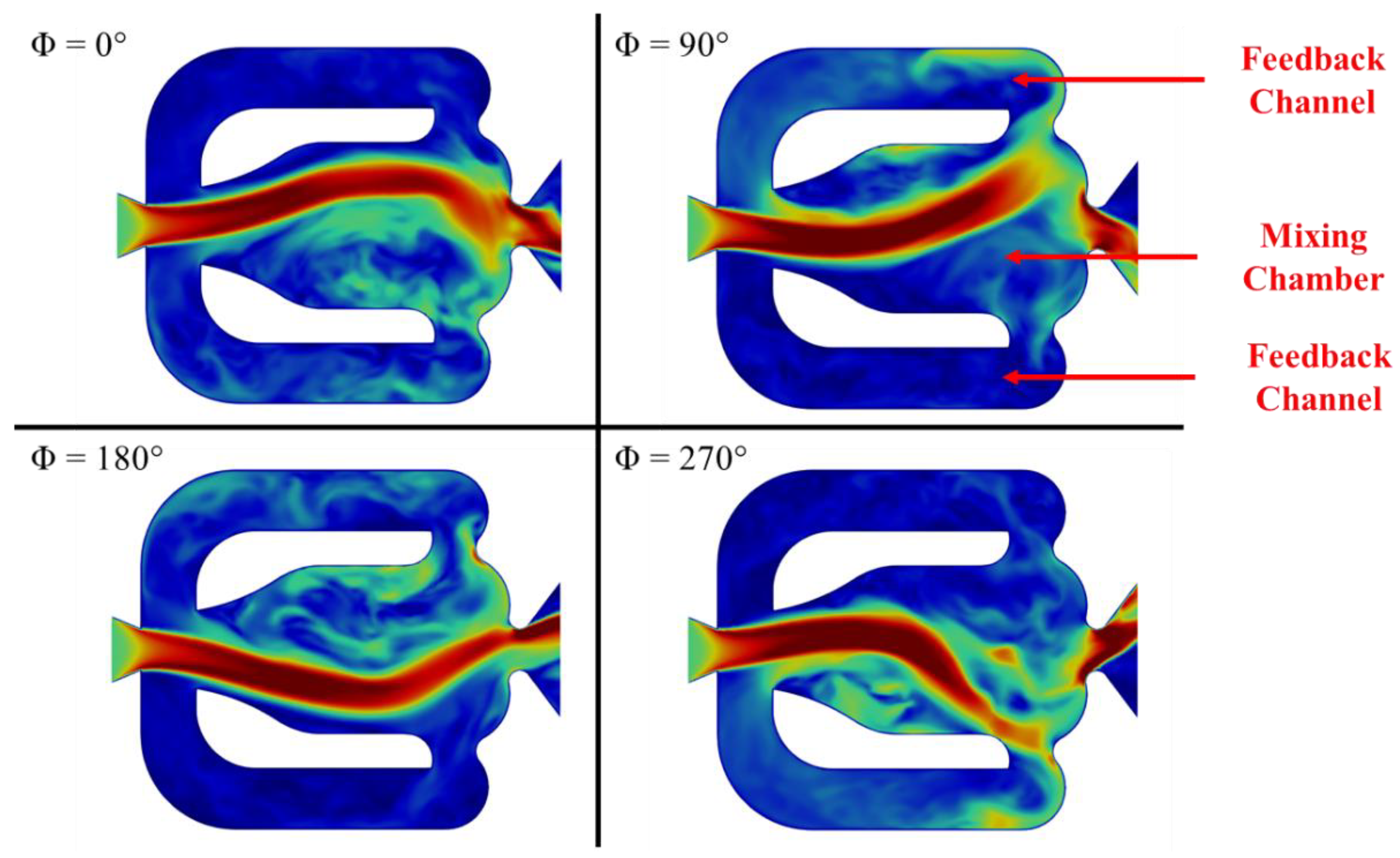
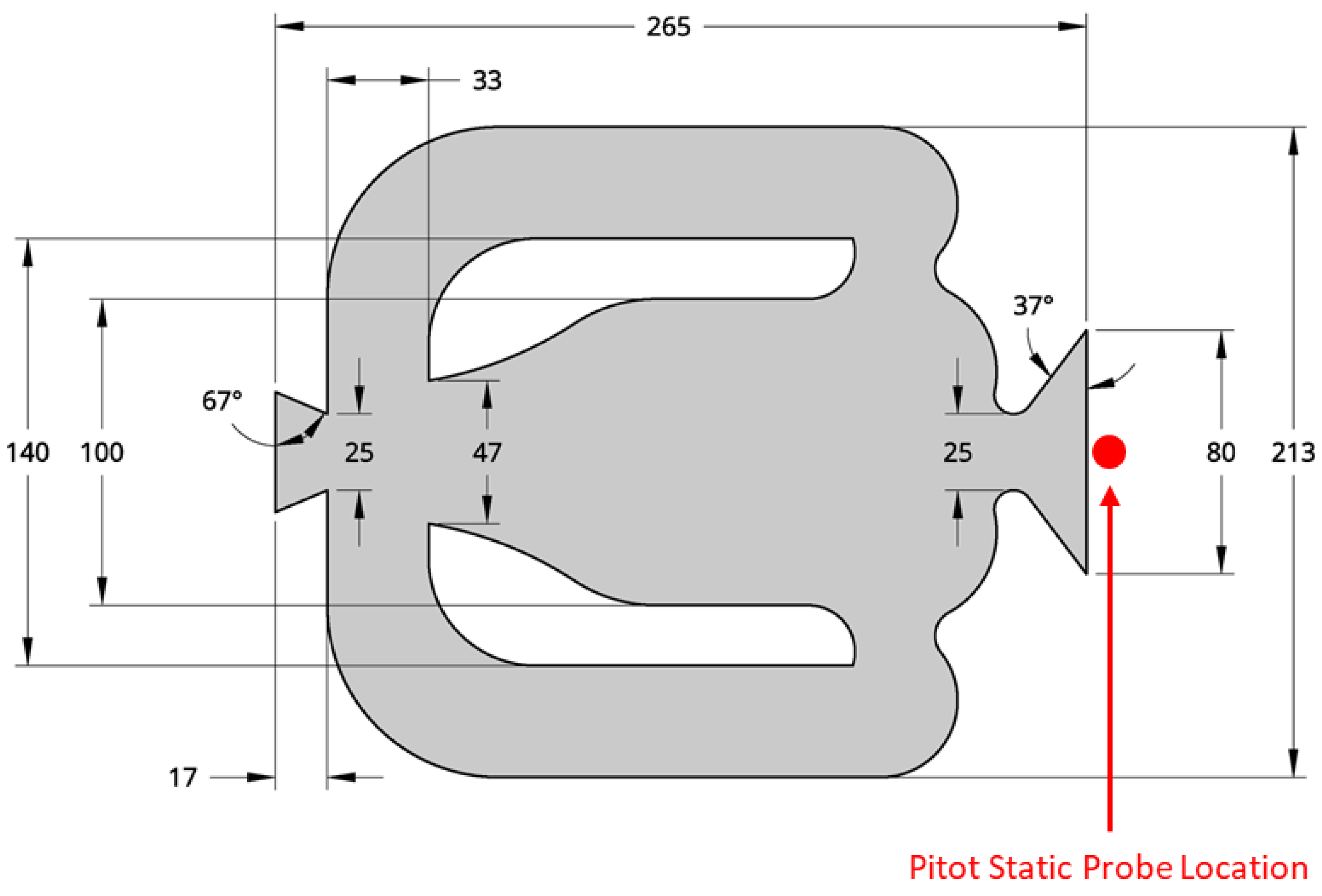
2.1. Fluidic Oscillators and Flow Parameters

The fluidic oscillators that were used in this study were based on the baseline fluidic oscillator geometry that was specified by Portillo et al., which was derived from Bray [12,16]. That geometry, detailed in Figure 2, was scaled to five different size ratios and additively manufactured using a stereolithography method (Clear Resin, Form 2, Formlabs, Somerville, MA, USA). The scale models were reduced in size by ratios of 1:2, 1:4, 1:6, 1:8, and 1:10, which resulted in exit throat widths of 12.5, 6.25, 4.15, 3.13, and 2.5 mm, respectively.

Each of these fluidic oscillator geometries had a thickness that was equal to the width of their exit throat (w_t), which resulted in exit throats that had square cross-sectional areas. The hydraulic diameters (D_h) of the exit throats were calculated using

$$D_h=\frac{4A_c}{Perim}=\frac{4\left(w_t\ast w_t\right)}{w_t+w_t+w_t+w_t}=\frac{4{w_t}^2}{4w_t}=w_t,$$

(1)

which depended on the relationship between the cross-sectional area (A_c) and perimeter (Perim) of the exit throat. Since the exit throats had square cross-sectional areas, the derivation shown in Equation (1) shows the equivalence of D_h to w_t. To simplify the connection of tubing for gas delivery, each fluidic oscillator was fabricated with barbed fittings that had an inner cross-sectional area that was equal to the size of the beginning of the entrance nozzle.

All the scales of the fluidic oscillators were exposed to a range of air flow rates, which were supplied by a compressed air source and controlled by a pressure regulator (1042-Z21957, Fairchild).

Table 1. Test matrix showing air inlet pressure ranges for fluidic oscillators.

Scale	Air Inlet Pressure Range
1:2	115–184 kPa
1:4	115–225 kPa
1:6	115–308 kPa
1:8	115–308 kPa
1:10	115–308 kPa

illustrates the test matrix for different combinations of fluidic oscillator scales and air inlet pressures, which ranged from 115 to 308 kPa (2–30 psig). The highest air pressures that were achieved for the 1:2 and 1:4 scales were 184 and 225 kPa (12 and 18 psig), respectively; the compressed air source did not supply the flow rates that were needed to attain higher inlet pressures at those scales. The flow velocity exiting the fluidic oscillator was measured at the exit of the fluidic oscillator (in the center of the diverging nozzle) with a pitot static probe; the location of that probe can be seen in Figure 2. The pitot static probe was fabricated out of two hypodermic needles, a method that had previously been used by Melton et al. [4]. The hypodermic needle that was responsible for measuring the stagnation, or total, pressure was modified to feature a blunt tip (instead of a bevel), and the shaft was positioned parallel to the centerline of the fluidic oscillator. The hypodermic needle that was responsible for measuring the static pressure was parallelly fastened to the first needle, its lumen was crimped shut, and a hole was machined through the side of the shaft (perpendicular to the centerline of the fluidic oscillator).

A custom virtual instrument (VI) was created in LabVIEW (LabVIEW 2019, National Instruments, Austin, TX, USA) to read and log data from two pressure transducers (PX309-030G5V, Omega Engineering, Inc., Norwalk, CT, USA), which measured the absolute static and stagnation pressure from the hypodermic needle probes at a sampling rate of 10 kHz. The Mach number (M) was calculated with

$$M=\sqrt{\frac{2}{\gamma -1}\left({\left(\frac{P_o}{P}\right)}^{\frac{\gamma -1}{\gamma }}-1\right)},$$

(2)

and depended on the static pressure (P), stagnation pressure (P_o), and ratio of specific heats for air (γ, 1.4). The air was assumed to be an ideal gas and the static density of the air (ρ) was calculated using

$$\rho =\frac{P{M}_w}{RT},$$

(3)

which took into account P, the molecular weight of air (M_w, 0.029 kg·mol⁻¹); the universal gas constant (R, 8.314 J·mol⁻¹·K⁻¹); and the ambient temperature of the air (T, 294 K). The temperature of the air was measured with a thermal camera (TG130, Teledyne FLIR LLC, Wilsonville, OR, USA), which had an accuracy of ±4 K. The velocity of the air (v) was calculated with

$$v=M\sqrt{\frac{\gamma RT}{M_w}},$$

(4)

since M, γ, R, T, and M_w were known or had been calculated. The relationship that was used to calculate the Reynolds number (Re),

$$Re=\frac{\rho v{D}_h}{\mu },$$

(5)

depended on ρ, v, D_h, and the dynamic viscosity of the air (µ, 1.846 × 10⁻⁵ N·s·m⁻²). A custom MATLAB (MATLAB R2020a, The MathWorks, Inc., Natick, MA, USA) script was written to process the data that were recorded with the pitot static probe. The propagation of uncertainty from the pressure transducers was calculated for M, ρ, v, and Re using the following equations:

$$\delta M=\sqrt{{\left(\frac{\partial M}{\partial P_o}\delta P_o\right)}^2+{\left(\frac{\partial M}{\partial P}\delta P\right)}^2}$$

(6)

$$\delta \rho =\sqrt{{\left(\frac{\partial \rho }{\partial P}\delta P\right)}^2+{\left(\frac{\partial \rho }{\partial T}\delta T\right)}^2}$$

(7)

$$\delta v=\sqrt{{\left(\frac{\partial v}{\partial M}\delta M\right)}^2+{\left(\frac{\partial v}{\partial T}\delta T\right)}^2}$$

(8)

$$\delta Re=\sqrt{{\left(\frac{\partial Re}{\partial \rho }\delta \rho \right)}^2+{\left(\frac{\partial Re}{\partial v}\delta v\right)}^2}$$

(9)

The uncertainty of M (δM) depended on the uncertainty of P and P_o (δP and δP_o, respectively), which were represented by the standard deviation of the collected data. The uncertainty of ρ (δρ) only depended on δP and the uncertainty of v (δv) depended only on δM, which was determined using Equation (6). Both δρ and δv were then used to calculate the uncertainty of Re (δRe).

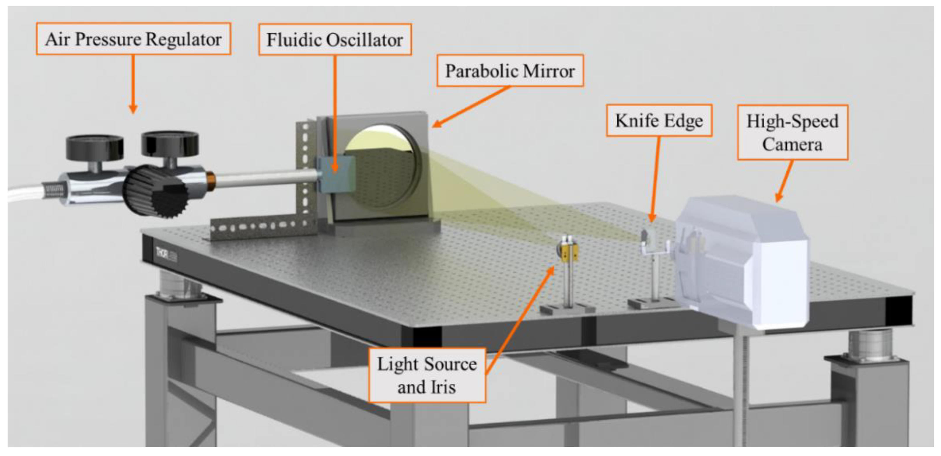
2.2. Schlieren Imaging Setup

Schlieren images take advantage of the refraction of collimated light that is caused by density gradients in the flow field, which provides the ability to visualize flow structures that are normally invisible to the naked eye [17]. As demonstrated by previous groups, Schlieren images provide a method for evaluating the performance of fluidic oscillators [12,13,18,19]. The Schlieren imaging setup in this study used a 1 mm diameter iris to focus a 2.7 W light source (CBT-140-W, Luminus, Sunnyvale, CA, USA) onto a 152.4 mm parabolic mirror (focal length of 1.524 m). A rendering of the experimental setup is shown in Figure 3, which also depicts the reflection of the light from the parabolic mirror onto a high-speed camera (Photron FASTCAM SA-Z, Photron, Tokyo, Japan). A knife edge was placed at the focal point of the light before it reached the camera, which spatially filtered the image being captured and created localized bright and dark regions that represented changes in the first derivative of the index of refraction (and thus changes in local density gradient). The images were recorded with the Photron FASTCAM Viewer Software (Version 4.0, Photron) and processed using custom MATLAB scripts to calculate the sweeping jet oscillation frequencies, oscillation angles, and mode structures. The MATLAB scripts are explained in more detail in the following sections.

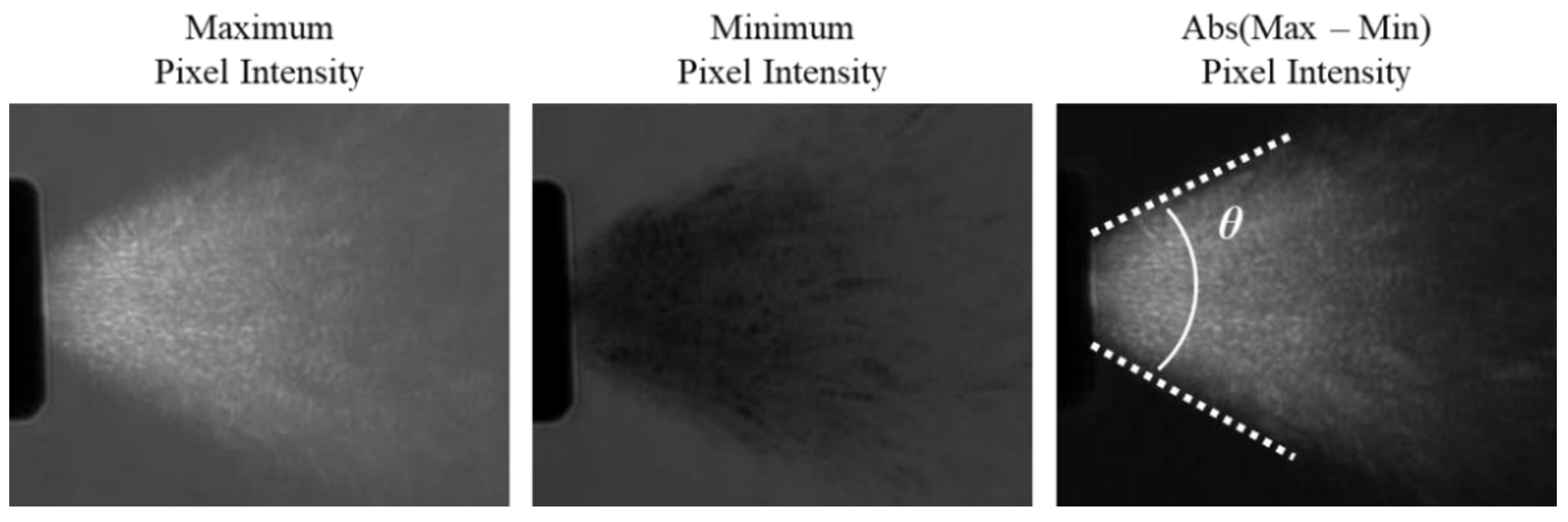
2.3. Oscillation Frequency, Oscillation Angle, and Jet Velocity Analysis

A total of 10,000 Schlieren images (512 × 1024 pixels) were recorded at 40 kHz for each of the five trials at each combination of flow rate and fluidic oscillator scale. Custom MATLAB scripts were developed to determine the oscillation frequency and oscillation angles of the fluidic oscillators from the Schlieren images. To calculate the oscillation frequency (f_osc), the average pixel intensity within a small window (located beside the center axis of the fluidic oscillator) of each image was recorded and plotted versus time. Then, a Fast Fourier Transform (FFT) was conducted using that data to determine the frequency at which the jet swept in and out of the evaluation window.

To calculate the oscillation angle (θ), the minimum and maximum pixel intensity for each pixel over the entire image set was recorded, and the difference between those two images produced a profile of where the flow had been during the trial. Figure 4 illustrates an example of the maximum and minimum pixel intensities across an image set, as well as the absolute difference between those images. The angle of that profile was measured using the angle tool in ImageJ (National Institutes of Health, Bethesda, MD, USA) and the standard deviation of the measured angle was calculated across the five image sets that were recorded at each fluidic oscillator scale and flow rate.

The oscillation frequency was represented with the dimensionless Strouhal number (St), which was calculated using

$$St=\frac{f_{osc}{D}_h}{v}.$$

(10)

The uncertainty of St (δSt) was calculated using

$$\delta St=\sqrt{{\left(\frac{\partial St}{\partial f_{osc}}\delta f_{osc}\right)}^2+{\left(\frac{\partial St}{\partial v}\delta v\right)}^2},$$

(11)

where the uncertainty of the oscillation frequency (δf_osc) represented the standard deviation of the data that were collected (n = 5), and δv was determined using Equation (8). The angular velocity (ω) of the jet and the uncertainty of the angular velocity (δω) were calculated using

$$\omega =\frac{f_{osc}\theta \pi }{90} \mathrm{and}$$

(12)

$$\delta \omega =\sqrt{{\left(\frac{\partial \omega }{\partial f_{osc}}\delta f_{osc}\right)}^2+{\left(\frac{\partial \omega }{\partial \theta }\delta \theta \right)}^2},$$

(13)

where δf_osc and the uncertainty of the oscillation angle (δθ) represented the standard deviation of the data that were collected (n = 5 for both). Equation (12) was derived from calculating the time it took for the jet to travel from the centerline of the fluidic oscillator to its maximum sweep position. The temporal association of the jet’s maximum sweep position was 1/4th of the time that it took for the jet to complete a full sweep, which translated to multiplying the oscillation frequency by a factor of 4. The unit conversion from degrees per second to radians per second is also included in Equation (12).

To determine the influence of angular velocity on the sweeping motion of the jet, the ratio (β, percentage) of the angular velocity to the total velocity was calculated with

$$\beta =\frac{\omega D_h}{\sqrt{{\left(\omega D_h\right)}^2+v^2}}\times 100.$$

(14)

The angular velocities were multiplied by their respective D_h to maintain consistent units and provide dimensionless results across fluidic oscillator scales. The uncertainty of β (δβ) was calculated using

$$\delta \beta =\sqrt{{\left(\frac{\partial \beta }{\partial \omega }\delta \omega \right)}^2+{\left(\frac{\partial \beta }{\partial v}\delta v\right)}^2},$$

(15)

where the δω and δv were calculated from Equations (13) and (8), respectively. The oscillation frequency, oscillation angle, angular velocity, and velocity ratios were all compared to the Reynolds number and Mach number that were calculated for each respective trial.

2.4. Modal Analysis

The Schlieren images were also analyzed with a spectral proper orthogonal decomposition method (for brevity and consistency with the existing literature, referred to here as SPOD), which identified modal structures within the outlet flow [20,21]. The modal structures that were identified via SPOD analysis were spatially and temporally orthogonal, which provided information such as the relative amount of energy content within a structure and the frequency of a structure’s occurrence [20,22]. SPOD was chosen as the modal decomposition technique of choice, as opposed to spatial POD that was proposed by Lumley [23], or dynamic mode decomposition (DMD), as discussed by Schmid [24]. This is due to its ability to capture and rank spatial modal structures by energy content (similarly to POD) and identify the frequency that is associated with such dynamic modes (as provided by DMD). SPOD methods that are similar to the one used in this study have been used to study turbulent jets and shockwave/boundary layer interactions [25,26,27,28,29]. Using the code that was developed by Towne et al. as a basis, a custom MATLAB code was created for the SPOD analysis in this study [21]. The mathematical process and principles that are deployed in that code are explained throughout the remainder of this section.

The first step in the SPOD analysis,

$$\mathit{X}=\left[{\mathit{x}}_1,{\mathit{x}}_2,\dots ,{\mathit{x}}_{N_{im}}\right]\in {ℝ}^{N_{px}\times N_{im}},$$

(16)

arranged the pixel values (16-bit grayscale) from all images into a single matrix (X). That matrix had a shape of N_px (total number of pixels in each image) by N_im (total number of images being evaluated). Then, the fluctuating properties of the data were obtained by determining the difference between each image and the mean image ($\overline{X}$), which was calculated by determining the mean of X across its second dimension. This process resulted in a matrix (Q), comprised of images showing only pixel fluctuations (q), and is shown by

$$\mathit{Q}=\mathit{X}-\overline{X}=\left[{\mathit{q}}_1,{\mathit{q}}_2,\dots ,{\mathit{q}}_{N_{im}}\right]\in {ℝ}^{N_{px}\times N_{im}}.$$

(17)

Blocks of the fluctuation images (number of blocks = N_b) that contained a user-specified number of fluctuation images (α) were then created. It should be noted that the number of blocks is equal to the number of modes, and that blocks can be set to overlap each other, where some fluctuation images appear in two adjacent blocks. The block separation process can be represented by

$${\mathit{Q}}^{\left(n\right)}=\left[{\mathit{q}}_1^{\left(n\right)},{\mathit{q}}_2^{\left(n\right)},\dots ,{\mathit{q}}_{\alpha }^{\left(n\right)}\right]\in {ℝ}^{N_{px}\times \alpha },$$

(18)

which created multiple Q matrices, Q⁽ⁿ⁾ (where n = 1, 2, …, N_b). The fourth step transformed the fluctuation image data from the time domain into the frequency domain (${\widehat{\mathit{Q}}}^{\left(n\right)}$). This was accomplished using

$$FFT\left({\mathit{Q}}^{\left(n\right)}\right)=\left[{\widehat{\mathit{q}}}_1^{\left(n\right)}, {\widehat{\mathit{q}}}_2^{\left(n\right)},\dots ,{\widehat{\mathit{q}}}_{\alpha }^{\left(n\right)}\right]\in {ℝ}^{N_{px}\times \alpha },$$

(19)

which calculated an FFT across the second dimension of each Q⁽ⁿ⁾ matrix. However, that process also produced results that corresponded to negative frequency values. Thus,

$${\widehat{\mathit{Q}}}^{\left(n\right)}=\left[{\widehat{\mathit{q}}}_1^{\left(n\right)}, 2\left[{\widehat{\mathit{q}}}_2^{\left(n\right)},{\widehat{\mathit{q}}}_3^{\left(n\right)},\dots ,{\widehat{\mathit{q}}}_{N_f-1}^{\left(n\right)}\right], {\widehat{\mathit{q}}}_{N_f}^{\left(n\right)}\right]\in {ℝ}^{N_{px}\times N_f} where N_f=\frac{\alpha }{2}+1$$

(20)

was used to remove the data that were related to the negative frequency values and correct the remaining data for the one-sided FFT spectrum (which had N_f frequencies). The Fourier components were reorganized into matrices (${\widehat{\mathit{Q}}}_{f_k}$) that were comprised of the pixel fluctuation data associated to the same frequency (f_k) across all blocks using

$${\widehat{\mathit{Q}}}_{f_k}=\sqrt{\frac{\Delta t}{N_b\left({{\displaystyle \sum }}_{j=1}^{\alpha }{w_j}^2\right)}}\left[{\widehat{\mathit{q}}}_k^{\left(1\right)},{\widehat{\mathit{q}}}_k^{\left(2\right)},\dots ,{\widehat{\mathit{q}}}_k^{\left(N_b\right)}\right]\in {ℝ}^{N_{px}\times N_b}.$$

(21)

That step also corrected the data based on the timestep between images (Δt), the number of blocks (N_b), and the scalar weights (w_j), which were nodal values of a window function that mitigated complications that were caused by the non-periodicity of each block’s data. It should be noted that all scalar weights were set to 1, which was shown to be effective by Towne et al. [21].

Lastly, the cross-spectral density tensor (${\mathit{S}}_{f_k}$) for each of the frequency matrices was calculated using

$${\mathit{S}}_{f_k}={\widehat{\mathit{Q}}}_{f_k}{\widehat{\mathit{Q}}}_{f_k}^H.$$

(22)

Those results were then spectrally decomposed by determining the eigenvalues (${\mathsf{\Lambda }}_{f_k}$) and their respective eigenvectors (${\mathsf{\Theta }}_{f_k}$) using

$$\left[{\mathsf{\Theta }}_{f_k},{\mathsf{\Lambda }}_{f_k}\right]=eig\left({\mathit{S}}_{f_k}\right).$$

(23)

After the eigenvalues (and their respective eigenvectors) were sorted in descending order, the SPOD mode structures (${\mathit{Y}}_{f_k}$) and the modal energy (${\mathit{E}}_{f_k}$) were determined using

$${\mathit{Y}}_{f_k}={\widehat{\mathit{Q}}}_{f_k}{\mathsf{\Theta }}_{f_k}\left(\frac{1}{\sqrt{{\mathsf{\Lambda }}_{f_k}}\sqrt{N_b}}\right) \mathrm{and}$$

(24)

$${\mathit{E}}_{f_k}=\left|{\mathsf{\Lambda }}_{f_k}\right|.$$

(25)

3. Results

The uncertainties for all variables can be seen in

Table 2. Uncertainty of variables.

Variable	Average Uncertainty	Average Contribution to Measured Variable
fosc	2.4 Hz	0.5%
M	0.003	0.4%
P	42 Pa	0.1%
Po	246 Pa	0.2%
Re	1049	1.8%
St	0.0002	2.0%
v	2.1 m·s−1	0.8%
β	0.1%	4.1%
θ	2.4 deg	3.9%
ρ	0.016 kg·m−3	1.4%
ω	41.7 rad·s−1	3.9%

, which displays the average (across all trials) uncertainties and contributions to the measured values. The error bars that were correlated to the uncertainties of St, Re, and M were omitted from the results presented in this work because they did not extend past the data markers.

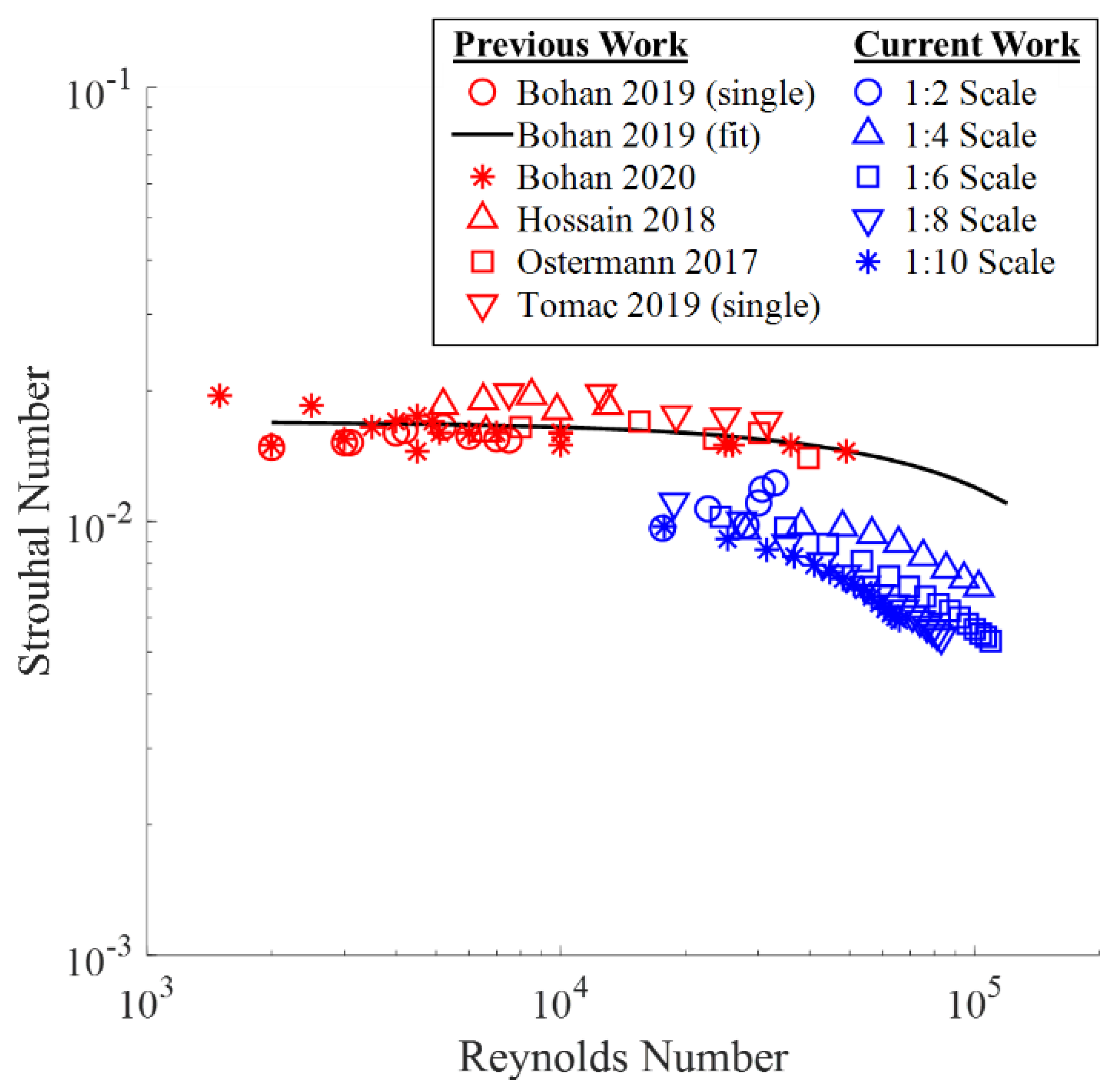
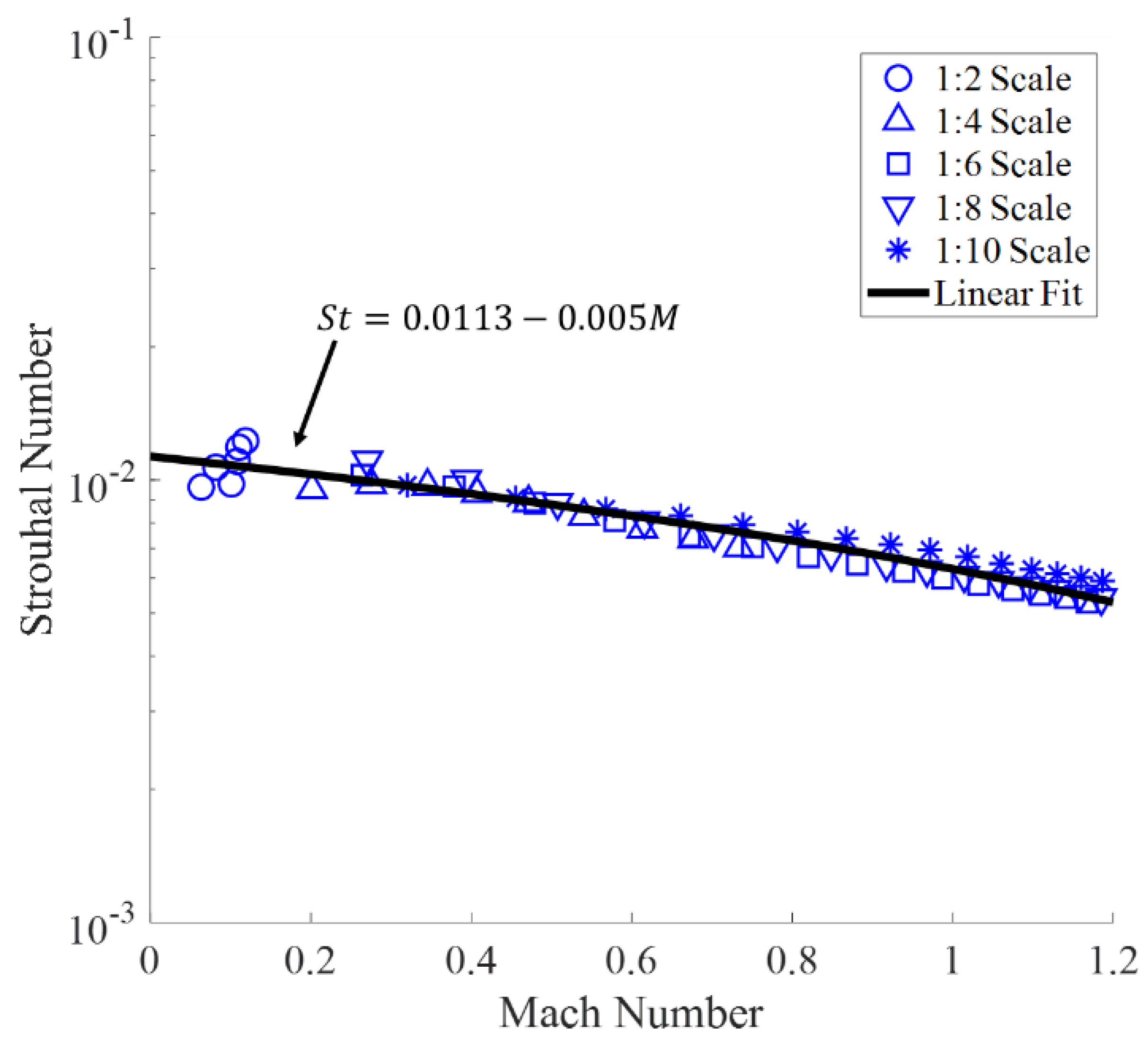
3.1. Oscillation Frequencies

A non-dimensional comparison between the oscillation frequencies and flow rates for all fluidic oscillator scales can be seen in Figure 5, which also includes results from previous research [18,30,31,32,33]. While the Strouhal numbers that were calculated in this study were lower than the previously reported data, they were on the same order of magnitude and followed the same trend relative to the Reynolds number [30]. The slight disparity (ΔSt < 0.01) between prior data and the data in this study could stem from the fact that all previously reported work calculated the bulk velocity of the sweeping jet based on a known inlet mass flow rate and the assumption of incompressible flow.

Another non-dimensional comparison between oscillation frequencies and flow rates can be seen in Figure 6, where the Strouhal numbers were compared to the Mach numbers of each trial. The linear fit (R² = 0.93) in Figure 6 shows that the Strouhal numbers were directly correlated to the Mach number, regardless of the scale of the fluidic oscillator. This linear fit also closely matched the fit that was proposed by Oz and Kara, whose computational results in the compressible flow regime showed that St ≈ 0.013 when M < 1 [14]. The linear relationship between the Strouhal number and Mach number that is observed in this study demonstrates that the oscillating behavior depends primarily on the mass flow rate of the air.

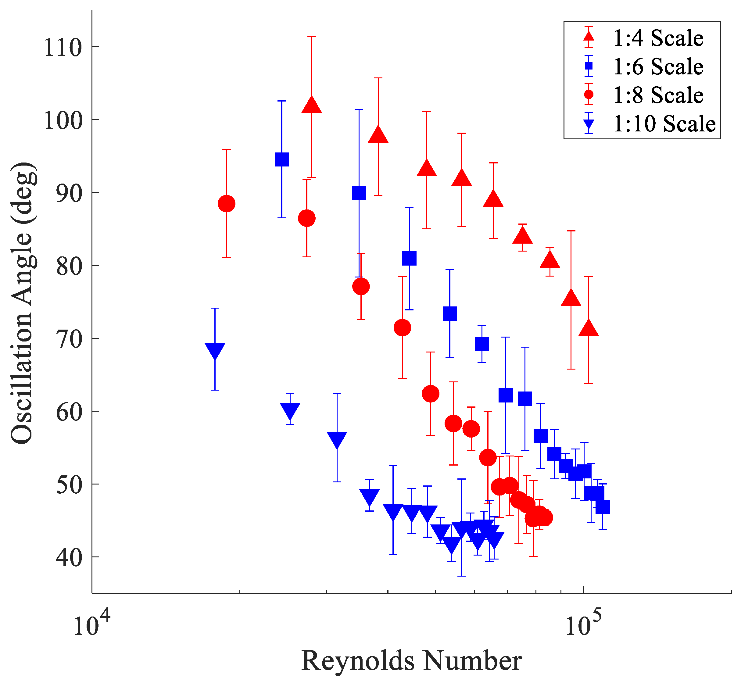
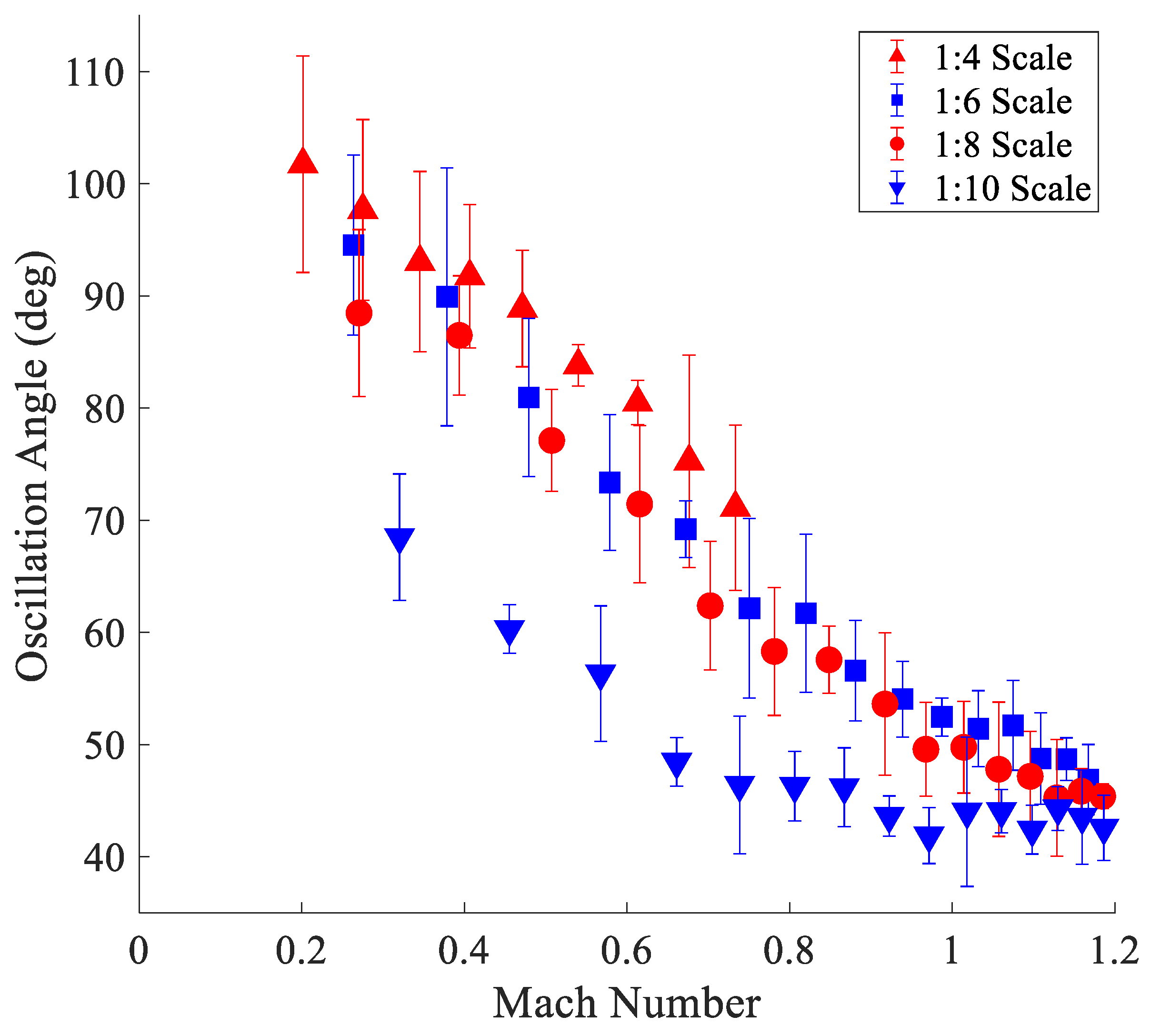
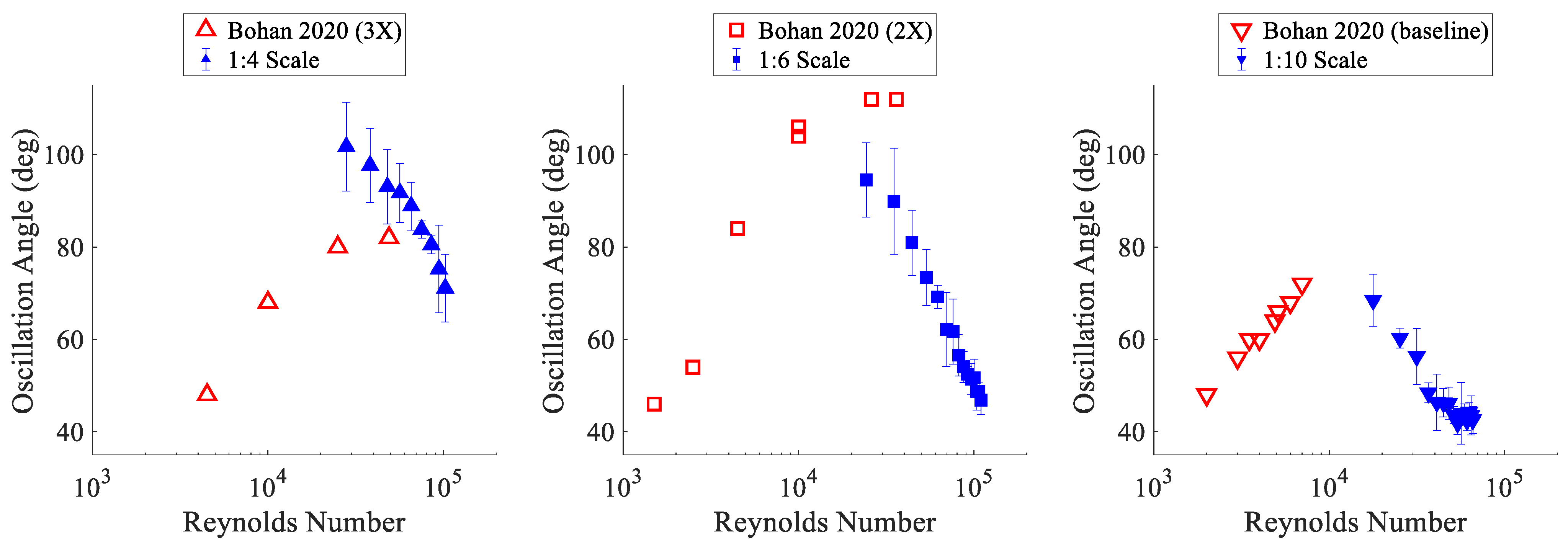
3.2. Oscillation Angles

A comparison between the oscillation angles and Reynolds numbers for each fluidic oscillator scale can be seen in Figure 7, where the error bars for the oscillation angle values represent two standard deviations from the mean of the trial’s data (n = 5). It should be noted that the low contrast within the Schlieren images that were captured for the 1:2 scale fluidic oscillator led to unreliable measurements of the oscillation angles, so any data depending on the 1:2 scale oscillation angles were excluded. Figure 7 shows that the oscillation angle had an inverse correlation to the Reynolds number for all the fluidic oscillator scales. The same inverse correlation was observed when the oscillation angles were compared to the Mach numbers, as shown in Figure 8. However, the results in Figure 8 also show that the scale of a fluidic oscillator had little influence on the oscillation angle’s relationship to the Mach number. The disparity between the results from the 1:10 scale and the other scales supports the findings from Koklu, which showed a decrease in the fluidic oscillator performance at that scale [34]. This disparity, which has been explained by Melton et al., is caused by the jet not attaching to the walls of the mixing chamber [4]. It should also be noted that Bobusch et al. reported that the diverging nozzle (after the exit throat) did not affect the oscillation frequency or angle [35].

The inverse relationship between the oscillation angle and flow rate that is observed in this study does not support the findings of Bohan et al., which reported an increase in oscillation angle as the flow rate increased [18]. The fluidic oscillator scales that had the closest exit throat diameters to the fluidic oscillators used by Bohan et al. are compared in Figure 9. It should be noted that the Bohan et al. data presented in that figure utilized carbon dioxide as the working fluid [18]. The apparent increase, and subsequent decrease, in oscillation angles as the flow rate increases is further discussed in the following sections. However, this finding ultimately demonstrates the possibility of a fluidic oscillator having a maximum sweep angle.

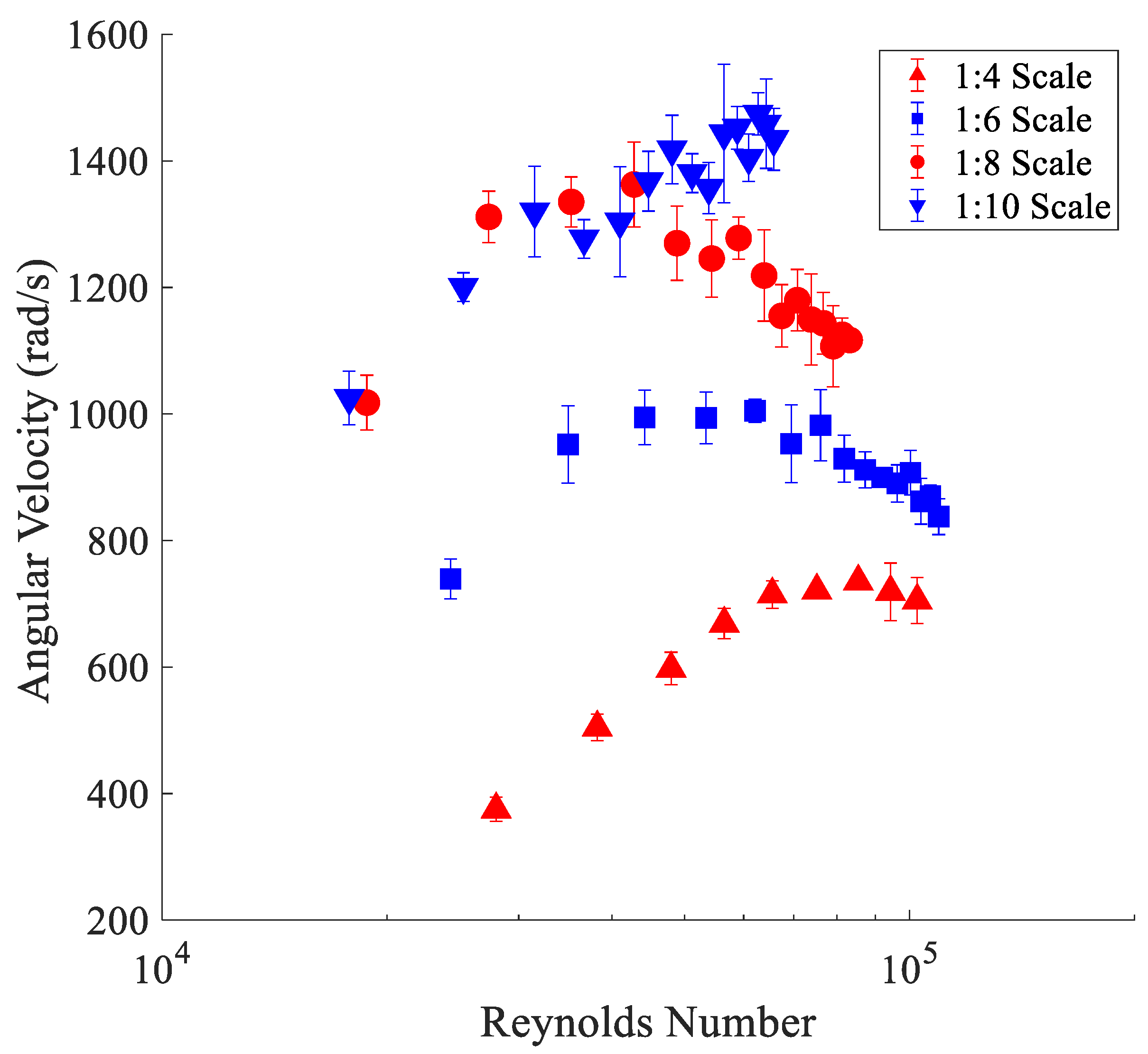
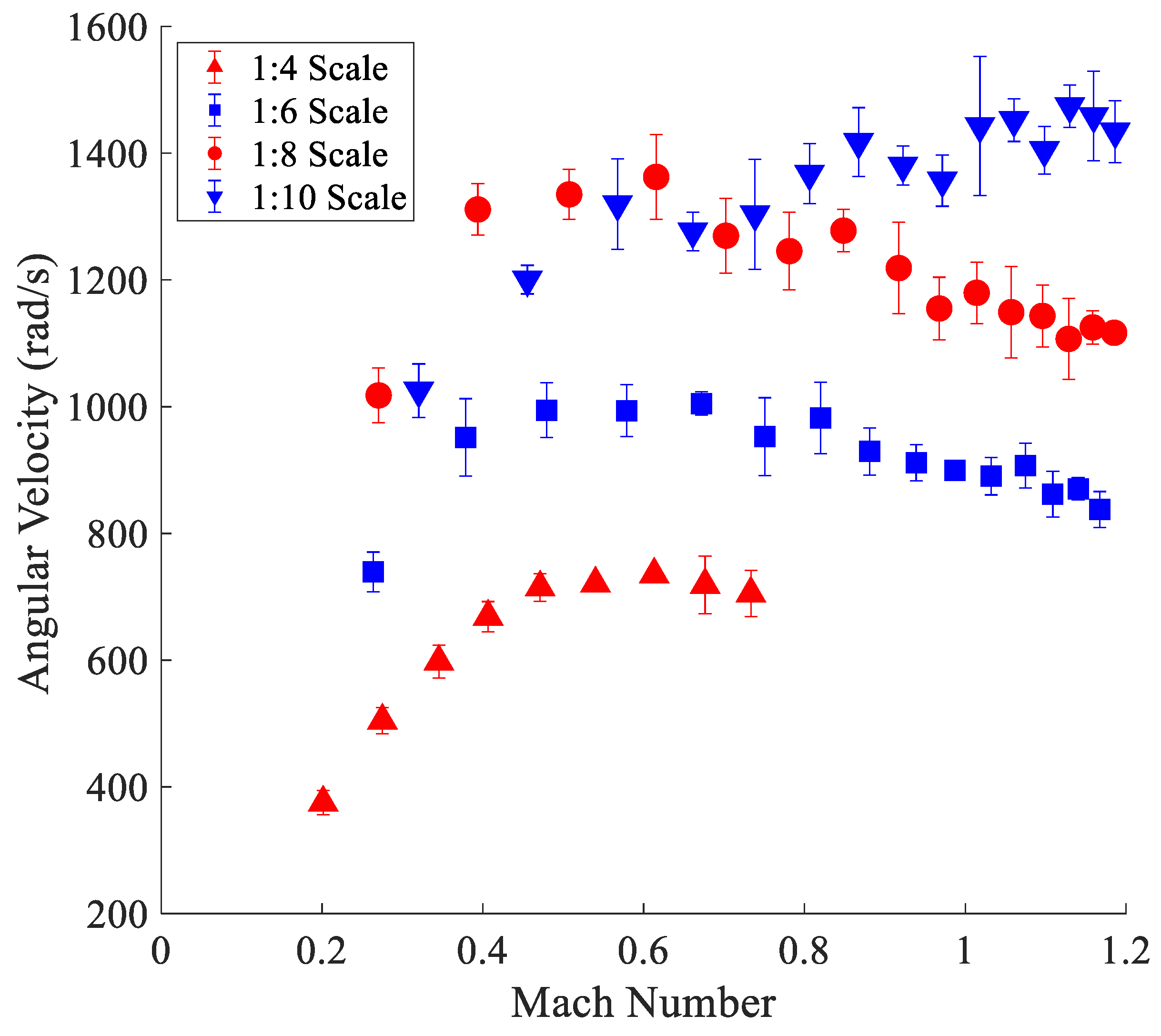
3.3. Angular Velocities

The angular velocities of the sweeping jets from the various fluidic oscillator scales are shown in Figure 10 and Figure 11, where they are compared to the Reynolds and Mach numbers, respectively. The error bars in these figures stem from the uncertainties in the oscillation frequencies and oscillation angles. Figure 10 and Figure 11 show that there is a nonlinear relationship between the angular velocity and the flow rate, and what appears to be a relative maximum angular velocity. However, similar to previous results, there was some disparity in the trends that were observed with the 1:10 scale. Moreover, while the maximum angular velocity for each scale occurred at different Reynolds numbers, they appeared to occur around the same Mach number, 0.6.

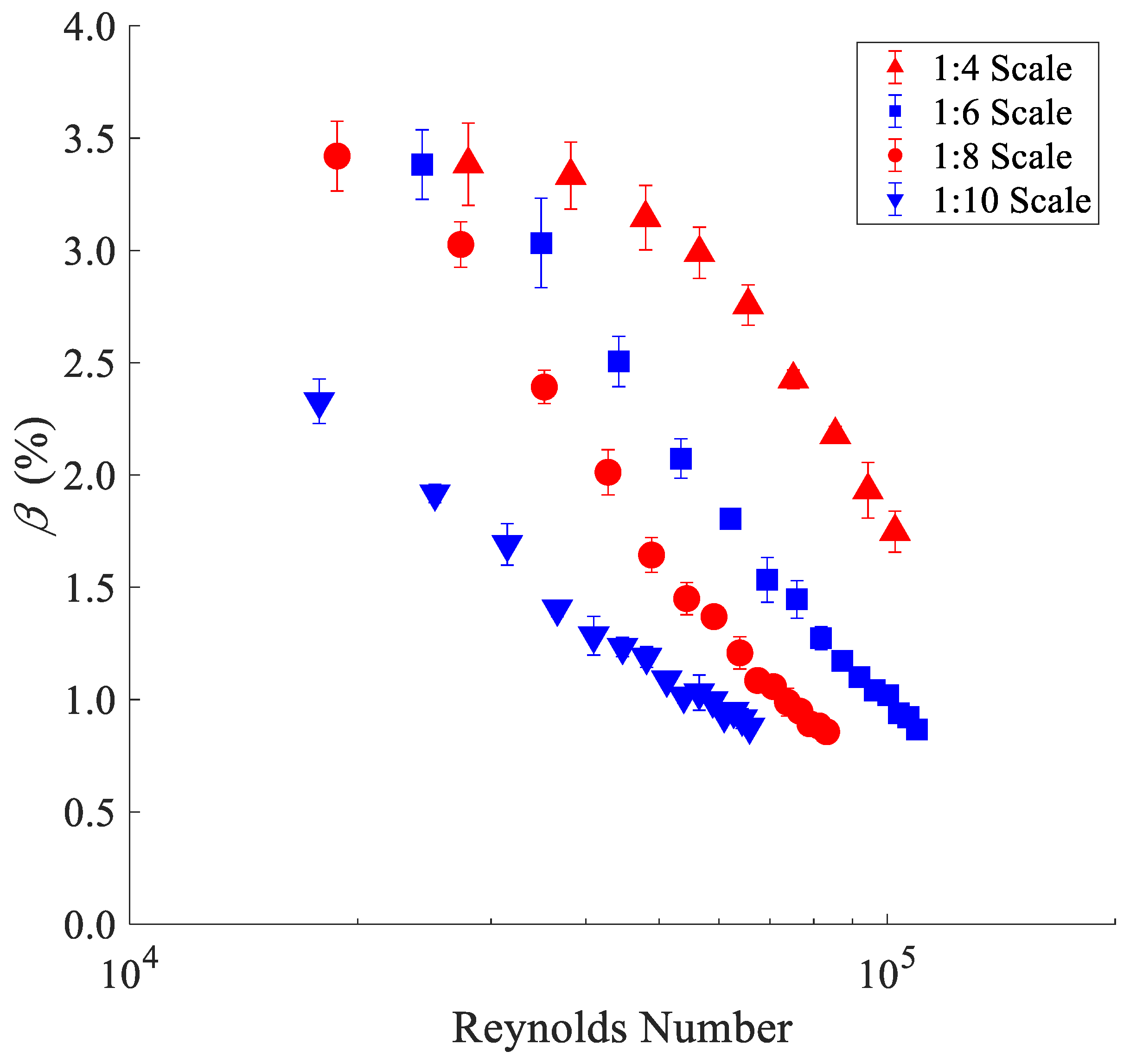
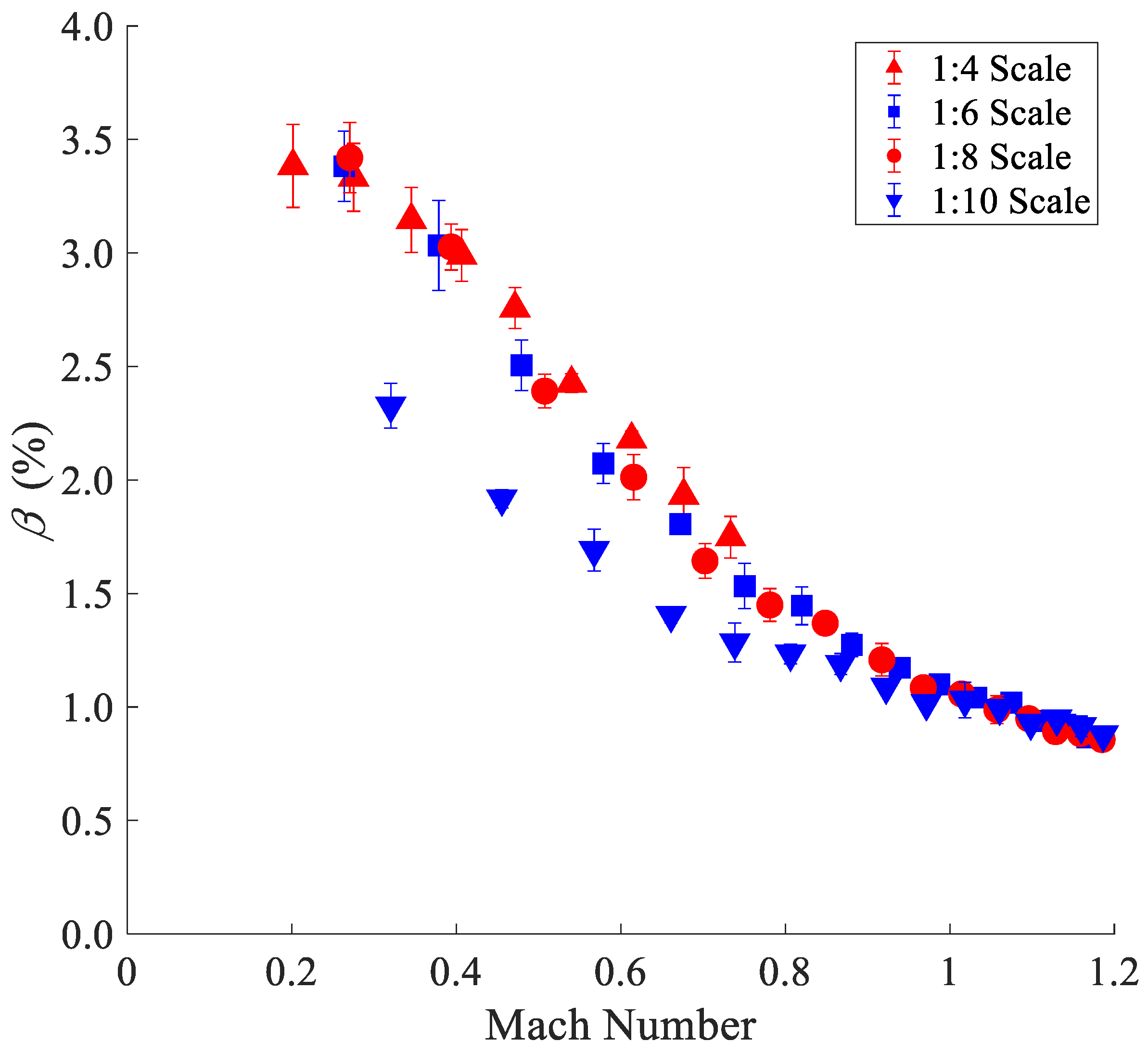
3.4. Velocity Ratios

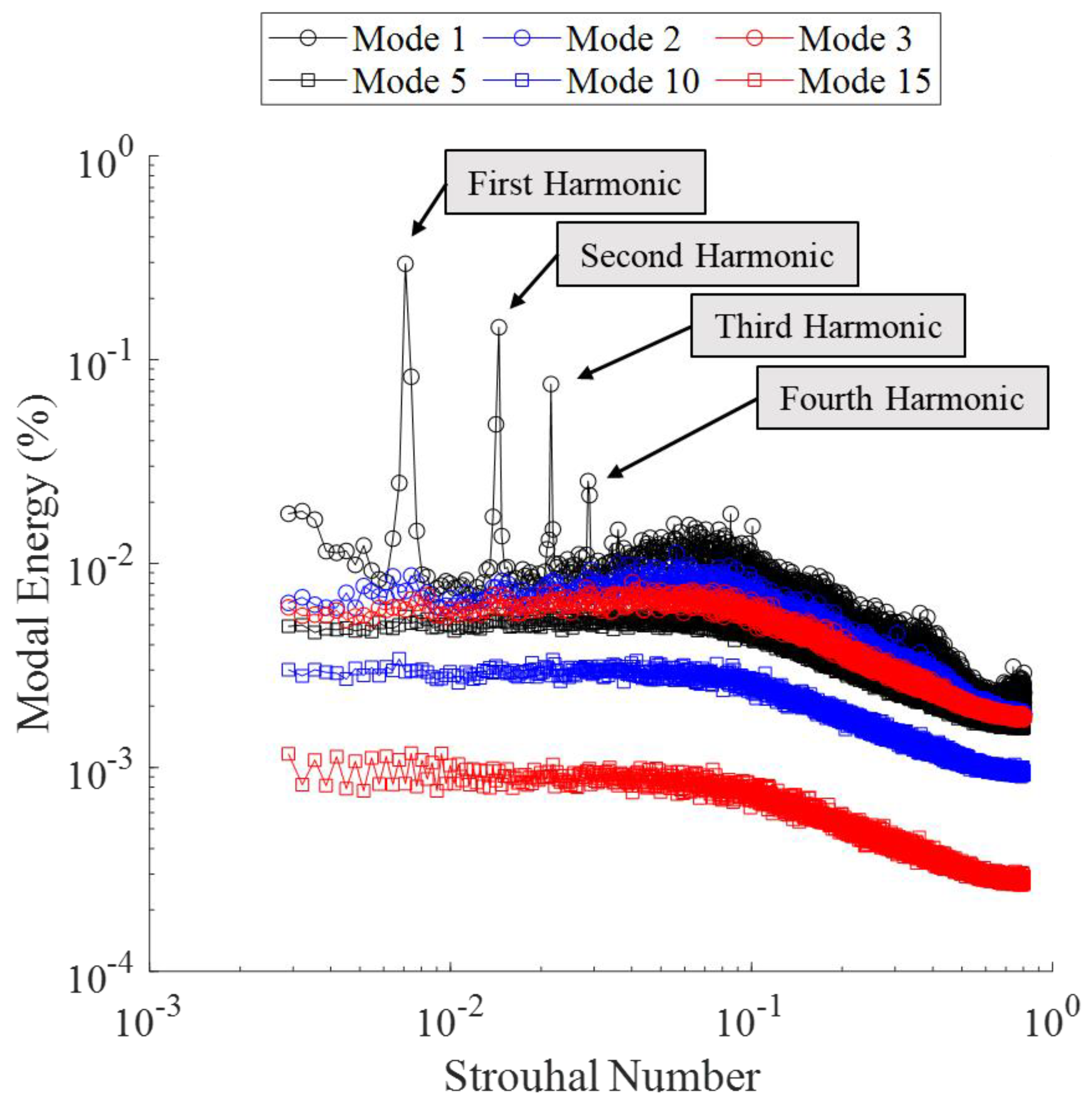
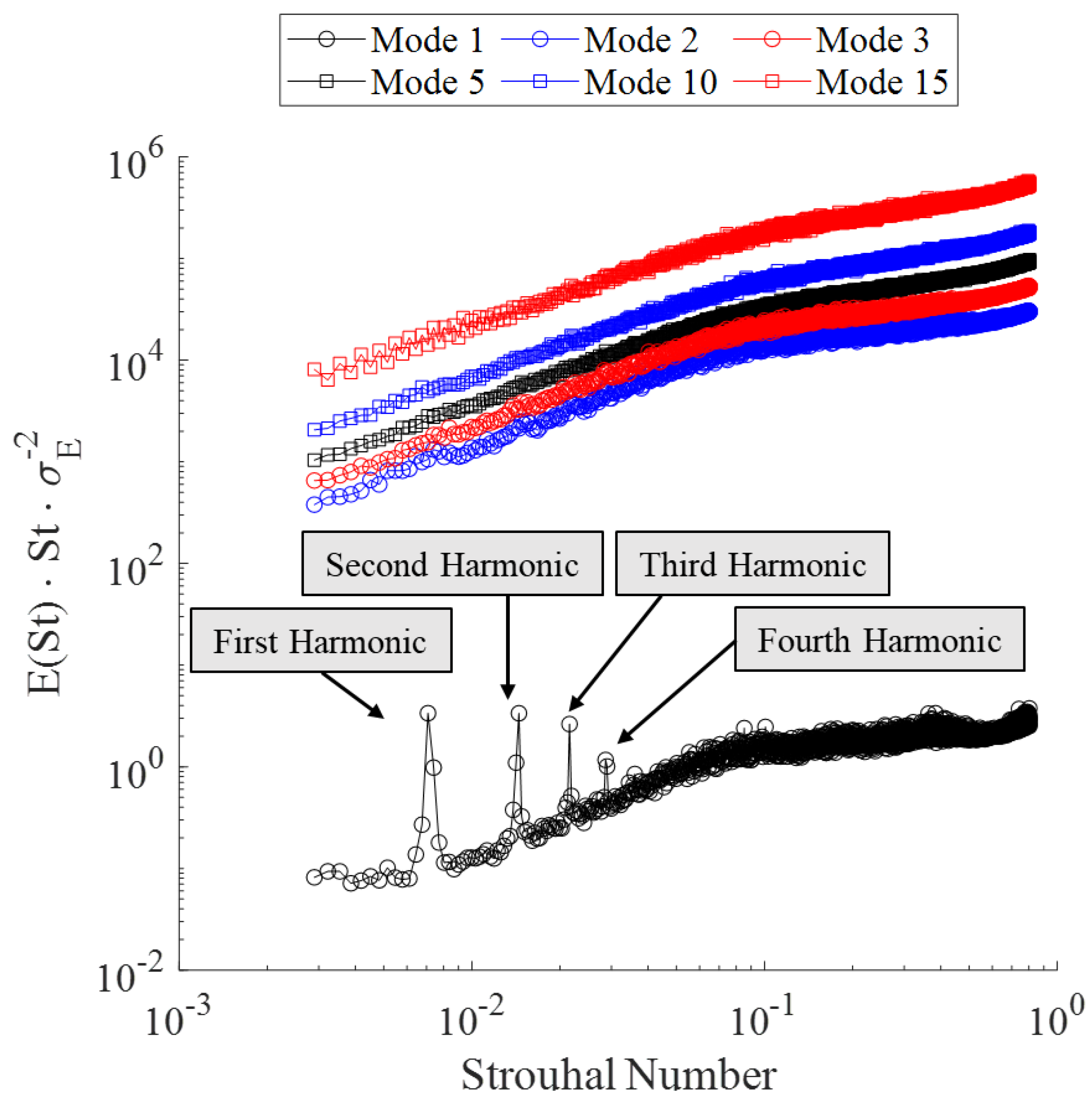
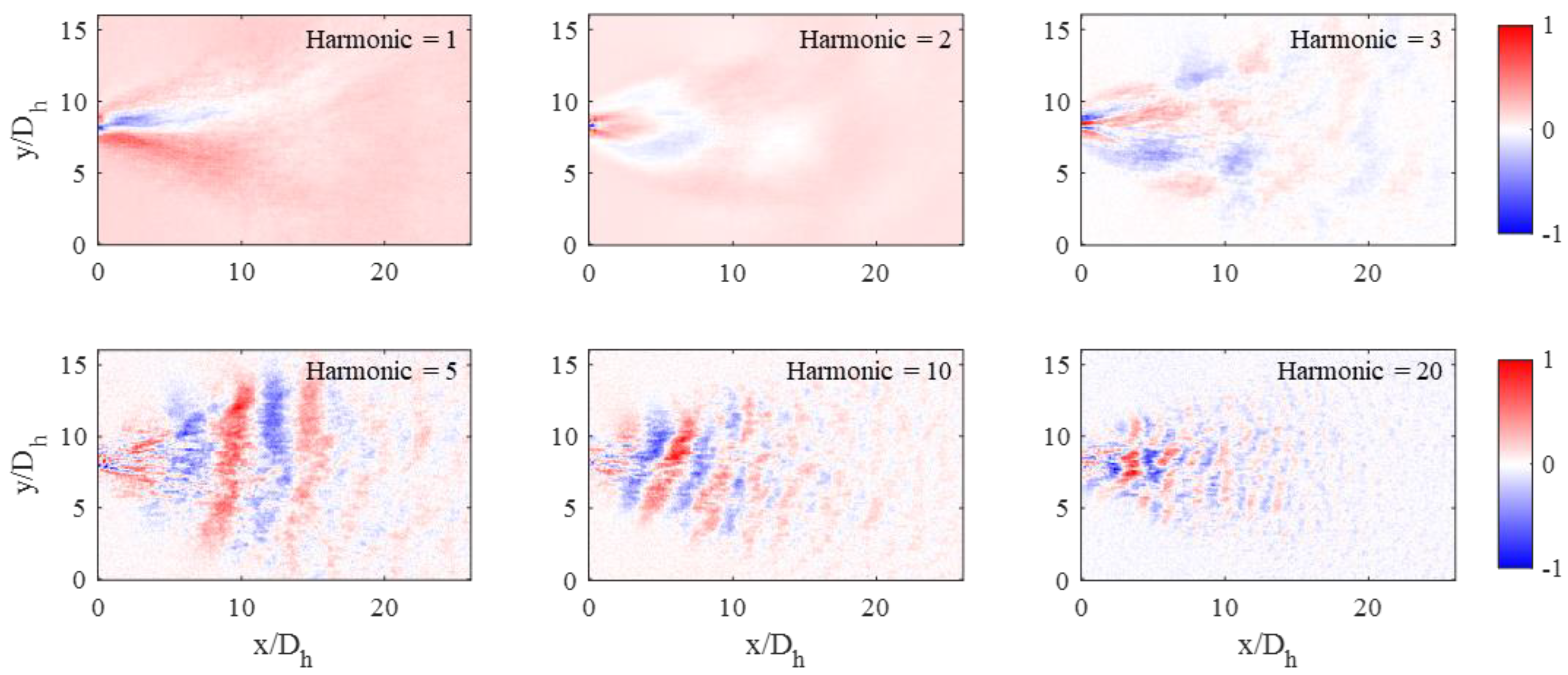
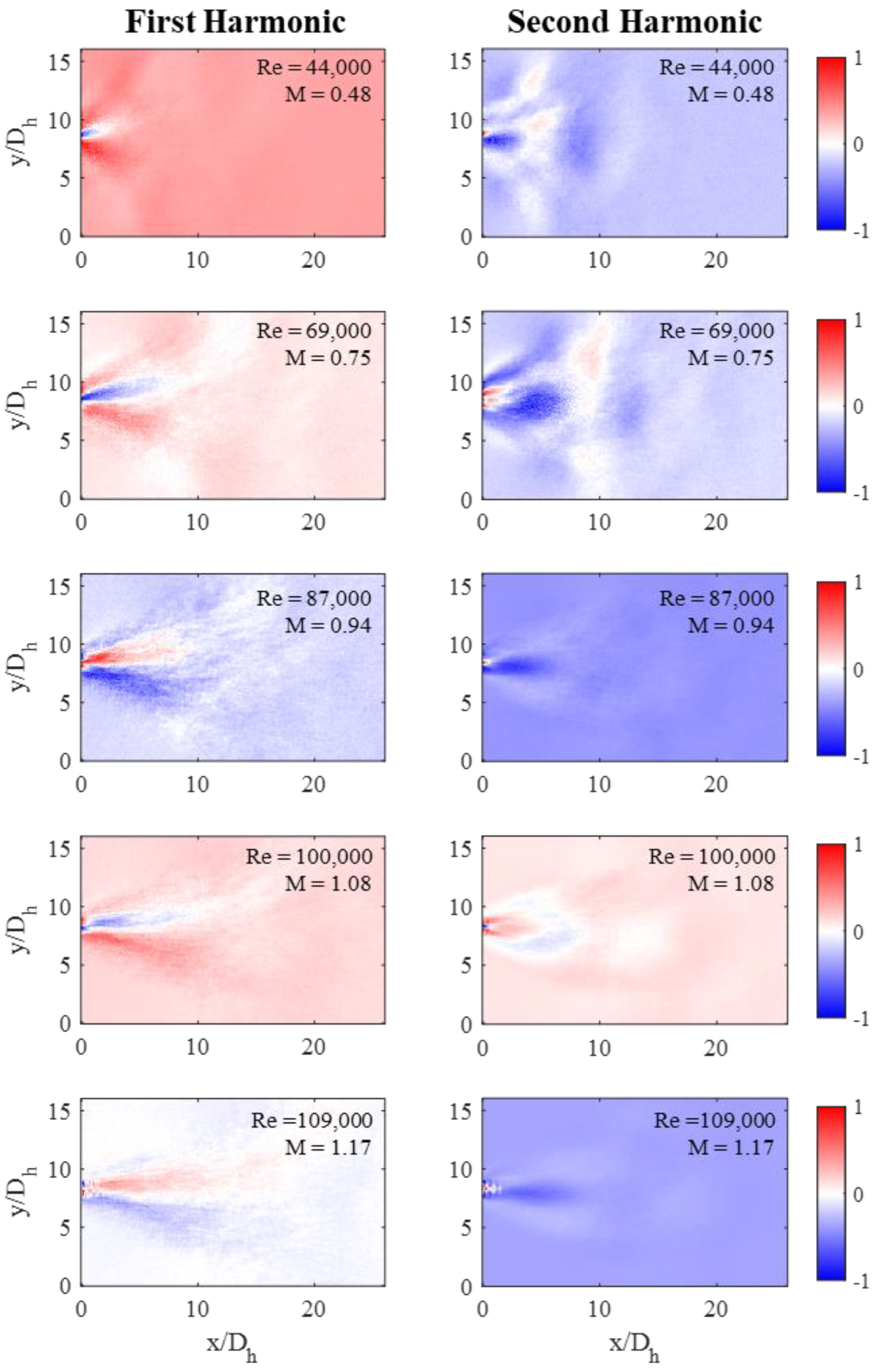
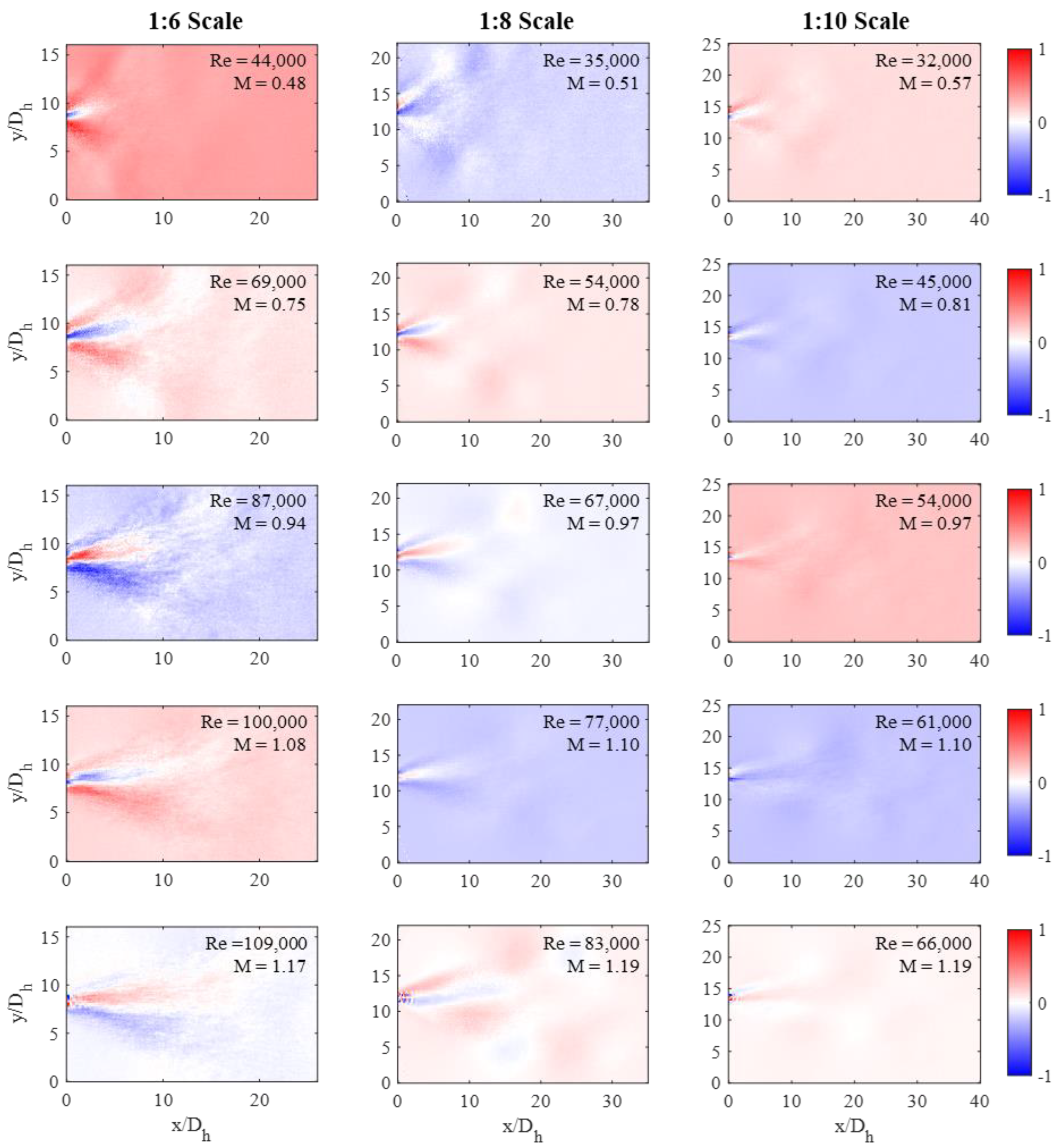
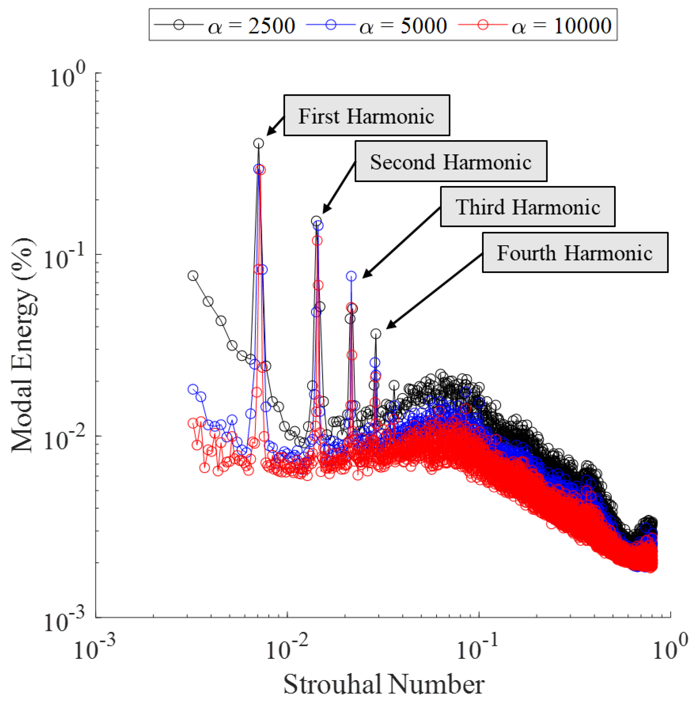
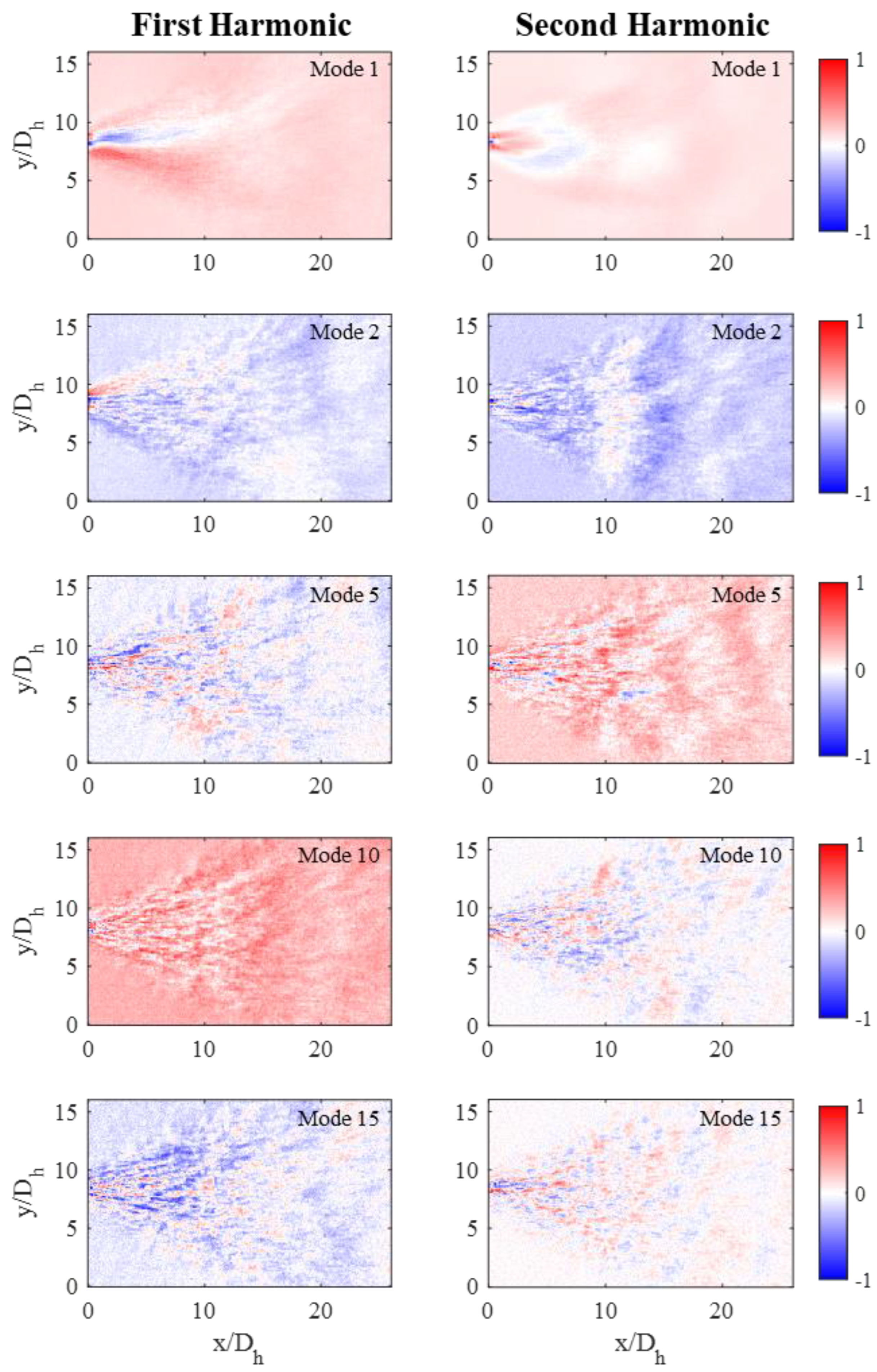
The conceptual model that is described in this section was developed to explain the observed increase, then decrease, of oscillation angles and angular velocities with respect to increasing flow rates. At an extremely low Reynolds number, the laminar flow moving through the fluidic oscillator would produce a small, if not negligible, sweeping pattern. Then, if the flow rate progressively increased, the momentum of the jet (perpendicular to the inlet flow) would also increase and sweep further from side to side. However, at even higher flow rates, the momentum of the jet (in the direction parallel to the inlet flow) would begin to dominate the oscillatory motion, thus preventing the jet from sweeping as widely.

To validate this conceptual model, the ratio of the angular velocity to the total velocity of the jet was evaluated for increasing flow rates. These results can be seen in Figure 12 and Figure 13, which demonstrate that the angular velocity becomes less influential towards the jet’s sweeping motion. The error bars in these figures stem from the uncertainties in the oscillation frequencies, oscillation angles, and air velocities. The data in Figure 13 also support the decrease in performance at the 1:10 scale that is observed in Figure 8 and by Koklu [34].

3.5. Modal Analysis

For the modal analysis, five inlet pressures were supplied to the 1:6, 1:8, and 1:10 scale fluidic oscillators: 143, 184, 225, 267, and 308 kPa (6, 12, 18, 24, and 30 psig). The Schlieren image sets for each trial consisted of 50,000 images (320 × 200 pixels) that were recorded at 100 kHz. To ensure the validity of the SPOD results, a sensitivity analysis was conducted to determine the appropriate number of images per image block (α). Three image block sizes (2500, 5000, and 10,000) with an overlap of 50% were evaluated. The power spectral density (PSD) of Mode 1 for each of the image block sizes can be seen in Figure 14; these results were attained using images from the 1:6 scale at an inlet pressure of 184 kPa (12 psig).

Figure 14 shows that the SPOD results were not significantly influenced by the image block sizes. However, since smaller image blocks result in lower frequency resolution and larger image blocks result in lower quantities of modes, the 5000-image block size was used for all SPOD analyses. These block sizes provided a frequency resolution of 20 Hz across 19 modes.

All the mode structures that were analyzed in this study were selected based on the PSD data that were calculated for each trial. An example of PSD data can be seen in Figure 15 and Figure 16, which show the PSD of the 1:6 scale at an inlet pressure of 184 kPa. Figure 15 compares the modal energy, as a percentage of the total energy, to the dimensionless frequency for different modes. A similar PSD comparison can be seen in Figure 16, where the modal energy was normalized with the Strouhal numbers and standard deviation of the energy in each mode (σ_E). The Mode 1 data in Figure 14, Figure 15 and Figure 16 show peaks at specific frequencies, and after further analysis, it was observed that those peaks correspond to harmonics of the oscillation frequency.

Once the harmonic frequencies had been identified, the structures at those frequencies for different modes were evaluated. An example of mode structures at the same harmonic frequencies can be seen in Figure 17, which depicts the 1:6 scale operating with an inlet pressure of 267 kPa (24 psig). Since the modal energy decreases as the mode number increases, the mode structures become less defined, because they represent flow structures with a lower energy content. It should be noted that all the mode structures that are shown in this work depict the real values of the complex results and are spatially normalized to the exit throat diameter of the respective fluidic oscillator scale. The magnitudes of all the mode structures are also scaled between −1 and 1 to improve visual comparisons.

Different harmonic frequencies within the same mode were also evaluated, and an example from Mode 1 of the 1:6 scale operating with an inlet pressure of 267 kPa (24 psig) can be seen in Figure 18. While the mode structures at lower frequencies depict the sweeping motion of the jet, the mode structures at higher frequencies depict smaller-scale turbulence structures, which is to be expected, as the energy content of those modes is lower. However, it should be noted that the structures occurring at the harmonic frequencies have a larger scale than those occurring at neighboring frequencies. The trends that were observed across modes and harmonic frequencies were observed for all fluidic oscillator scales and flow rates.

The harmonic mode structures of each fluidic oscillator scale were then compared across flow rates. Figure 19 shows structures from the first two harmonics (of Mode 1) of the 1:6 scale at the five flow rates. The first harmonic mode structures show the jet at its maximum sweep positions and show opposing and symmetric correlations on either side of the centerline of the fluidic oscillator. While the second harmonic mode structures also showed physical symmetry across the same axis, they had symmetric correlations as well. Both sets of mode structures showed that the jet’s oscillation angle decreased and its distance from the fluidic oscillator increased as the flow rate increased.

The first harmonic mode structures (of Mode 1) were then compared across fluidic oscillator scales and flow rates, as shown in Figure 20. The same symmetric and inversely correlated structures that are observed in Figure 19 can be seen across the fluidic oscillator scales and flow rates. The mode structures in Figure 20 extend less than 10 exit diameters from the fluidic oscillator at the lowest flow rates and reach almost 20 exit diameters at the highest flow rates. The spatial growth of the mode structures in the x-direction is caused by an increase in the mass and velocity or momentum of the jet at the higher flow rates. Moreover, as noted by the Reynolds numbers, the mode structures appear to have less turbulence as the scale decreases.

4. Discussion

The objective of this study was to evaluate the performance of a single fluidic oscillator design across different scale sizes and air flow rates that were in the compressible flow regime. While previous groups, which assumed incompressible flow, reported oscillation frequencies that produced Strouhal numbers between 0.010–0.020, this study showed that the Strouhal number decreased from approximately 0.013 to 0.005 as the flow rates approached supersonic flow. The Strouhal number was directly correlated to the Mach number (St = 0.0113–0.005M) and did not depend on the scale size of the fluidic oscillator.

Contrary to the findings of Bohan et al., which reported an increase in oscillation angles with respect to increasing flow rates, the results of this study showed that the oscillation angle decreased as the flow rate increased [18]. The oscillation angles, regardless of scale, were directly correlated to the Mach number, and displayed a decrease and plateau as they approached and entered the supersonic flow regime. However, the 1:10 scale fluidic oscillator exhibited smaller sweep angles (relative to the other scales), which supports the performance reduction that was reported by Koklu at that scale [34]. In this study, the decrease in oscillation angles at higher flow rates was attributed to a decrease in the jet’s angular momentum, relative to its linear momentum, as it exited the fluidic oscillator. The ratio of the angular velocity of the jet to the total velocity of the jet was directly correlated to the Mach number, regardless of the scale (also with the exception of the 1:10 scale). The angular velocities of the 1:4, 1:6, and 1:8 scales all exhibited maximums at approximately M = 0.6.

While the SPOD results further validated the oscillation frequencies and oscillation angles, they also identified the mode structures (and their energy content) that occurred at the harmonics of the oscillation frequencies. The mode structures were evaluated at identical frequencies, and as the mode number increased, the resolution of the mode structures decreased. When mode structures were evaluated for different harmonic frequencies with the same mode number, the mode structures depicted smaller-scale turbulence within the flow field. The mode structures with the highest energy content from the 1:6, 1:8, and 1:10 fluidic oscillator scales were compared to each other, and displayed similar mode structures resembling the jet at its fullest sweep position. As the flow rate increased for each scale, the mode structures extended further beyond the fluidic oscillator.

The findings in this study demonstrate that the oscillation frequency, oscillation angle, angular velocity of the jet, and high-energy mode structures that are produced by a fluidic oscillator can be accurately predicted if the fluidic oscillator scale and gas flow rate are known. The ability to predict fluidic oscillator performance can significantly improve the design process for an application where a fluidic oscillator may be used.

References

1. Tritton, D.J. Physical Fluid Dynamics; Springer Science & Business Media: Berlin/Heidelberg, Germany, 2012. [Google Scholar]
2. Bauer, P. Oscillator and Shower Head for Use Therewith. U.S. Patent 3563462, 16 February 1971. [Google Scholar]
3. Hossain, M.A.; Ameri, A.; Gregory, J.W.; Bons, J. Effects of Fluidic Oscillator Nozzle Angle on the Flowfield and Impingement Heat Transfer. AIAA J. 2021, 59, 2113–2125. [Google Scholar] [CrossRef]
4. Melton, L.P.; Koklu, M.; Andino, M.; Lin, J.C.; Edelman, L.M. Sweeping jet optimization studies. In Proceedings of the 8th AIAA Flow Control Conference, Washington, DC, USA, 13–17 June 2016; p. 4233. [Google Scholar]
5. Hossain, M.A.; Asar, M.E.; Gregory, J.W.; Bons, J.P. Experimental Investigation of Sweeping Jet Film Cooling in a Transonic Turbine Cascade. J. Turbomach. 2020, 142, 041009. [Google Scholar] [CrossRef]
6. Liebsch, J.; Paschereit, C.O. Oscillating Wall Jets for Active Flow Control in a Laboratory Fume Hood—Experimental Investigations. Fluids 2021, 6, 279. [Google Scholar] [CrossRef]
7. Xia, L.; Hua, Y.; Zheng, J. Numerical investigation of flow separation control over an airfoil using fluidic oscillator. Phys. Fluids 2021, 33, 065107. [Google Scholar] [CrossRef]
8. Koklu, M. Performance Assessment of Fluidic Oscillators Tested on the NASA Hump Model. Fluids 2021, 6, 74. [Google Scholar] [CrossRef]
9. Seele, R.; Tewes, P.; Woszidlo, R.; McVeigh, M.A.; Lucas, N.J.; Wygnanski, I.J. Discrete sweeping jets as tools for improving the performance of the V-22. J. Aircr. 2009, 46, 2098–2106. [Google Scholar] [CrossRef]
10. Tewes, P.; Taubert, L.; Wygnanski, I. On the use of sweeping jets to augment the lift of a lambda-wing. In Proceedings of the 28th AIAA Applied Aerodynamics Conference, Chicago, IL, USA, 28 June–1 July 2010; p. 4689. [Google Scholar]
11. Kim, S.-H.; Kim, K.-Y. Effects of installation location of fluidic oscillators on aerodynamic performance of an airfoil. Aerosp. Sci. Technol. 2020, 99, 105735. [Google Scholar] [CrossRef]
12. Portillo, D.J.; Hoffman, E.N.; Garcia, M.; LaLonde, E.; Hernandez, E.; Combs, C.S.; Hood, L. Modal Analysis of a Sweeping Jet Emitted by a Fluidic Oscillator. In Proceedings of the AIAA Aviation 2021 Forum, Virtual Event, 2–6 August 2021; p. 2835. [Google Scholar]
13. Gosen, F.V.; Ostermann, F.; Woszidlo, R.; Nayeri, C.N.; Paschereit, C.O. Experimental investigation of compressibility effects in a fluidic oscillator. In Proceedings of the 53rd AIAA Aerospace Sciences Meeting, Kissimmee, FL, USA, 5–9 January 2015; p. 11. [Google Scholar]
14. Oz, F.; Kara, K. Jet Oscillation Frequency Characterization of a Sweeping Jet Actuator. Fluids 2020, 5, 72. [Google Scholar] [CrossRef]
15. Park, S.; Ko, H.; Kang, M.; Lee, Y. Characteristics of a Supersonic Fluidic Oscillator Using Design of Experiment. AIAA J. 2020, 58, 2784–2789. [Google Scholar] [CrossRef]
16. Bray, H.C., Jr. Cold Weather Fluidic Fan Spray Devices and Method. U.S. Patent 4,463,904, 7 August 1984. [Google Scholar]
17. Settles, G.S. Schlieren and Shadowgraph Techniques: Visualizing Phenomena in Transparent Media; Springer Science & Business Media: Berlin/Heidelberg, Germany, 2001. [Google Scholar]
18. Bohan, B.T.; Polanka, M.D. The Effect of Scale and Working Fluid on Sweeping Jet Frequency and Oscillation Angle. J. Fluids Eng. 2020, 142, 061206. [Google Scholar] [CrossRef]
19. Hirsch, D.; Gharib, M. Schlieren visualization and analysis of sweeping jet actuator dynamics. AIAA J. 2018, 56, 2947–2960. [Google Scholar] [CrossRef]
20. Taira, K.; Brunton, S.L.; Dawson, S.T.; Rowley, C.W.; Colonius, T.; McKeon, B.J.; Schmidt, O.T.; Gordeyev, S.; Theofilis, V.; Ukeiley, L.S. Modal analysis of fluid flows: An overview. AIAA J. 2017, 55, 4013–4041. [Google Scholar] [CrossRef] [Green Version]
21. Towne, A.; Schmidt, O.T.; Colonius, T. Spectral proper orthogonal decomposition and its relationship to dynamic mode decomposition and resolvent analysis. J. Fluid Mech. 2017, 847, 821–867. [Google Scholar] [CrossRef] [Green Version]
22. Schmidt, O.T.; Colonius, T. Guide to spectral proper orthogonal decomposition. AIAA J. 2020, 58, 1023–1033. [Google Scholar] [CrossRef]
23. Lumley, J.L. The structure of inhomogeneous turbulent flows. Atmos. Turbul. Radio Wave Propag. 1967, 166–178. [Google Scholar]
24. Schmid, P.J. Dynamic mode decomposition of numerical and experimental data. J. Fluid Mech. 2010, 656, 5–28. [Google Scholar] [CrossRef] [Green Version]
25. Glauser, M.N.; Leib, S.J.; George, W.K. Coherent structures in the axisymmetric turbulent jet mixing layer. In Turbulent Shear Flows 5; Springer: Berlin/Heidelberg, Germany, 1987; pp. 134–145. [Google Scholar]
26. Sinha, A.; Rodríguez, D.; Brès, G.A.; Colonius, T. Wavepacket models for supersonic jet noise. J. Fluid Mech. 2014, 742, 71–95. [Google Scholar] [CrossRef] [Green Version]
27. Schmidt, O.T.; Towne, A.; Rigas, G.; Colonius, T.; Brès, G.A. Spectral analysis of jet turbulence. J. Fluid Mech. 2018, 855, 953–982. [Google Scholar] [CrossRef] [Green Version]
28. Cottier, S.; Combs, C.S.; Vanstone, L. Spectral Proper Orthogonal Decomposition Analysis of Shock-Wave/Boundary-Layer Interactions. In Proceedings of the AIAA Aviation 2019 Forum, Dallas, TX, USA, 17–21 June 2019; p. 3331. [Google Scholar]
29. Hoffman, E.N.; Rodriguez, J.M.; Cottier, S.M.; Combs, C.S.; Bathel, B.F.; Weisberger, J.M.; Jones, S.B.; Schmisseur, J.D.; Kreth, P.A. Modal Analysis of Cylinder-Induced Transitional Shock-Wave/Boundary-Layer Interaction Unsteadiness. AIAA J. 2022, 60, 2730–2748. [Google Scholar] [CrossRef]
30. Bohan, B.T.; Polanka, M.D.; Rutledge, J.L. Sweeping jets issuing from the face of a backward-facing step. J. Fluids Eng. 2019, 141, 121201. [Google Scholar] [CrossRef]
31. Hossain, M.A.; Ameri, A.; Gregory, J.W.; Bons, J.P. Sweeping jet impingement heat transfer on a simulated turbine vane leading edge. J. Glob. Power Propuls. Soc. 2018, 2, 402–414. [Google Scholar] [CrossRef]
32. Ostermann, F.; Woszidlo, R.; Nayeri, C.; Paschereit, C.O. Effect of velocity ratio on the flow field of a spatially oscillating jet in crossflow. In Proceedings of the 55th AIAA Aerospace Sciences Meeting, Grapevine, TX, USA, 9–13 January 2017; p. 0769. [Google Scholar]
33. Tomac, M.N.; Gregory, J.W. Phase-synchronized fluidic oscillator pair. AIAA J. 2019, 57, 670–681. [Google Scholar] [CrossRef]
34. Koklu, M. Effects of sweeping jet actuator parameters on flow separation control. AIAA J. 2018, 56, 100–110. [Google Scholar] [CrossRef] [PubMed]
35. Bobusch, B.B.; Woszidlo, R.; Kruger, O.; Paschereit, C.O. Numerical investigations on geometric parameters affecting the oscillation properties of a fluidic oscillator. In Proceedings of the 21st AIAA Computation Fluid Dynamics Conference, San Diego, CA, USA, 24–27 June 2013. [Google Scholar]
Figure 1. A fluidic oscillator at various phase angles (Φ); dominant flow direction is left to right.
Fluids 07 00251 g001
Figure 2. Dimensioned (mm) fluidic oscillator baseline geometry, which was raised to a height of the exit throat diameter (25 mm); also depicts the location of the pitot static probe.
Fluids 07 00251 g002
Figure 3. CAD rendering of the Schlieren imaging setup.
Fluids 07 00251 g003
Figure 4. Example of the maximum, minimum, and absolute difference of pixel intensities across an image set; depicts data from the 1:8 scale at an inlet pressure of 198 kPa (14 psig).
Fluids 07 00251 g004
Figure 5. Strouhal number versus Reynolds number across fluidic oscillator scales, including prior data [18,30,31,32,33].
Fluids 07 00251 g005
Figure 6. Strouhal number versus Mach number across fluidic oscillator scales.
Fluids 07 00251 g006
Figure 7. Oscillation angle versus Reynolds number across fluidic oscillator scales.
Fluids 07 00251 g007
Figure 8. Oscillation angle versus Mach number across fluidic oscillator scales.
Fluids 07 00251 g008
Figure 9. Oscillation angle versus Reynolds number compared to equivalently sized fluidic oscillators in prior publication by Bohan et al. [18].
Fluids 07 00251 g009
Figure 10. Angular velocity versus Reynolds number across fluidic oscillator scales.
Fluids 07 00251 g010
Figure 11. Angular velocity versus Mach number across fluidic oscillator scales.
Fluids 07 00251 g011
Figure 12. Ratio between angular velocity and total velocity (β) versus Reynolds number across fluidic oscillator scales.
Fluids 07 00251 g012
Figure 13. Ratio between angular velocity and total velocity (β) versus Mach number across fluidic oscillator scales.
Fluids 07 00251 g013
Figure 14. Modal energy as a percentage of total energy versus Strouhal numbers for various image block sizes (α); showing data from the 1:6 scale at an inlet pressure of 184 kPa (12 psig).
Fluids 07 00251 g014
Figure 15. Modal energy as a percentage of total energy versus Strouhal numbers; showing data from the 1:6 scale at an inlet pressure of 184 kPa (12 psig).
Fluids 07 00251 g015
Figure 16. Normalized modal energy versus Strouhal numbers; showing data from the 1:6 scale at an inlet pressure of 184 kPa (12 psig).
Fluids 07 00251 g016
Figure 17. Different mode structures at the same harmonic frequencies; showing data from the 1:6 scale operating with an inlet pressure of 267 kPa (24 psig).
Fluids 07 00251 g017
Figure 18. Different harmonic frequencies within the same mode; showing data from Mode 1 of the 1:6 scale operating with an inlet pressure of 267 kPa (24 psig).
Fluids 07 00251 g018
Figure 19. Mode structures at the first and second harmonic frequencies (of Mode 1) of the 1:6 scale for various flow rates.
Fluids 07 00251 g019
Figure 20. Mode structures at the first harmonic frequency (of Mode 1) for the 1:6, 1:8, and 1:10 scales for various flow rates.
Fluids 07 00251 g020