Note on the Early Thermoelastic Stage Preceding Rayleigh–Bénard Convection in Soft Materials

Abstract

In this paper, we focus on the first stage of transition to Rayleigh–Bénard convection in soft-jammed systems (yield stress fluids) confined in a parallelepiped box heated from the bottom. Up to yielding, the material is in a solid-state with a constant elastic modulus. By means of a linear thermoelastic model, an analytical solution for stresses and strains induced by the gravity and the temperature gradient is derived. The analytical solution allows us to emphasize the appropriate dimensionless parameters. The onset of plastic deformation is then investigated using the classical yield criteria (Tresca, von Mises and Drucker–Prager). This analysis is subsequently applied to experimental data of the literature dealing with Rayleigh–Bénard convection in Carbopol micro gels.

1. Introduction

When a horizontal fluid layer is heated from below and cooled from above, a density stratification appears because of the thermal expansion of the fluid. The fluid at the bottom will be lighter than the fluid at the top, and this top-heavy arrangement is potentially unstable. When the temperature difference between the bottom and the top exceeds a threshold value controlled by the viscosity and heat diffusivity, by a small amount, convection sets in. The balance between buoyancy and viscous and thermal diffusion is described by the Rayleigh number:

$$\begin{array}{c}\hfill Ra=\frac{\rho g\alpha \mathsf{\Delta }T{H}^3}{\eta D_t},\end{array}$$

(1)

where $\rho$ is the fluid density, g is the acceleration due to gravity, $\mathsf{\Delta }T$ is the temperature difference between the bottom and top walls, H is the width of the fluid layer, $\alpha$ is the volume expansion coefficient, $\eta$ is the viscosity, and $D_t$ is the thermal diffusivity.

Yield stress fluids represent a large class of materials that displays a solid-like behavior as long as the applied stress does not exceed a critical value (${\tau }_y$, called a yield stress) and displays a fluid-like behavior beyond this threshold. The physical origin of the yield stress is related to the microscopic nature of these systems (soft objects suspensions, polymer solutions or emulsions). A review on yield stress fluids can be found in [1,2,3]. The onset of convection in such materials is the subject of controversy in the literature. The main theoretical and experimental results on this problem are reviewed in the following section.

1.1. Rayleigh–Bénard Convection in a Yield–Stress Fluid: Literature Review

The first theoretical study of Rayleigh–Bénard convection (RBC) in a yield stress fluid was performed by Zhang et al. [4]. They considered an inelastic yield stress fluid model (Bingham model). Using an energy method, they demonstrated that, for a finite yield stress, the basic state (conductive regime) is linearly stable at all Rayleigh numbers and is conditionally stable otherwise. In other words, convective instabilities cannot grow from a static conductive state submitted to infinitesimal perturbations regardless the finite value of the yield stress.

The same problem was studied by Balmforth and Rust [5] using a weakly nonlinear stability analysis in the limit of a small yield stress. They demonstrated that there is an unstable sub-critical branch for nonlinear convective states that bifurcates from an infinite Rayleigh number. Moreover, the threshold in amplitude above which the system must be kicked to initiate convection becomes increasingly lower as the Rayleigh number increases. Vikhansky [6] adapted a lattice-Boltzmann method to numerically study convection in yield stress fluids heated from below. His works are mainly concerned with the onset and stoppage of convection in cavity. They demonstrated that, if a perturbation is applied to the base state, it will decay in a finite time.

Turan et al. [7] used the regularized bi-viscosity model available in FLUENT to study Rayleigh–Bénard convection in a square enclosure. Due to the regularization of the Bingham model, the motionless state corresponds to a shear-thinning fluid with a large viscosity at zero shear-rate. The authors found that the critical Rayleigh number for the onset of convection increased with the Bingham number. The same approach was used for rectangular and trapezoidal enclosures in [8,9], respectively. It was also extended to Herschel–Bulkley and Casson fluids in [10,11].

From an experimental point of view, Balmforth and Rust [5] conducted a set of experiments with Carbopol 940 in a rectangular tank filled to a depth between 4 and 11 cm. Different concentrations of Carbopol were considered. They observed that the convection sets in without imposing any external trigger for concentration of Carbopol of $0.05\%$ where the yield stress ${\tau }_y<0.1\mathrm{Pa}$. According to the authors, a few air bubbles or a slight lateral variation of temperature might easily be responsible for overcoming the threshold of convection. For intermediate values of ${\tau }_y$, say $0.3\mathrm{Pa}<{\tau }_y<1\mathrm{Pa}$, convection can start if a perturbation of substantial amplitude (injection air bubbles for instance) is applied. They observed that the amplitude of the perturbation required to initiate convection increased with increasing yield strength.

Darbouli et al. [12] also used Carbopol 940 at different concentrations filling a cylindrical cavity with a depth of $2\mathrm{cm}$. They did not apply any finite amplitude perturbation and observed convection for $0.005\mathrm{Pa}<{\tau }_y<0.1\mathrm{Pa}$. They found that the onset of convection occured when the yield number, Y defined by the ratio of the yield stress to buoyance force,

$$\begin{array}{c}\hfill Y=\frac{{\tau }_y}{\rho g\alpha \mathsf{\Delta }TH},\end{array}$$

(2)

is about $0.01$. Further experiments using Carbopol 980 heated from below in a rectangular cavity with a depth of the fluid layer of $2\mathrm{cm}$ were performed by Kebiche et al. [13]. Again, without introducing any external perturbation, a convection regime was observed. In their experiments, the yield stress varied in the range of $[0.007,1.7\mathrm{Pa}]$. They found that, at criticality, ${\displaystyle Y_c\approx 0.2}$, which was much larger than that given by Darbouli et al. [12]. This discrepancy is likely due on the one hand to the boundary conditions in the experiments of Kebiche et al. [13] where the thermal conductivity of the wall is lower than that of the fluid, and on the other hand to a possible slippage of the fluid at the wall. It is well known in the literature [14,15,16,17,18] that these two parameters contribute to the reduction of the criticality.

Another type of experimental study of the natural convection of viscoplastic fluids was performed by Davaille et al. [19]. In their experiments, the convection was driven by a localized heater positioned on the bottom wall of a rectangular tank. Three different regimes were identified: the conductive regime, cellular motion and plumes. The transition between the different regimes was characterized by the yield number. The onset of convection (appearance of cellular motion) occurred at $Y\approx 0.01$, which is in agreement with Darbouli et al. [12].

Interestingly enough, almost the same value of the yield number at the onset of convection was found experimentally by Jadhav et al. [20] in the case of a viscoplastic fluid filling a cavity with differentially heated side walls. They used Carbopol microgels with a yield stress $0.01\mathrm{Pa}<{\tau }_y<0.16\mathrm{Pa}$ and a depth of $0.146\mathrm{m}$.

Experimental observations of bifurcation to a convection regime from a motionless state in RBC, implies the linear instability of this state. This is in contradiction with the theoretical studies of Zhang et al. [4] and Balmforth and Rust [5]. A variety of explanations of the disagreement between the theory and the experiments were proposed in the literature.

According to Darbouli et al. [12] and Kebiche et al. [13], this disagreement is due to the fact that the Bingham model used in the theoretical approach does not capture the solid–liquid transition. Ahmadi et al. [21] hypothesized that this disagreement may be associated with the difficulties of measuring the yield stress accurately or creating ideal boundary conditions in experiments. The authors [21] conducted numerical simulations of two dimensional natural convection of a regularized Herschel–Bulkley model in a long rectangular cavity.

They illustrated that uncertainties in the temperature boundary conditions can eliminate this conductive regime. Finally, regarding the microstructure of Carbopol gels used in their experiments, Darbouli et al. [12] and Metivier et al. [22] considered the gel as a porous medium, where the solid matrix consists of the swollen microgels and the fluid is the water. It is well known in the literature that, for the RBC of a Newtonian fluid saturating a porous medium, the critical conditions are independent of the permeability of the porous medium [23,24,25]. However, in Metivier et al. [22], the experimental assessments depended on the permeability and largely underestimated the critical conditions (by more than three orders of magnitude).

1.2. Objectives, Methodology and Outline of the Paper

The yield stress is generally regarded as the transition between elastic solid-like behavior and viscous liquid-like behavior and is related to the internal particulate network structure. However, as indicated by Tiu et al. [26] this transition typically occurs not at a single point but over a range of stresses starting at a lower limit, corresponding to progressive transition between elastic and plastic deformation and ultimately ending at a higher limit, corresponding to the transition between plastic deformation and purely viscous fluid.

Therefore, in order to understand the onset of convection in soft jammed systems, it is necessary to consider the different steps in the transition between elastic solid-like and viscous liquid-like states. Here, we want to focus on the first step: the transition between elastic and plastic deformation. The hydrogel used in the experiments described previously behaves as an elastic solid when the applied stress is below a critical value.

Under small strain assumptions, we consider that the material can be described by a linear thermoelastic law. The onset of yielding will be analyzed on the basis of different criteria provided by the literature. The paper is structured as follows. In Section 2, the effect of a temperature gradient on stress and strain fields is highlighted by artificially canceling the gravity. In Section 3, the full problem is considered. The onset of plastic deformation is studied in Section 4, and the analysis is applied to the particular case of experiments of RBC in Carbopol microgels. In the conclusion section, we summarize the most relevant results, and we give some perspectives regarding our work.

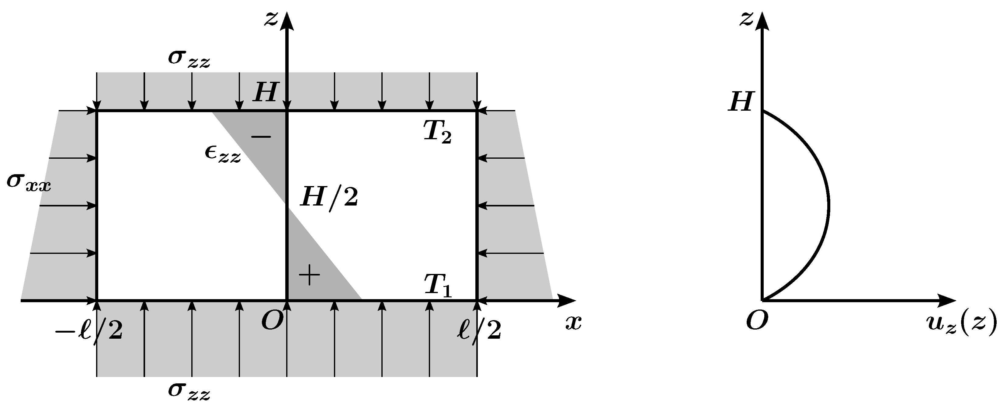
2. Problem Formulation

We consider a viscoplastic fluid filling a rigid parallelepiped container of dimensions $2\ell \times 2L\times H$ along x, y and z axes, respectively, (see Figure 1). The z-axis is directed upwards with the origin located at the bottom wall. The acceleration due to gravity reads $\mathit{g}=-g{\mathit{e}}_z$, where ${\mathit{e}}_z$ is a unit vector along z. The viscoplastic fluid is modeled as a continuous medium obeying, under the hypothesis of small transformations, a linear thermoelastic constitutive equation.

Initially, the temperature is uniform $T=T_2$ throughout the viscoplastic fluid layer. This state represents the initial configuration of the system in the sense of continuum mechanics theory. Then, the bottom wall temperature $T_1$ is slowly increased in a quasistatic manner, and the upper wall temperature is maintained at $T=T_2$. At each step, it is assumed that a temperature gradient is established under equilibrium conditions. The objective is to determine conditions for the appearance of the first signs of irreversible (plastic) flow.

For this, we express the basic thermoelastic equilibrium equations and constitutive Equation (i.e., stress–strain relationship) in terms of displacements, strains and stresses.

Subsequently, a second order ordinary differential equation for the vertical displacement is derived and solved leading to an analytical solution. Then, the stress field in the viscoplastic layer is calculated. The main yield criteria can therefore be used to determine the limit of elasticity and the onset of plastic deformation.

2.1. Governing Equations

In the framework of linear thermoelasticity [27], Cauchy’s equation of motion reads:

$$\begin{array}{c}\hfill \rho \frac{{\partial }^2\mathit{u}}{\partial t^2}=\nabla ·\mathit{\sigma }+\rho \mathit{g},\end{array}$$

(3)

with the constitutive equation

$$\begin{array}{c}\hfill \mathit{\sigma }=\lambda Tr\left(\mathit{ϵ}\right)\mathit{I}+2\mu \mathit{ϵ}-k\left(T-T_2\right)\mathit{I},\end{array}$$

(4)

where

$$\begin{array}{c}\hfill k=\left(3\lambda +2\mu \right)\alpha .\end{array}$$

(5)

In Equations (3)–(5), $\lambda$ is the elastic modulus (first Lamé’s parameter), $\mu$ is the shear modulus (second Lamé’s parameter), $\mathit{\sigma }$ is the Cauchy stress tensor, $\mathit{ϵ}$ is the strain tensor and $\mathit{u}=u_x{\mathit{e}}_x+u_y{\mathit{e}}_y+u_z{\mathit{e}}_z$ is the displacement vector. In Equation (4), it is assumed implicitly that there are no residual stresses. The strain tensor is related to the displacement gradient by the relation:

$$\begin{array}{c}\hfill \mathit{ϵ}=\frac{1}{2}\left(\nabla \mathit{u}+{(\nabla \mathit{u})}^T\right).\end{array}$$

(6)

Combining (3), (4) and (5), the problem can be written in displacement formulation (Navier equations) as:

$$\begin{array}{c}\hfill \rho \frac{{\partial }^2\mathit{u}}{\partial t^2}=\left(\lambda +\mu \right)\nabla \left(\nabla ·\mathit{u}\right)+\mu {\nabla }^2\mathit{u}+\rho \mathit{g}-k\nabla T.\end{array}$$

(7)

These equations are completed by mass and energy conservation equations:

$$\begin{array}{c}\hfill \rho ={\rho }_0\left(1-Tr\left(\mathit{ϵ}\right)\right)\end{array}$$

(8)

and

$$\begin{array}{c}\hfill \rho C_v\frac{\partial T}{\partial t}=K{\nabla }^{2}T+\mathit{\sigma }:{\dot{\mathit{ϵ}}}^p+r,\end{array}$$

(9)

where ${\rho }_0$ is the density at the reference temperature $T_2$, $C_v$ is the specific heat at constant volume, ${\dot{\mathit{ϵ}}}^p$ is the plastic strain rate, K is the thermal conductivity, and r is a possible internal heat source.

2.2. Boundary Conditions

The displacement vector $\mathit{u}$ and the temperature have to satisfy the following boundary conditions:

$$\begin{array}{ccc}& & u_x(x=\pm \ell /2,y,z)=0,\hfill \end{array}$$

(10)

$$\begin{array}{ccc}& & u_y(x,y=\pm L/2,z)=0\hfill \end{array}$$

(11)

$$\begin{array}{ccc}& & u_z(x,y,0)=u_z(x,y,H)=0\hfill \end{array}$$

(12)

$$\begin{array}{ccc}& & T(x,y,z=0)=T_1,T(x,y,z=H)=T_2\hfill \end{array}$$

(13)

$$\begin{array}{ccc}& & \frac{\partial T}{\partial x}(x=\pm \ell /2,y,z)=\frac{\partial T}{\partial y}(x,y=\pm L/2,z)=0.\hfill \end{array}$$

(14)

In the following, we consider mechanical and thermal equilibrium states such that we may drop time derivatives. We assume that there is no internal heat source in the energy equation nor irreversible deformation, i.e., ${\dot{\mathit{ϵ}}}^p=0$. The energy reduces to the uncoupled conduction equation.

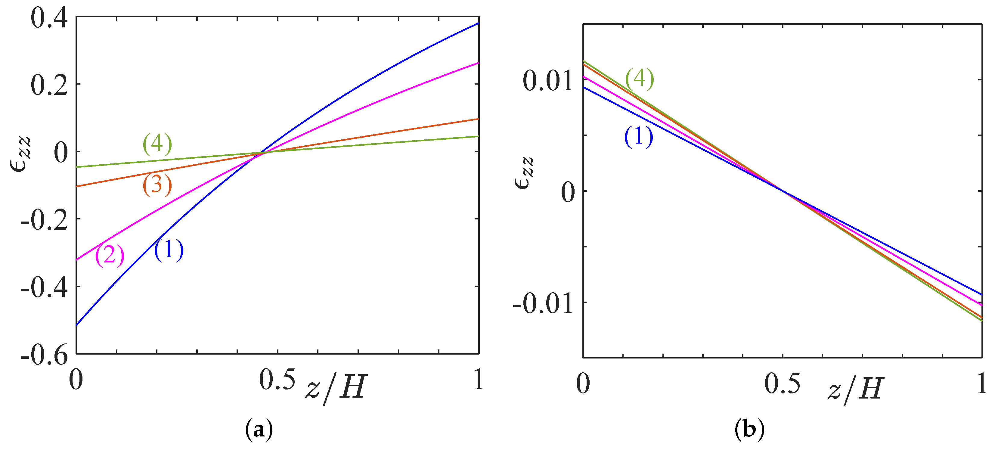
3. Thermal Stresses and Strains Induced by a Temperature Gradient

To highlight the contribution of the temperature gradient on stresses and deformations generated inside the viscoplastic fluid layer, the acceleration gravity is canceled artificially.

Sufficiently far from the lateral walls, it can be assumed that the temperature T depends only on z, with

$$\begin{array}{c}\hfill T=T_1-\mathsf{\Delta }T\frac{z}{H},\end{array}$$

(15)

where $\mathsf{\Delta }T=T_1-T_2$. The Navier equations reduce to:

$$\begin{array}{ccc}& & (\lambda +\mu )\left(\frac{{\partial }^2{u}_x}{\partial x^2}+\frac{{\partial }^2{u}_z}{\partial z\partial x}\right)+\mu \left(\frac{{\partial }^2{u}_x}{\partial x^2}+\frac{{\partial }^2{u}_x}{\partial z^2}\right)=0\hfill \end{array}$$

(16)

$$\begin{array}{ccc}& & (\lambda +\mu )\left(\frac{{\partial }^2{u}_y}{\partial y^2}+\frac{{\partial }^2{u}_z}{\partial z\partial y}\right)+\mu \left(\frac{{\partial }^2{u}_y}{\partial y^2}+\frac{{\partial }^2{u}_y}{\partial z^2}\right)=0\hfill \end{array}$$

(17)

$$\begin{array}{ccc}& & (\lambda +\mu )\left(\frac{{\partial }^2{u}_x}{\partial x\partial z}+\frac{{\partial }^2{u}_y}{\partial y\partial z}+\frac{{\partial }^2{u}_z}{\partial z^2}\right)+\mu \left(\frac{{\partial }^2{u}_z}{\partial x^2}+\frac{{\partial }^2{u}_z}{\partial y^2}+\frac{{\partial }^2{u}_z}{\partial z^2}\right)+\frac{k(T_1-T_2)}{H}=0.\hfill \end{array}$$

(18)

To obtain an analytical solution, we consider, as a first approach, a solution that satisfies the boundary conditions and depends only on z. By doing this, we suppose implicitly that the aspect ratio $\ell /H$ is large. Based on these assumptions, the solution of the Navier equations leads to the following expression of the displacement:

$$\begin{array}{c}\hfill \mathit{u}=\frac{\chi }{2}z(1-\frac{z}{H}){\mathit{e}}_z,\end{array}$$

(19)

where,

$$\begin{array}{c}\hfill \chi =\frac{k\mathsf{\Delta }T}{\lambda +2\mu }\end{array}$$

(20)

accounts for the uniaxial deformation due to thermal stresses. The strain-tensor is then given by

$$\begin{array}{c}\hfill \mathit{ϵ}=\chi \left(\frac{1}{2}-\frac{z}{H}\right){\mathit{e}}_z\otimes {\mathit{e}}_z.\end{array}$$

(21)

${ϵ}_{zz}$ is positive for $0<z<H/2$ and negative for $H/2<z<H$ as illustrated in Figure 1. The gel undergoes an expansion near the heated wall, between 0 and $H/2$ and a compression near the cooled wall, between $H/2$ and H. The gel layer is therefore subjected to thermal stresses. They are determined by substituting (21) into the constitutive Equation (4). We obtain:

$$\begin{array}{ccc}& & {\sigma }_{xx}={\sigma }_{yy}=\chi \left(2\mu \frac{z}{H}-\frac{\lambda +4\mu }{2}\right),\hfill \end{array}$$

(22)

$$\begin{array}{ccc}& & {\sigma }_{zz}=-\frac{1}{2}k\mathsf{\Delta }T,\hfill \end{array}$$

(23)

$$\begin{array}{ccc}& & {\sigma }_{ij}=0\mathrm{if}i\ne j.\hfill \end{array}$$

(24)

Given the well known relationships between the Lamé parameters, Young’s modulus E and Poisson’s ratio $\nu$,

$$\begin{array}{c}\hfill \lambda =\frac{E\nu }{\left(1-2\nu \right)\left(1+\nu \right)}\mathrm{and}\mu =\frac{E}{2\left(1+\nu \right)},\end{array}$$

(25)

it can be shown straightforwardly that, for an incompressible elastic material, where $\nu =1/2$, one recovers the state of the hydrostatic pressure

$$\begin{array}{c}\hfill {\sigma }_{xx}={\sigma }_{yy}={\sigma }_{zz}=-\frac{k}{2}\mathsf{\Delta }T.\end{array}$$

(26)

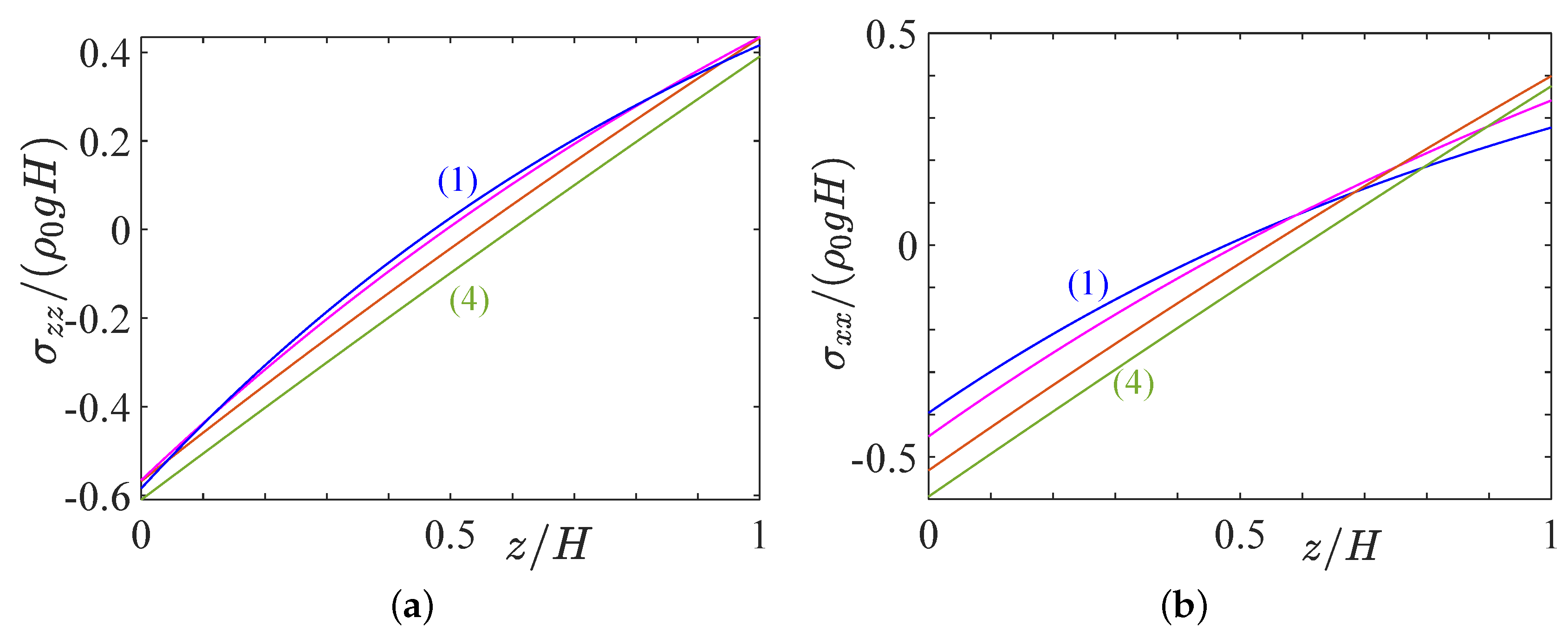
4. Strain and Stress Fields Induced by Gravity Combined with a Temperature Gradient

As indicated previously, for small deformations, the mass conservation equation reduces to

$$\begin{array}{c}\hfill \rho \left(z\right)={\rho }_0\left(1-{ϵ}_{zz}\right)\approx {\rho }_0\left(1-\frac{\partial u_z}{\partial z}\right)\end{array}$$

(27)

Substituting expression (27) into Equation (7), we obtain, for the z-component of the Navier equations,

$$\begin{array}{c}\hfill \left(\lambda +2\mu \right)\frac{{\partial }^2{u}_z}{\partial z^2}+\frac{k\mathsf{\Delta }T}{H}-{\rho }_{0}g\left(1-\frac{\partial u_z}{\partial z}\right)=0,\end{array}$$

(28)

with the boundary conditions

$$\begin{array}{c}\hfill u_z=0\mathrm{at}z=0,H.\end{array}$$

(29)

The solution $u_z$ is then given by

$$\begin{array}{c}\hfill {\displaystyle u_z\left(z\right)=\left(1-\kappa \right)\left(\frac{z}{H}-\frac{1-exp\left(-\frac{1}{\mathsf{\Lambda }}\frac{z}{H}\right)}{1-exp\left(-\frac{1}{\mathsf{\Lambda }}\right)}\right)H,}\end{array}$$

(30)

and the only non-zero component of the deformation tensor is

$$\begin{array}{c}\hfill {\displaystyle {ϵ}_{zz}\left(z\right)=(1-\kappa )\left(1-\frac{1}{\mathsf{\Lambda }}\frac{exp\left(-\frac{z}{\mathsf{\Lambda }H}\right)}{1-exp\left(-\frac{1}{\mathsf{\Lambda }}\right)}\right).}\end{array}$$

(31)

The dimensionless parameter $\kappa$ defined by

$$\begin{array}{c}\hfill {\displaystyle \kappa =\frac{k\mathsf{\Delta }T}{{\rho }_{0}gH}}\end{array}$$

(32)

is the ratio of thermal stresses to gravitational stresses, and

$$\begin{array}{c}\hfill {\displaystyle \frac{1}{\mathsf{\Lambda }}=\frac{{\rho }_{0}gH}{\lambda +2\mu }}\end{array}$$

(33)

represents the uniaxial deformation due to gravitational stresses.

The components of the stress tensor are obtained by using the linear thermoelastic constitutive equation:

$$\begin{array}{ccc}\hfill {\displaystyle }& & {\sigma }_{xx}\left(z\right)=(1-\kappa )\left[\frac{3\mathsf{\Psi }-\mathsf{\Lambda }}{2}\left(1-\frac{1}{\mathsf{\Lambda }}\frac{exp\left(-\frac{z}{\mathsf{\Lambda }H}\right)}{1-exp\left(-\frac{1}{\mathsf{\Lambda }}\right)}\right)-\frac{\kappa }{1-\kappa }\left(1-\frac{z}{H}\right)\right]{\rho }_{0}gH,\hfill \end{array}$$

(34)

$$\begin{array}{ccc}& & {\displaystyle {\sigma }_{yy}\left(z\right)={\sigma }_{xx}\left(z\right),}\hfill \end{array}$$

(35)

$$\begin{array}{ccc}& & {\displaystyle {\sigma }_{zz}\left(z\right)=(1-\kappa )\left[\mathsf{\Lambda }\left(1-\frac{1}{\mathsf{\Lambda }}\frac{exp\left(-\frac{z}{\mathsf{\Lambda }H}\right)}{1-exp\left(-\frac{1}{\mathsf{\Lambda }}\right)}\right)-\frac{\kappa }{1-\kappa }\left(1-\frac{z}{H}\right)\right]{\rho }_{0}gH}\hfill \end{array}$$

(36)

where

$$\begin{array}{c}\hfill \mathsf{\Psi }=\frac{3\lambda +2\mu }{3{\rho }_{0}gH}\end{array}$$

(37)

The hydrostatic pressure ${\displaystyle p=(1/3)Tr\left(\mathit{ϵ}\right)}$ is then

$$\begin{array}{c}\hfill {\displaystyle p=(1-\kappa )\left[\mathsf{\Psi }\left(1-\frac{1}{\mathsf{\Lambda }}\frac{exp\left(-\frac{z}{\mathsf{\Lambda }H}\right)}{1-exp\left(-\frac{1}{\mathsf{\Lambda }}\right)}\right)-\frac{\kappa }{1-\kappa }\left(1-\frac{z}{H}\right)\right]{\rho }_{0}gH}\end{array}$$

(38)

The dimensionless parameter $1/\mathsf{\Psi }$ accounts for the volume variation induced by gravitational stresses.

In Figure 2a, we represent the deformation ${ϵ}_{zz}$ as a function of the dimensionless vertical position $z/H$ for different values of $\kappa$, $\mathsf{\Lambda }$ and $\mathsf{\Psi }$. Two situations are considered: (a) ${ϵ}_{zz}$ induced by the gravity combined with a temperature gradient and (b) ${ϵ}_{zz}$ induced only by a temperature gradient. The $\kappa$ and $\mathsf{\Lambda }$ values have been determined by considering a gel layer with the following properties: $H=0.02\mathrm{m}$, $\rho ={10}^3\mathrm{k}\mathrm{g}/{\mathrm{m}}^3$, $E=100\mathrm{Pa}$, $\alpha =2\times {10}^{-4}{\mathrm{K}}^{-1}$ and $\nu =0.4,0.44,0.48$ and $0.49$. The temperature difference was fixed to $\mathsf{\Delta }T=40$ ${}^{°}$C.

We note that: (i) The gravity effect is much more significant than that induced by the temperature gradient. (ii) These two effects act in opposite ways. Hence, in the lower part of the gel layer, the gravity induces a compression while the temperature gradient induces an expansion and vice versa in the upper part. (iii) With increasing $\mathsf{\Lambda }$ and $\mathsf{\Psi }$, the strain ${ϵ}_{zz}$ decreases. The resulting stress field in the gel layer is illustrated through the components ${\sigma }_{zz}$ and ${\sigma }_{xx}$ represented as a function of $z/H$ in Figure 3. ${\sigma }_{zz}$ and ${\sigma }_{xx}$ are of the same order.

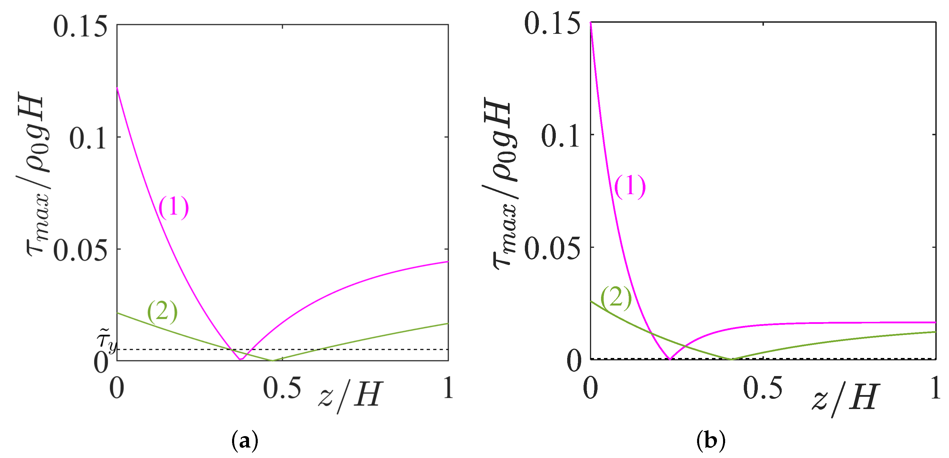
5. Onset of Plastic Deformation: Main Yield Criteria

A number of yield criteria have been developed in the literature to determine the limit of elasticity and the onset of plastic deformation. In this section, three criteria of yielding—namely, the criteria of Tresca, von Mises and Drucker–Prager—are considered.

5.1. Tresca Criterion

From Mohr’s circle, it can be shown straightforwardly that the maximum of shear-stress ${\tau }_{max}$ at any point in the gel layer is given by:

$$\begin{array}{c}\hfill {\tau }_{max}=\frac{\left|{\sigma }_{xx}-{\sigma }_{zz}\right|}{2}=\mu \left|{ϵ}_{zz}\right|.\end{array}$$

(39)

In dimensionless form, we have

$$\begin{array}{c}\hfill \frac{{\tau }_{max}}{{\rho }_{0}gH}=\frac{3}{4}\left|\mathsf{\Lambda }-\mathsf{\Psi }\right|\left|1-\kappa \right|\left|1-\frac{1}{\mathsf{\Lambda }}\frac{exp\left(-\frac{z}{\mathsf{\Lambda }H}\right)}{1-exp\left(-\frac{1}{\mathsf{\Lambda }}\right)}\right|.\end{array}$$

(40)

According to the Tresca criterion, the onset of plastic yielding is defined by the condition:

$$\begin{array}{c}\hfill {\tau }_{max}={\tau }_y,\end{array}$$

(41)

where ${\tau }_y$ is the shear yield stress. The variation of ${\tau }_{max}/{\rho }_{0}gH$ as a function of the dimensionless vertical position $z/H$ is depicted in Figure 4a for different values of the dimensionless parameters $\kappa ,\mathsf{\Lambda }$ and $\mathsf{\Psi }$. Curves (1), (2) and (3) with the associated dimensionless parameters were obtained for three values of the Poisson’s ratio $\nu =0.4,0.44$ and $0.48$, respectively, and by setting $E=100\mathrm{Pa}$, $H=0.02\mathrm{m}$, ${\rho }_0={10}^3\mathrm{k}\mathrm{g}/{\mathrm{m}}^3$, $\mathsf{\Delta }T=40 °\mathrm{C}$, $\alpha =2\times {10}^{-4}{K}^{-1}$. The maximum shear-stress decreases with increasing $\mathsf{\Lambda }$ and $\mathsf{\Psi }$, i.e., by increasing, for instance, the Poisson’s ratio.

Figure 4a shows that the yielding in the gel layer starts when the yield shear stress ${\tau }_y$ is smaller than ${\tau }_{max}(z=0)$. In Figure 4b, the thermal effects are canceled by setting $\mathsf{\Delta }T=0$. Comparatively to Figure 4a, the curves (1), (2) and (3) are slightly modified. ${\tau }_{max}/{\rho }_{0}gH$ actually decreases slightly in the presence of thermal effects. Indeed, for the rheological parameters considered here, the thermal effects are much weaker than gravitational effects and act in opposite ways on the strain and stress fields in the gel layer. In other words, if, for $\mathsf{\Delta }T=0$, ${\tau }_{max}<{\tau }_y$, then the gel layer will remain in the elastic domain when the temperature difference between the top and bottom walls increases within a reasonable range.

The application of Tresca criterion to experiments of Kebiche et al. [13] is shown in Figure 5a. The experimental parameters are $H=0.02\mathrm{m}$, $\rho ={10}^3\mathrm{k}\mathrm{g}/{\mathrm{m}}^3$, $\mu =10\mathrm{Pa},\alpha =2\times {10}^{-4}{\mathrm{K}}^{-1}$ and ${\tau }_y=1\mathrm{Pa}$. The onset of convection was observed at $\mathsf{\Delta }T\approx 8°\mathrm{C}$. As the Poisson’s ratio is not given, we used two values $\nu =0.4$ and $0.48$. This leads to two triplets $(\kappa ,\mathsf{\Lambda },\mathsf{\Psi })$: ($1.14\times {10}^{-3},0.306,0.238$) curve 1 and $(6.03\times {10}^{-3},1.325,1.257)$ curve 2. Again, the low values of $\kappa$ indicate that the thermal effects are negligible. Indeed, curves 1 and 2 are almost unchanged if one sets $\mathsf{\Delta }T=0$.

The figure clearly shows that, at the beginning of the experiment, i.e., at $\mathsf{\Delta }T=0$, in a large part of the Carbopol gel layer, ${\tau }_{max}/{\rho }_{0}gH>{\tau }_y/{\rho }_{0}gH$, i.e., the material has already crossed the threshold of plasticity. In the experiments of Darbouli et al. [12], where $H=0.02\mathrm{m}$, ${\tau }_y=0.1\mathrm{Pa}$, $\mu =3.25\mathrm{Pa},\alpha =7.4\times {10}^{-5}{\mathrm{K}}^{-1}$ and $\mathsf{\Delta }T\approx 50°\mathrm{C}$, the whole gel layer is yielded. Indeed, the limit ${\tau }_y/{\rho }_{0}gH=5.09\times {10}^{-4}$ almost coincides with the abscissa axis.

5.2. Von Mises Yield Criterion

The von Mises yield criterion suggests that the yielding of materials begins when the second deviatoric stress invariant $J_2$ reaches a critical value. This condition is represented by the equation

$$\begin{array}{c}\hfill \sqrt{3J_2}={\sigma }_y,\end{array}$$

(42)

where ${\sigma }_y$ is a tensile yield strength of the material. At the onset of yielding, the magnitude of shear yield stress in pure shear is $\sqrt{3}$-times lower than the tensile yield stress. The von Mises criterion can be viewed as a particular case of the Drucker–Prager criterion. The analysis of these criteria is done in the following section.

5.3. Drucker–Prager Yield Criterion

The Drucker–Prager yield criterion is a modification of the von Mises criterion, whereby the hydrostatic pressure-dependent first invariant $I_1$ is introduced. It can be expressed as

$$\begin{array}{c}\hfill \sqrt{3J_2}+A\left|I_1\right|={\sigma }_y,\end{array}$$

(43)

where $I_1$ is the first invariant of Cauchy stress tensor and A a material parameter. The following expressions are obtained for $\sqrt{3J_2}$ and $I_1$:

$$\begin{array}{ccc}& & {\displaystyle \sqrt{3J_2}=\left|{\sigma }_{xx}-{\sigma }_{zz}\right|=\frac{3}{2}\left|\left(\mathsf{\Lambda }-\mathsf{\Psi }\right)(1-\kappa )\left(1-\frac{1}{\mathsf{\Lambda }}\frac{exp\left(-\frac{z}{H\mathsf{\Lambda }}\right)}{1-exp\left(-\frac{1}{\mathsf{\Lambda }}\right)}\right)\right|{\rho }_{0}gH,}\hfill \end{array}$$

(44)

$$\begin{array}{ccc}& & {\displaystyle I_1=\frac{1}{3}Tr\left(\mathit{\sigma }\right)=\mathsf{\Psi }\left(1-\kappa \right)\left(1-\frac{1}{\mathsf{\Lambda }}\frac{exp\left(-\frac{z}{H\mathsf{\Lambda }}\right)}{1-exp\left(-\frac{1}{\mathsf{\Lambda }}\right)}\right){\rho }_{0}gH-\kappa \left(1-\frac{z}{H}\right){\rho }_{0}gH}\hfill \end{array}$$

(45)

In Figure 6a, we represented the values of the couple $\left(\sqrt{3J_2}/{\rho }_{0}gH,\left|I_1\right|/{\rho }_{0}gH\right)$ at different vertical positions $z/H$ and for different values of the dimensionless parameters $\kappa$, $\mathsf{\Lambda }$ and $\mathsf{\Psi }$. We used the same values of the dimensionless parameters $\kappa$, $\mathsf{\Lambda }$ and $\mathsf{\Psi }$ as in Figure 4a. The curves have a U shape. The lowest value of $\left|{\sigma }_{zz}-{\sigma }_{xx}\right|$ is reached at the central part of the gel layer.

The Drucker–Prager yield criterion is represented by setting ${\sigma }_y=10\sqrt{3}\mathrm{Pa}$ and two values of A: $0.05$ and $0.2$. The von Mises yield criterion corresponds to $A=0$. Below the lines representing the yield criterion, the material behaves as an elastic solid. Above, the material enters the plastic domain. Depending on the experimental conditions, the gel in the central area may be in the elastic domain, whereas outside, it has already entered the plastic domain. By increasing $\mathsf{\Lambda }$ and $\mathsf{\Psi }$, i.e., the elastic effects, we increase the central zone where the material remains elastic. By increasing the influence of the hydrostatic pressure in the yield criterion, i.e., by increasing A, the onset of yielding in precipitated.

In Figure 6b, the thermal effects are canceled by setting $\kappa =0$, and the extent of the elastic or the plastic zone is not significantly modified comparatively to Figure 6a. The numerical results show a very slight increase of the elastic zone. In addition, the two branches of the U shape have merged.

The application of the Drucker–Prager criterion to experiments of Kebiche et al. [13] and Darbouli et al. [12] is illustrated in Figure 7a,b. In both cases, the thermal effects are very small compared to the gravity effects. By setting $\mathsf{\Delta }T=0$, the curves are almost not modified. It can be noted for Figure 7b, that almost all the gel layer has entered the plastic domain by gravity effects only.

6. Conclusions

Using the linear theory of thermoelasticity, we derived an analytical solution for stresses and strains generated in a layer of a viscoplastic fluid confined in a parallelepiped box. The analysis shows that the problem is governed by three dimensionless groups denoted as $\kappa ,\mathsf{\Lambda }$ and $\mathsf{\Psi }$, where $\kappa$ is the ratio between thermal and gravitational stresses and $1/\mathsf{\Lambda }$ and $1/\mathsf{\Psi }$ account for uniaxial deformation and volume variation, respectively, due to gravitational stresses.

We demonstrated that gravity and the thermal gradient have antagonistic effects. Indeed, gravity generates a compression at the lower part of the gel layer, whereas a thermal gradient (the layer is heated from the bottom) generates an expansion in the lower part of the gel layer. However, within the range of the rheological and geometrical parameters considered and for a reasonable temperature difference, the thermal effects were much weaker than the gravitational effects. The onset of yielding was then investigated using the classical yield criteria (Tresca, von Mises and Drucker–Prager). We found that, in the experiments of Kebiche et al. [13], a large part of the gel layer was yielded, whereas, in Darbouli et al. [12], almost all the gel layer was yielded. In these experiments, $\kappa =\mathrm{O}\left({10}^{-3}\right)$, i.e., the thermal stresses were ${10}^3$-times weaker than the gravitational ones.

When the stress state enters the plastic regime due to an increase in thermomechanical stresses (imposed by the temperature gradient and the gravitation), plastic flow occurs with a specific distribution of displacements, strains and stresses. In our future work, we intend to investigate more general equilibrium states of the gel and to analyze more thoroughly the onset of yielding and the beginning of the plastic flow process. A simple model will be considered assuming that the thermoelastoplastic behavior of the medium is independent of the strain rate.

References

1. Balmforth, N.; Frigaard, I.; Ovarlez, G. Yielding to stress: Recent developments in viscoplastic fluid mechanics. Annu. Rev. Fluid Mech. 2014, 46, 121–146. [Google Scholar] [CrossRef]
2. Coussot, P. Bingham’s heritage. Rheol. Acta 2017, 56, 163–176. [Google Scholar] [CrossRef]
3. Bonn, D.; Denn, M.; Berthier, L.; Divoux, T.; Manneville, S. Yield stress materials in soft condensed matter. Rev. Mod. Phys. 2017, 89, 035005. [Google Scholar] [CrossRef] [Green Version]
4. Zhang, J.; Vola, D.; Frigaard, I. Yield stress effects on Rayleigh–Bénard convection. J. Fluid Mech. 2006, 566, 389–419. [Google Scholar] [CrossRef]
5. Balmforth, N.; Rust, A. Weakly nonlinear viscoplastic convection. J. Non–Newton. Fluid Mech. 2009, 158, 36–45. [Google Scholar] [CrossRef]
6. Vikhansky, A. Thermal convection of a viscoplastic liquid with high Rayleigh and Bingham numbers. Phys. Fluids 2009, 21, 103103. [Google Scholar] [CrossRef]
7. Turan, O.; Poole, R.; Chakraborty, N. Influences of boundary conditions on laminar natural convection in rectangular enclosures with differentially heated side walls. Int. J. Heat Fluid Flow 2012, 33, 131–146. [Google Scholar] [CrossRef]
8. Turan, O.; Yigit, S.; Chakraborty, N. Critical condition for Rayleigh-Bénard convection of Bingham fluids in rectangular enclosures. Int. Commun. Heat Mass Transf. 2017, 86, 117–125. [Google Scholar] [CrossRef] [Green Version]
9. Aghighi, M.; Ammar, A.; Masoumi, H.; Lanjabi, A. Rayleigh–Bénard convection of a viscoplastic liquid in a trapezoidal enclosure. Int. J. Mech. Sci. 2020, 180, 105630. [Google Scholar] [CrossRef]
10. Aghighi, M.; Ammar, A. Aspect ratio effects in Rayleigh–Bénard convection of Herschel–Bulkley fluids. Eng. Comput. 2017. [Google Scholar] [CrossRef]
11. Aghighi, M.; Ammar, A.; Metivier, C.; Gharagozlu, M. Rayleigh-Bénard convection of Casson fluids. Int. J. Therm. Sci. 2018, 127, 79–90. [Google Scholar] [CrossRef] [Green Version]
12. Darbouli, M.; Métivier, C.; Piau, J.M.; Magnin, A.; Abdelali, A. Rayleigh-Bénard convection for viscoplastic fluids. Phys. Fluids 2013, 25, 023101. [Google Scholar] [CrossRef] [Green Version]
13. Kebiche, Z.; Castelain, C.; Burghelea, T. Experimental investigation of the Rayleigh–Bénard convection in a yield stress fluid. J. Non–Newton. Fluid Mech. 2014, 203, 9–23. [Google Scholar] [CrossRef]
14. Hurle, D.; Jakeman, E.; Pike, E. On the solution of the Bénard problem with boundaries of finite conductivity. Proc. R. Soc. Lond. A Math Phys. Sci. 1967, 296, 469–475. [Google Scholar]
15. Piau, J. Carbopol gels: Elastoviscoplastic and slippery glasses made of individual swollen sponges: Meso-and macroscopic properties, constitutive equations and scaling laws. J. Non–Newton. Fluid Mech. 2007, 144, 1–29. [Google Scholar] [CrossRef]
16. Cloitre, M.; Bonnecaze, R. A review on wall slip in high solid dispersions. Rheol. Acta 2017, 56, 283–305. [Google Scholar] [CrossRef]
17. Cerisier, P.; Rahal, S.; Cordonnier, J.; Lebon, G. Thermal influence of boundaries on the onset of Rayleigh-Bénard convection. Int. J. Heat Mass Transf. 1998, 41, 3309–3320. [Google Scholar] [CrossRef]
18. Bouteraa, M.; Nouar, C.; Plaut, E.; Métivier, C.; Kalck, A. Weakly nonlinear analysis of Rayleigh-Bénard convection in shear-thinning fluids: Nature of the bifurcation and pattern selection. J. Fluid. Mech 2015, 767, 696–734. [Google Scholar] [CrossRef]
19. Davaille, A.; Gueslin, B.; Massmeyer, A.; Giuseppe, E.D. Thermal instabilities in a yield stress fluid: Existence and morphology. J. Non–Newton. Fluid Mech. 2013, 193, 144–153. [Google Scholar] [CrossRef]
20. Jadhav, K.; Rossi, P.; Karimfazli, I. Motion onset in simple yield stress fluids. J. Fluid Mech. 2021, 912. [Google Scholar] [CrossRef]
21. Ahmadi, A.; Olleik, H.; Karimfazli, I. Rayleigh–Bénard convection of carbopol microgels: Are viscoplastic models adequate? J. Non–Newton. Fluid Mech. 2022, 300, 104704. [Google Scholar] [CrossRef]
22. Metivier, C.; Li, C.; Magnin, A. Origin of the onset of Rayleigh-Bénard convection in a concentrated suspension of microgels with a yield stress behavior. Phys. Fluids 2017, 29, 104102. [Google Scholar] [CrossRef] [Green Version]
23. Horton, C.; Rogers, J. Convection currents in a porous medium. J. Appl. Phys. 1945, 16, 367–370. [Google Scholar] [CrossRef]
24. Lapwood, E. Convection of a fluid in a porous medium. In Mathematical Proceedings of the Cambridge Philosophical Society; Cambridge University Press: Cambridge, MA, USA, 1948; Volume 44, pp. 508–521. [Google Scholar]
25. Nield, D.A.; Bejan, A. Convection in Porous Media; Springer: Berlin/Heidelberg, Germany, 2006; Volume 3. [Google Scholar]
26. Tiu, C.; Guo, J.; Uhlherr, P.; Heinz, T. Yielding behaviour of viscoplastic materials. J. Ind. Eng. Chem. 2006, 12, 653–662. [Google Scholar]
27. Salençon, J. Mécanique des Milieux Continus: Thermoélasticité Linéaire; Editions Ecole Polytechnique: Paris, France, 2000; Volume 2. [Google Scholar]
Figure 1. Illustration of the strain ϵ z z , stress σ and displacement u z induced by a temperature gradient.
Fluids 07 00231 g001
Figure 2. (a) Illustration of the strain ϵ z z induced by the gravity combined with a temperature gradient for different values of κ , Λ and Ψ : (1) κ , Λ , Ψ = ( 0.0204 , 1.092 , 0.849 ) , (2) ( 0.0340 , 1.652 , 1.416 ) , (3) ( 0.102 , 4.477 , 4.247 ) , (4) ( 0.204 , 8.723 , 8.495 ) . (b) The strain ϵ z z induced only by a temperature gradient. (1) χ = 0.0187 , (2) χ = 0.0206 , (3) χ = 0.0228 and (4) χ = 0.0234 .
Fluids 07 00231 g002
Figure 3. Illustration of stresses (a) σ z z and (b) σ x x induced by gravity combined with a temperature gradient. (1) κ , Λ , Ψ = ( 0.0204 , 1.092 , 0.849 ) , (2) ( 0.0340 , 1.652 , 1.416 ) , (3) ( 0.102 , 4.477 , 4.247 ) and (4) ( 0.204 , 8.723 , 8.495 ) .
Fluids 07 00231 g003
Figure 4. Variation of τ m a x / ρ 0 g H as a function of z / H for different triplets ( κ , Λ , Ψ ) . (a) (1): ( 0.0204 , 1.092 , 0.849 ) , (2) ( 0.0340 , 1.652 , 1.416 ) and (3): ( 0.102 , 4.477 , 4.247 ) . (b) Same parameters Λ and Ψ with κ = 0 .
Fluids 07 00231 g004
Figure 5. Variation of τ m a x / ρ 0 g H as a function of z / H . (a) Experiments of Kebiche et al. [13] where τ ˜ y = τ y / ρ 0 g H = 5.09 × 10 3 : (1) κ = 1.14 × 10 3 , Λ = 0.306 , Ψ = 0.238 , (2) κ = 6.03 × 10 3 , Λ = 1.325 , Ψ = 1.257 . (b) Experiments of Darbouli et al. [12]: (1) κ = 8.58 × 10 4 , Λ = 9.94 × 10 2 , Ψ = 7.73 × 10 2 , (2) κ = 4.53 × 10 3 , Λ = 0.431 , Ψ = 0.409 . The dashed line corresponding to τ y / ρ 0 g H = 5.09 × 10 4 almost coincides with the x-axis.
Fluids 07 00231 g005
Figure 6. Values of the couple 3 J 2 / ρ 0 g H , | I 1 | / ρ 0 g H at different vertical positions and for different triplets ( κ , Λ , Ψ ) . (a) (1): ( 0.0204 , 1.092 , 0.849 ) , (2): ( 0.0340 , 1.652 , 1.416 ) , and (3): ( 0.102 , 4.477 , 4.247 ) . (b) The same parameters Λ and Ψ as in (a) with κ = 0 . (4): (dashed line) Drucker–Prager criterion for A = 0.05 , and (5): (dashed line) Drucker–Prager criterion for A = 0.2 . The horizontal dashed line ( A = 0 ) is the von Mises yield criterion with σ y = 10 3 .
Fluids 07 00231 g006
Figure 7. Values of the couple 3 J 2 / ρ 0 g H , | I 1 | / ρ 0 g H at different vertical positions. (a) Experiments of Kebiche et al. [13]: (1) κ = 1.14 × 10 3 , Λ = 0.306 , Ψ = 0.238 , (2) κ = 6.03 × 10 3 , Λ = 1.325 , Ψ = 1.257 , σ y / ρ 0 g H = 8.83 × 10 3 . The dashed line is the Drucker–Prager criterion for A = 0.1 , and the horizontal line is the von Mises criterion ( A = 0 ). (b) Experiments of Darbouli et al. [12]: (1) κ = 8.58 × 10 4 , Λ = 9.94 × 10 2 , Ψ = 7.73 × 10 2 , and (2) κ = 4.53 × 10 3 , Λ = 0.431 , Ψ = 0.409 , σ y / ρ 0 g H = 8.83 × 10 4 .
Fluids 07 00231 g007
Publisher’s Note: MDPI stays neutral with regard to jurisdictional claims in published maps and institutional affiliations.