
Prediction of Critical Heat Flux for Subcooled Flow Boiling in Annulus and Transient Surface Temperature Change at CHF

Abstract
:1. Introduction
2. Liquid Sublayer Dryout Model and Its Application to an Annulus
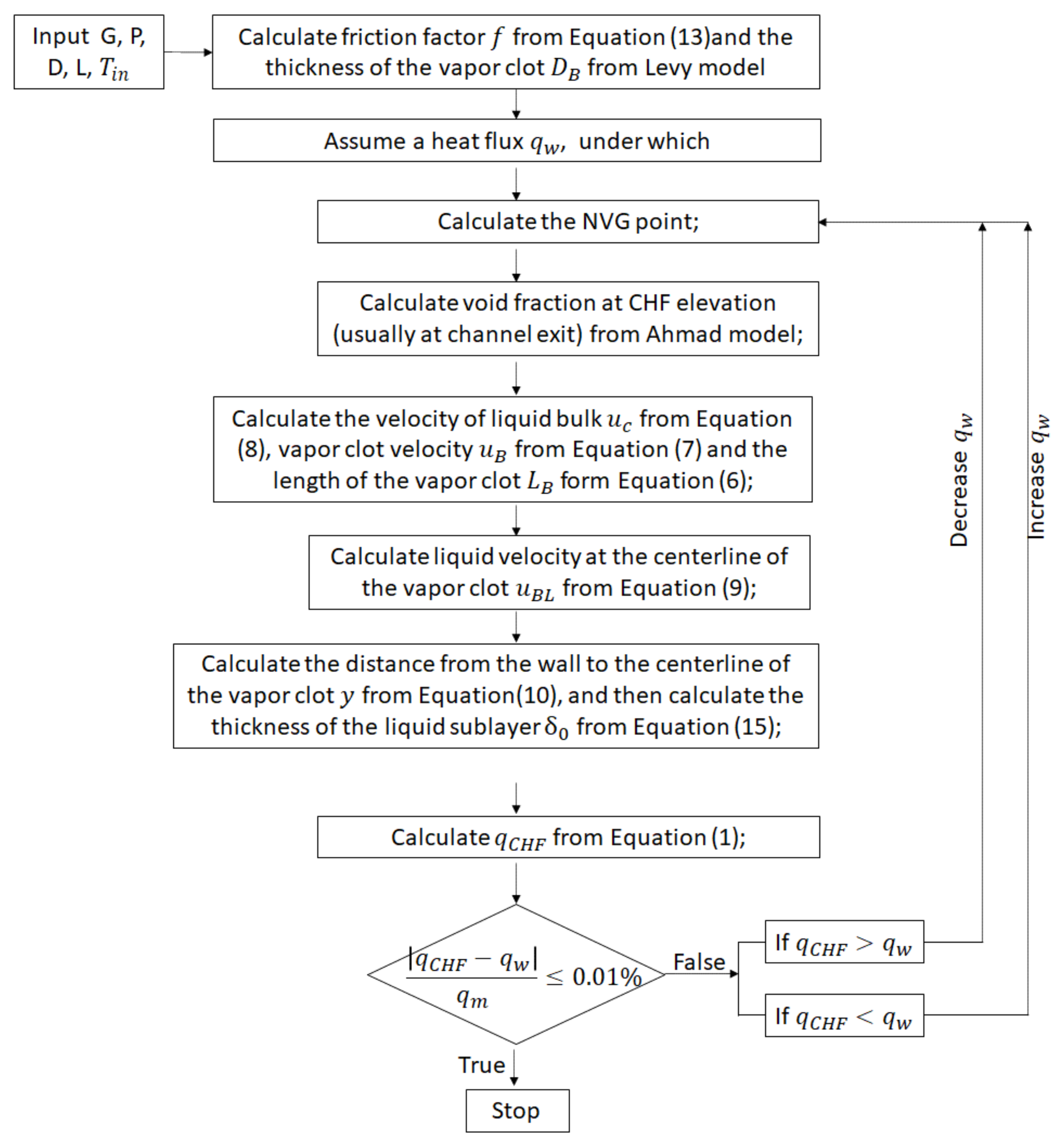
3. Prediction of CHF in an Annulus
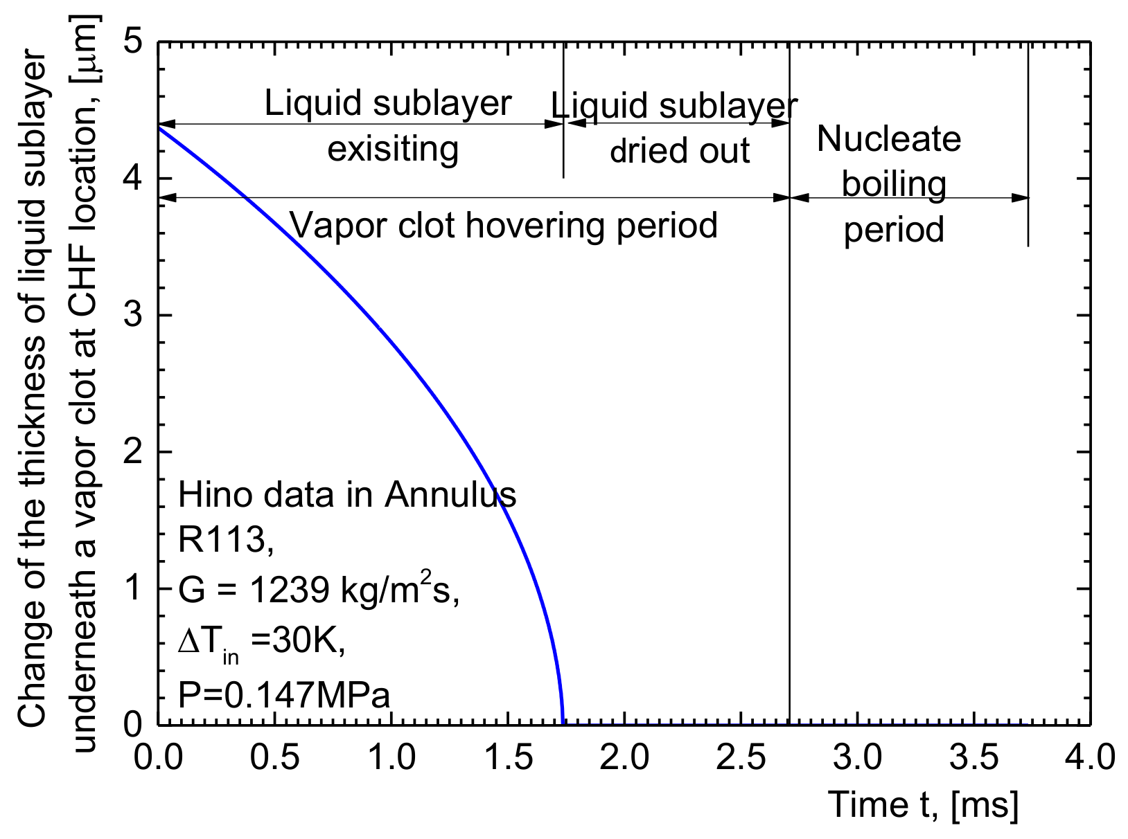
4. Predictions of the Changes in Liquid Sublayer Thickness and Heater Surface Temperature at the CHF
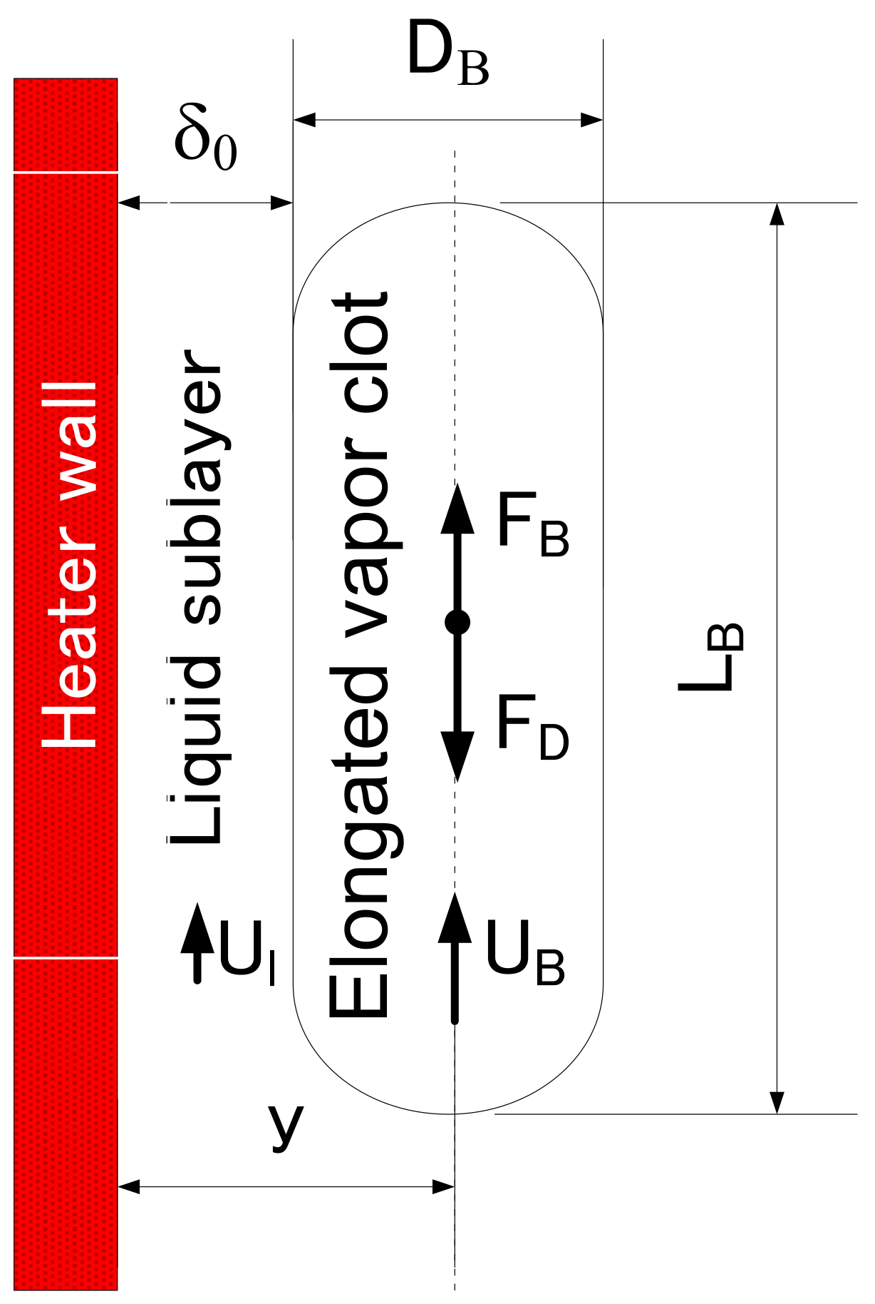
4.1. Modeling of Near Wall Vapor–Liquid Structure at the CHF
4.2. Modeling of Heat Transfer Modes over Heated Surface near the CHF
4.3. Analysis Case
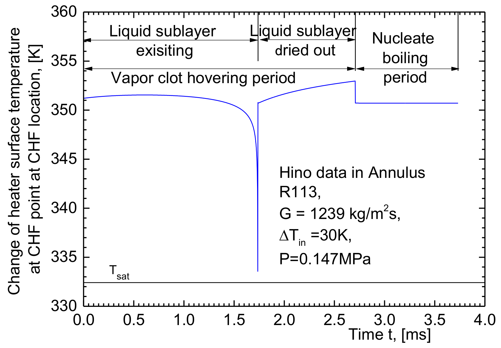
4.4. Calculation of Transient Heater Surface Temperature Change at CHF
5. Concluding Remarks
Author Contributions
Funding
Institutional Review Board Statement
Informed Consent Statement
Data Availability Statement
Conflicts of Interest
Nomenclature
| Latin symbols: | |
| ratio of the area where boiling occurs on the heating surface, dimensionless | |
| coefficient in Equation (3) | |
| drag coefficient, dimensionless | |
| specific heat of the heater, ] | |
| equivalent diameter of test section, [m] | |
| thickness of the vapor clot, [] | |
| friction factor, dimensionless | |
| buoyancy force, [N] | |
| drag force, [N] | |
| G | mass flux, [] |
| heat transfer coefficient in liquid single-phase flow, [] | |
| heat transfer coefficient of liquid, [] | |
| latent heat, [] | |
| heat transfer coefficient of vapor steam, [] | |
| thermal conductivity of the heater, [] | |
| thermal conductivity of the liquid sublayer, [] | |
| thermal conductivity of the vapor, [] | |
| heating length of test section, [m] | |
| length of the elongated vapor clot, [] | |
| region where the liquid sublayer has been completely evaporated under the vapor clot, [] | |
| region where the liquid sublayer presents under the vapor clot, [] | |
| length of nucleate boiling region, [] | |
| NVG | net vapor generation point |
| P | system pressure, [] |
| heat flux transferred by liquid single-phase, [] | |
| heat flux transferred by boiling, [] | |
| calculated CHF, [] | |
| wall surface heat flux, [] | |
| volumetric heating density, [] | |
| Reynolds number, dimensionless | |
| radius direction in heat conduction equation in cylindrical coordinate, [] | |
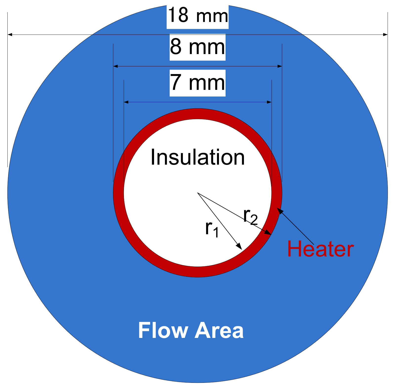
| heater inner radius in Figure 4, [] | |
| heater outer radius, and the inner radius of annulus flow channel, as shown in Figure 4, [] | |
| heater temperature, [] | |
| liquid temperature at the inlet of test section, [] | |
| steam vapor temperature, [] | |
| saturation temperature, [] | |
| wall temperature at the heater surface, [] | |
| time, [] | |
| velocity of the vapor clot, [] | |
| average velocity of liquid bulk, [] | |
| liquid velocity at the centerline of the vapor clot, [] | |
| velocity profile inside liquid phase, [m/s] | |
| velocity of the liquid sublayer, [] | |
| dimensionless velocity in liquid phase | |
| friction velocity, [] | |
| distance form heated wall to the centerline of vapor clot, [m] | |
| dimensionless distance from heated wall | |
| Greek Symbols: | |
| void fraction, dimensionless | |
| initial thickness of liquid sublayer, [] | |
| δ | thickness of the liquid sublayer, [] |
| Helmholz instability wavelength at the interface between the liquid sublayer, [] | |
| Helmholz instability wavelength at the interface between vapor clot and liquid bulk, [] | |
| subcooling of the liquid phase in enthalpy, [] | |
| subcooling of the liquid phase in temperature, [] | |
| surface wall superheat, [] | |
| surface wall superheat in the fully developed nucleate boiling region (Equation (17)), [] | |
| the minimum wall superheat necessary for boiling, [] | |
| average density of liquid bulk, [] | |
| liquid density, [] | |
| vapor density, [] | |
| heater density, [] | |
| surface tension, [] | |
| liquid viscosity, [] | |
| passage time of the vapor clot, [] | |
| passage time of the nucleate boiling region, [] | |
| wall shear stress, [] | |
| difference of the specific volumes between the vapor and liquid phases, [] | |
References
- Tong, L.S. Prediction of departure from nucleate boiling for an axially non-uniform heat flux distribution. J. Nucl. Energy 1967, 21, 241–248. [Google Scholar] [CrossRef]
- Mitsubishi Heavy Industries, Ltd. Mitsubishi New DNB Correlation: MIRC-1; MAPI-1075 Rev. 4; Mitsubishi Heavy Industries, Ltd.: Tokyo, Japan, 2006. (In Japanese) [Google Scholar]
- U.S.S.R. Academy of Science. Tabular data for calculating burnout when boiling water in uniformly heated round tubes. Therm. Eng. 1977, 23, 77–79. [Google Scholar]
- Groeneveld, D.C.; Snoek, C.W. A comprehensive examination of heat transfer correlation suitable for reactor safety analysis. Multiph. Sci. Technol. 1986, 2, 181–274. [Google Scholar]
- Groeneveld, D.C.; Snoek, C.W.; Cheng, S.C.; Doan, T. 1986 AECL-UO critical heat flux look up data. Heat Transf. Eng. 1986, 7, 46–62. [Google Scholar] [CrossRef]
- Groeneveld, D.C.; Leung, L.K.H.; Kirillov, P.L.; Bobkov, V.P.; Smogalev, I.P.; Vinogradov, V.N.; Huang, X.C.; Royer, E. The 1995 look-up table for critical heat flux in tubes. Nucl. Eng. Des. 1996, 163, 1–23. [Google Scholar] [CrossRef]
- Groeneveld, C.D.; Shan, Q.J.; Vasic, Z.A.; Leung, H.K.L.; Durmayaz, A.; Yang, J.; Cheng, C.S.; Tanase, A. The 2006 CHF look-up table. Nucl. Eng. Des. 2007, 237, 1909–1922. [Google Scholar] [CrossRef]
- Celata, G.P. Critical heat flux in subcooled flow boiling. In Proceedings of the 11th IHTC, Kyongju, Korea, 23–28 August 1998; Volume 1, pp. 261–277. [Google Scholar]
- Weisman, J.; Pei, B.S. Prediction of critical heat flux in flow boiling at low qualities. Int. J. Heat Mass Transf. 1983, 26, 1463–1477. [Google Scholar] [CrossRef]
- Weisman, J.; Ying, S.H. Theoretically based CHF prediction at low qualities and intermediate flows. Trans. Am. Nucl. Soc. 1983, 45, 832–843. [Google Scholar]
- Weisman, J.; Ileslamlous, S. A phenomenological model for prediction of critical heat flux under highly subcooled conditions. Fusion Technol. 1988, 13, 654–659. [Google Scholar] [CrossRef]
- Haramura, Y.; Katto, Y. A new hydrodynamic model of critical heat flux, applicable widely to both pool and forced convection boiling on submerged bodies in saturated liquids. Int. J. Heat Mass Transfer. 1983, 26, 389–399. [Google Scholar] [CrossRef]
- Lee, C.H.; Mudawar, I. A mechanism critical heat flux model for subcooled flow boiling on local bulk flow conditions. Int. J. Multiph. Flow 1988, 14, 711–728. [Google Scholar] [CrossRef]
- Katto, Y. A prediction model of subcooled water flow boiling CHF for pressure in the range 0.1–20.0 MPa. Int. J. Heat Mass Transf. 1992, 35, 1115–1123. [Google Scholar] [CrossRef]
- Celata, G.P.; Cumo, M.; Mariani, A.; Simoncini, M.; Zummo, G. Rationalization of existing mechanistic models for the prediction of water subcooled flow boiling critical heat flux. Int. J. Heat Mass Transf. 1994, 37 (Suppl. 1), 347–360. [Google Scholar] [CrossRef]
- Liu, W.; Nariai, H.; Inasaka, F. Prediction of critical heat flux for subcooled flow boiling. Int. J. Heat Mass Transf. 2000, 43, 3371–3390. [Google Scholar] [CrossRef]
- Chang, S.H.; Bang, I.C.; Baek, W.P. A photographic study on the near wall bubble behavior in subcooled flow boiling. Int. J. Therm. Sci. 2002, 41, 609–618. [Google Scholar] [CrossRef]
- Bang, I.C.; Chang, S.H.; Baek, W.P. Visualization of the subcooled flow boiling of R-134a in a vertical rectangular channel with an electrically heated wall. Int. J. Heat Mass Transf. 2004, 47, 4349–4363. [Google Scholar] [CrossRef]
- Galloway, J.E.; Mudawar, I. CHF mechanism in flow boiling from a short heated wall—l. Examination of near-wall conditions with the aid of photomicrography and high-speed video imaging. Int. J. Heat Mass Transf. 1993, 36, 2511–2526. [Google Scholar] [CrossRef]
- Ahmad, S.Y. Axial distribution of bulk temperature and void fraction in a heated channel with inlet subcooling. J. Heat Transf. Trans. ASME 1970, 92, 595–609. [Google Scholar] [CrossRef]
- Levy, S. Forced convection subcooled boiling prediction of vapor volumetric fraction. Int. J. Heat Mass Transf. 1967, 10, 951–965. [Google Scholar] [CrossRef]
- Harmathy, T.Z. Velocity of large drops and bubbles in media of infinite and restricted extent. AIChE 1960, 6, 281–288. [Google Scholar] [CrossRef]
- Nouri, J.M.; Umur, H.; Whitelaw, J.H. Flow of newtonian and non-newtonian fluids in concentric and eccentric annuli. J. Fluid Mech. 1993, 253, 617–641. [Google Scholar] [CrossRef]
- Fiori, M.P. Model of Critical Heat Flux in Subcooled Flow Boiling; MIT Report No. DSR 70281-56; Department of Mechanical Engineering, MIT: Cambridge, MA, USA, 1968. [Google Scholar]
- Hino, R.; Ueda, T. Studies on Heat Transfer and Flow Characteristics in Subcooled Flow Boiling—Part 2. Flow Characteristics. Int. J. Multiph. Flow 1985, 1, 283–297. [Google Scholar] [CrossRef]
- Saha, P.; Zuber, N. Point of net vapor generation and vapor void fraction in subcooled boiling. In Proceedings of the 5th International Heat Transfer Conference, Tokyo, Japan, 3–7 September 1974; pp. 175–179. [Google Scholar]
- Podowski, M.Z. Multi-dimensional modeling of two-phase flow and heat transfer. Int. J. Numer. Methods Heat Fluid Flow 2008, 18, 491–513. [Google Scholar] [CrossRef]
- Shaver, D.R.; Antal, S.P.; Podowski, M.Z. Modeling and Analysis of Interfacial Heat Transfer Phenomena in Subcooled Boiling Along PWR Coolant Channels. In Proceedings of the 15th International Topical Meeting on Nuclear Reactor Thermal-Hydraulics (NURETH), Pisa, Italy, 12–17 May 2013. [Google Scholar]


| Data Source | Hino CHF data in annulus [25] |
| Fluid | R113 |
| Pressure | 0.147 MPa |
| Mass flux | 1239 kg/m2·s |
| Inlet subcooling | 30 K |
| Experimental CHF | 332 kW/m2 |
| Data Source | Hino CHF Data in Annulus [25] |
| Fluid | R113 |
| Calculated CHF, | 335.29 |
| Initial liquid sublayer thickness | 4.371 |
| Length of the elongated vapor clot | 3.889 |
| Velocity of the elongated vapor clot | 1.436 |
| Void fraction | 0.726 |
| Length of the nucleate boing region, | 1.468 |
| Passage time of the vapor clot | 2.709 |
| Passage time of the boiling region | 1.022 |
| Volumetric heating density corresponding to | 7.224 × 10⁵ |
| Initial wall superheat (Jens–Lottes correlation (Equation (20))) | 18.65 |
| Saturation temperature for R113 at 0.147 MPa, | 332.42 |
| Heater density specific heat, | 3.386 E6 |
| Thermal conductivity of heater | 16.2 |
Publisher’s Note: MDPI stays neutral with regard to jurisdictional claims in published maps and institutional affiliations. |
© 2022 by the author. Licensee MDPI, Basel, Switzerland. This article is an open access article distributed under the terms and conditions of the Creative Commons Attribution (CC BY) license (https://creativecommons.org/licenses/by/4.0/).
Share and Cite
Liu, W. Prediction of Critical Heat Flux for Subcooled Flow Boiling in Annulus and Transient Surface Temperature Change at CHF. Fluids 2022, 7, 230. https://doi.org/10.3390/fluids7070230
Liu W. Prediction of Critical Heat Flux for Subcooled Flow Boiling in Annulus and Transient Surface Temperature Change at CHF. Fluids. 2022; 7(7):230. https://doi.org/10.3390/fluids7070230
Chicago/Turabian StyleLiu, Wei. 2022. "Prediction of Critical Heat Flux for Subcooled Flow Boiling in Annulus and Transient Surface Temperature Change at CHF" Fluids 7, no. 7: 230. https://doi.org/10.3390/fluids7070230
APA StyleLiu, W. (2022). Prediction of Critical Heat Flux for Subcooled Flow Boiling in Annulus and Transient Surface Temperature Change at CHF. Fluids, 7(7), 230. https://doi.org/10.3390/fluids7070230