
An Application of Kolmogorov Complexity and Its Spectrum to Positive Surges


Abstract
:1. Introduction
2. Some Remarks about Randomness, Kolmogorov Complexity and Information
3. Experimental Data
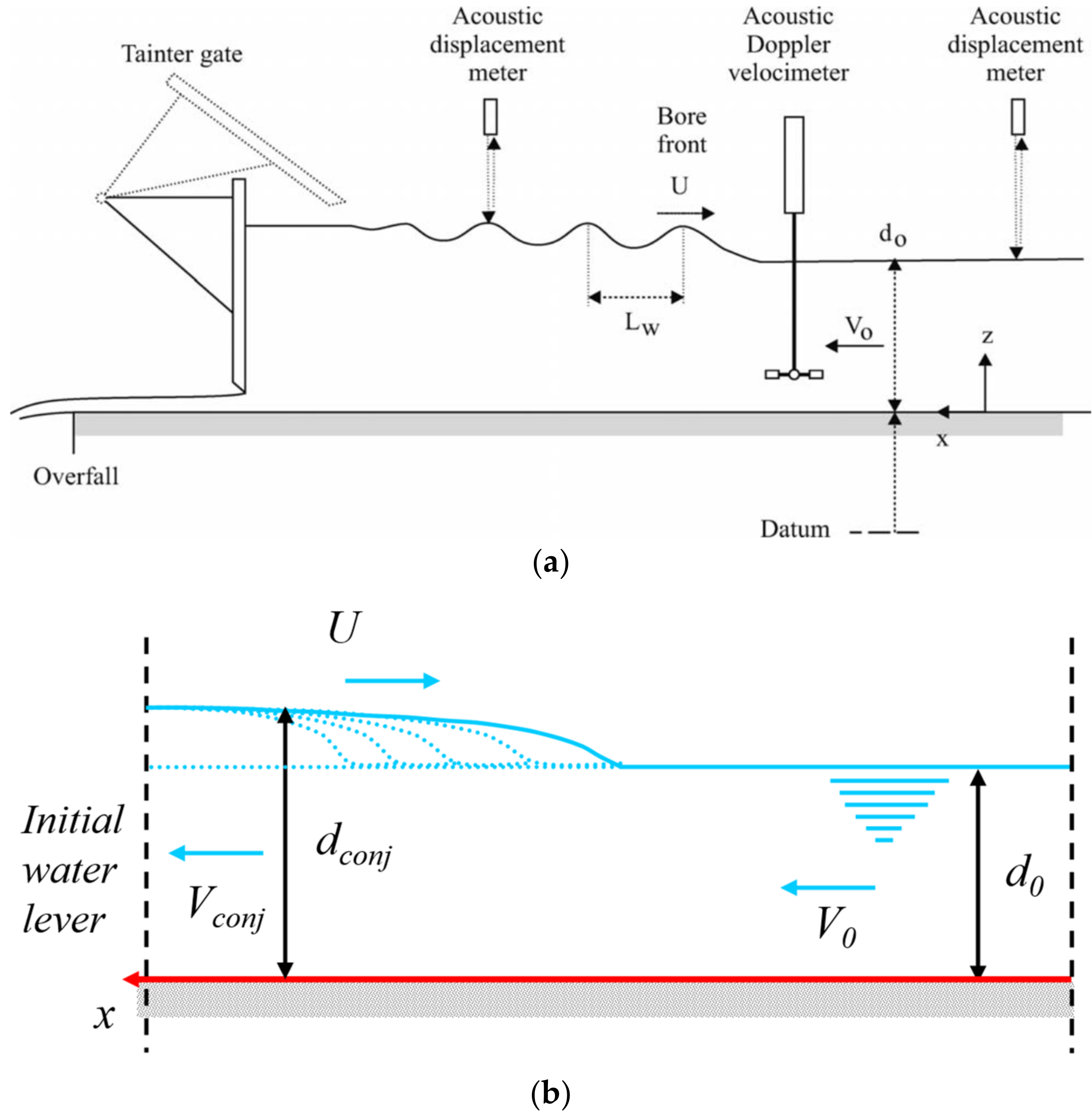
3.1. Channel Setup and Instrumentation
3.2. Generation of the Surge
4. Kolmogorov Complexity and Spectrum: Past Applications and Calculation
4.1. Complexity Measures
4.2. Kolmogorov Complexity
- (1)
- the time series are encoded by creating a sequence S of the characters 0 and 1 written as s(i) = 1, 2, …, N according to the rule s(i) = 0 if xi < xt or s(i) = 1 if xi > xt, where xt a threshold value. The threshold is often selected as the mean value of the time series, while other encoding schemes are also available [28];
- (2)
- the complexity counter c(N), which is the minimum number of distinct patterns contained in a sequence of characters, is computed. The complexity counter c(N), is a function of the sequence length, N, bounded by b(N) = N/log2N, as it approaches infinity, i.e., c(N) = O (b(N));
- (3)
- the normalized information measure Ck (N), which is , is calculated. For a nonlinear time series, Ck (N) ranges from 0 to 1, although it can be larger than 1 for random finite-size sequences.
4.3. Kolmogorov Complexity Spectrum
5. Results
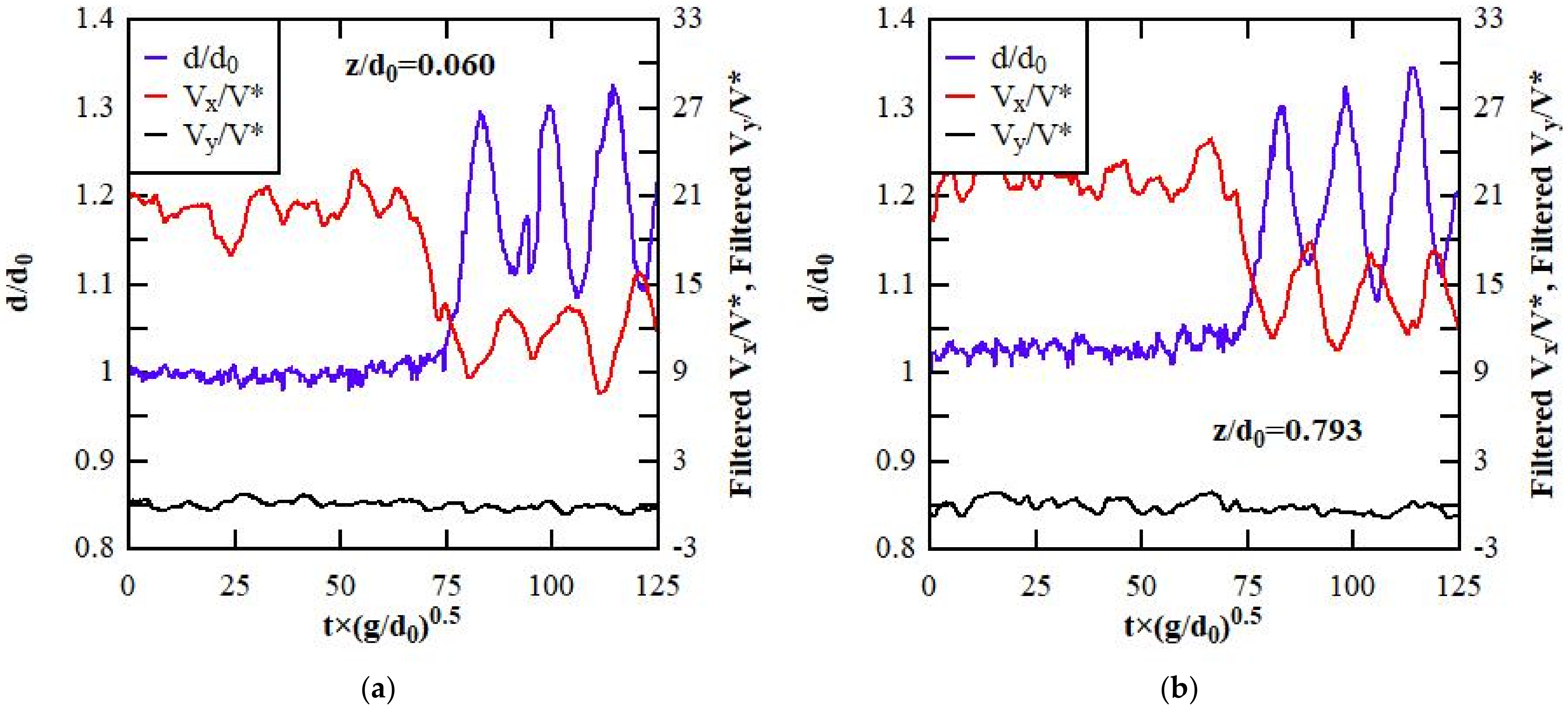
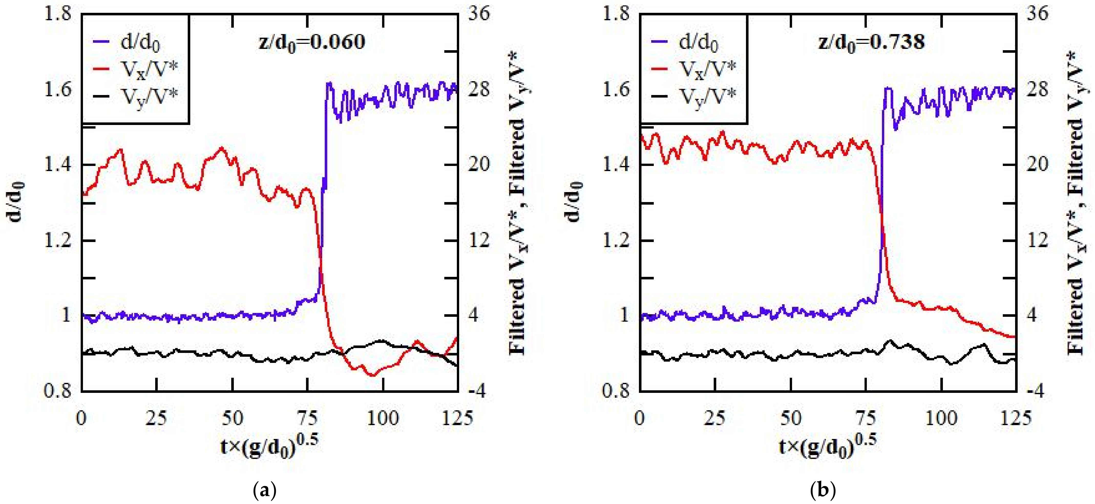
5.1. Time-Variable Depth and Velocity Field
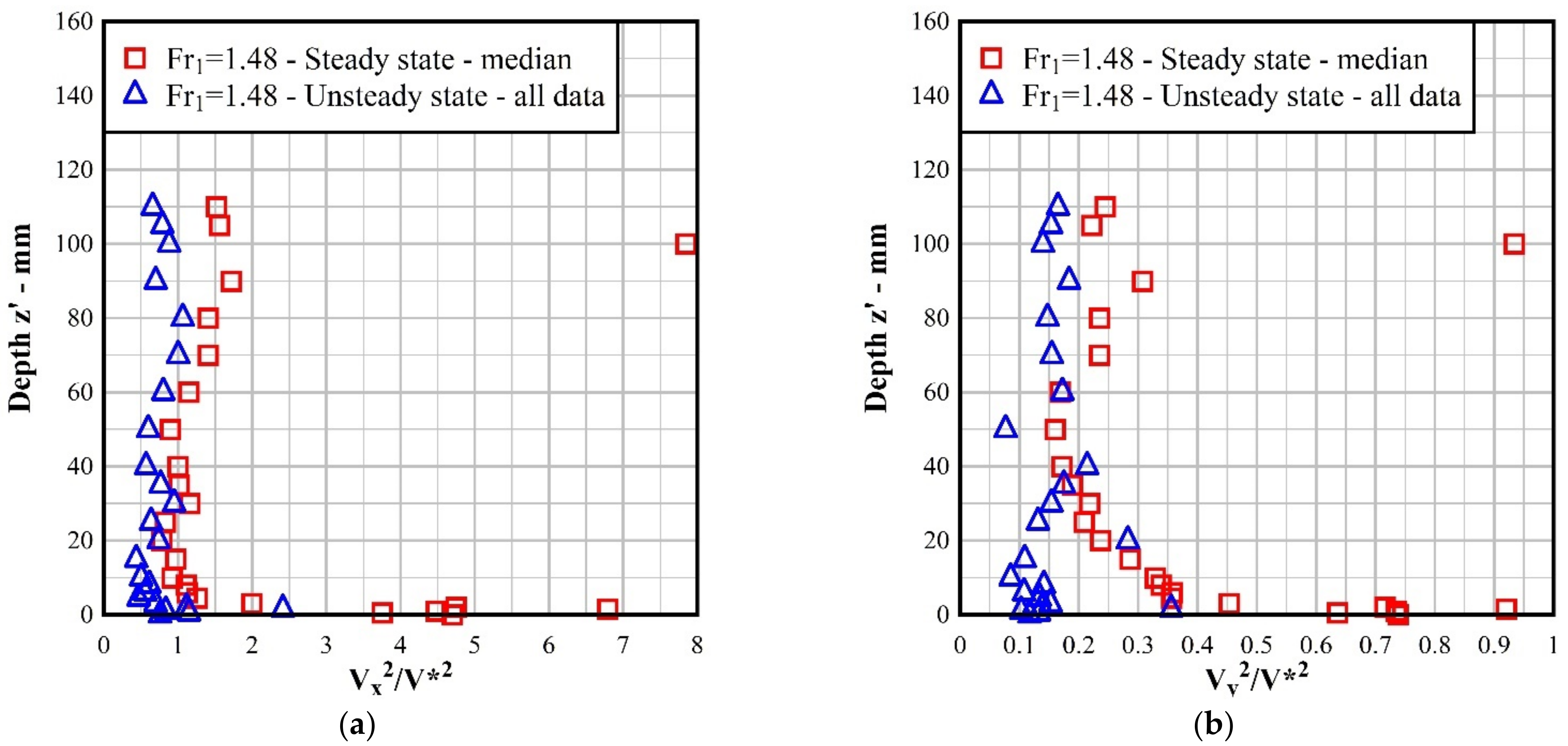
5.2. Reynolds Stresses
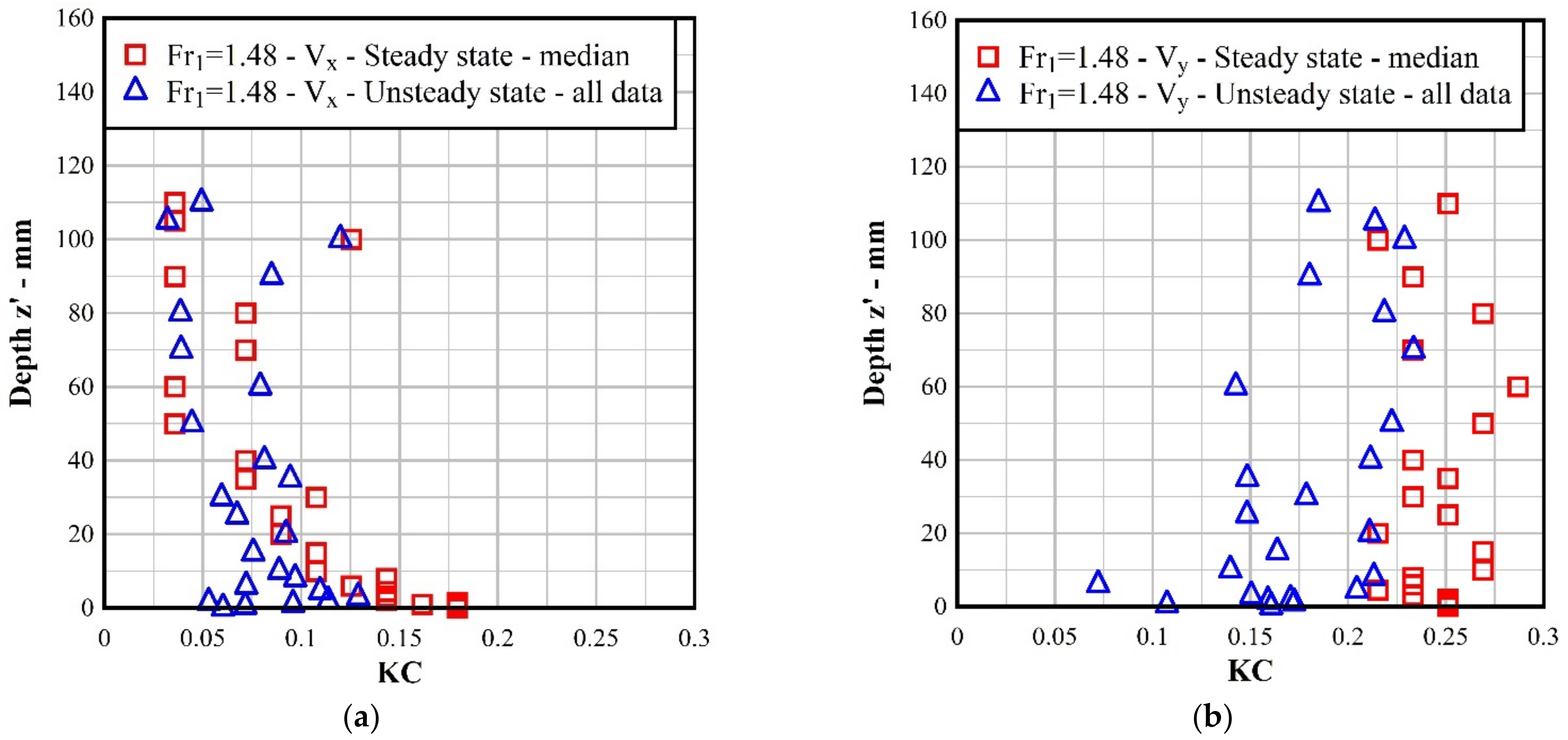
5.3. Kolmogorov Complexity
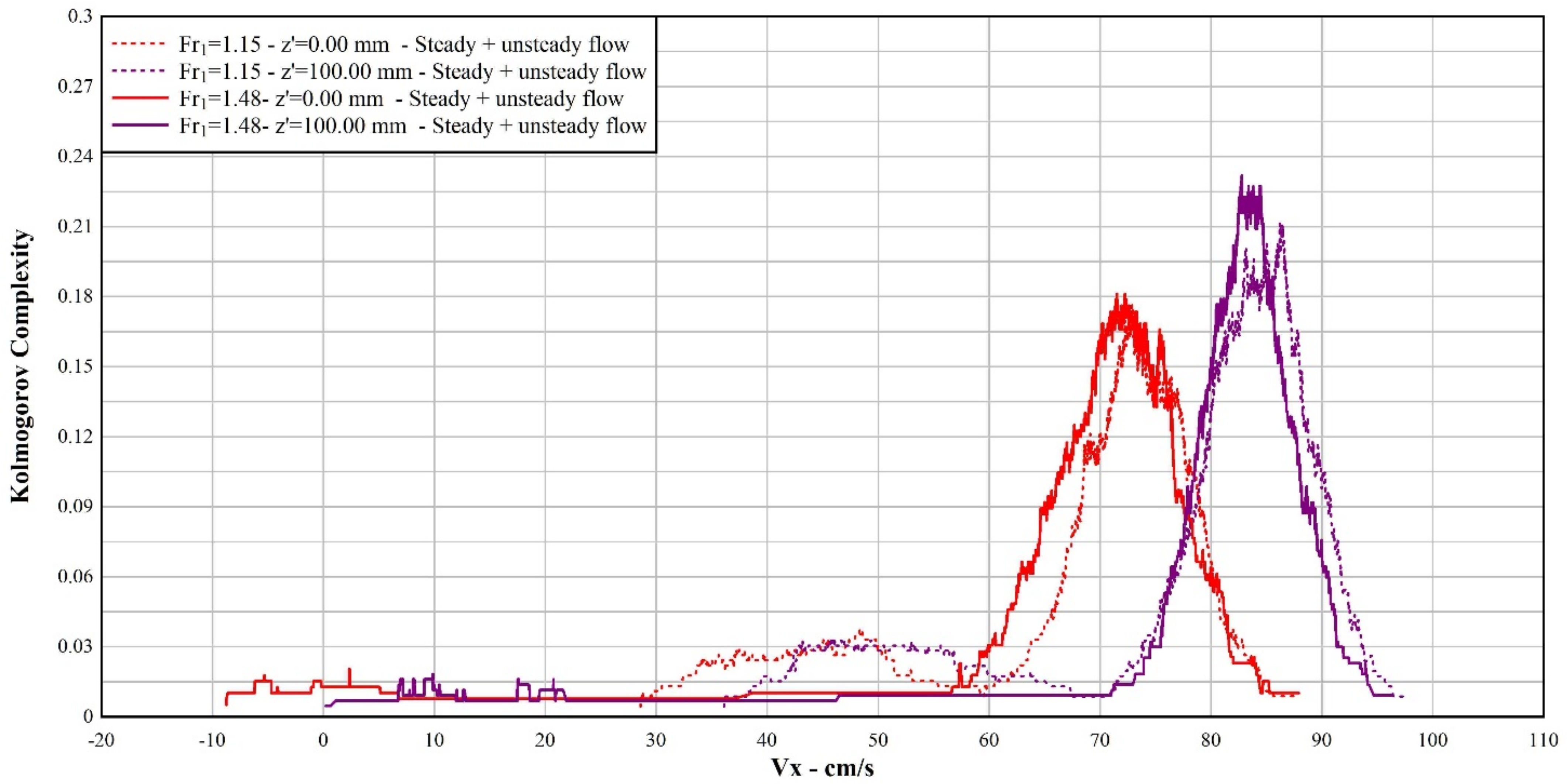
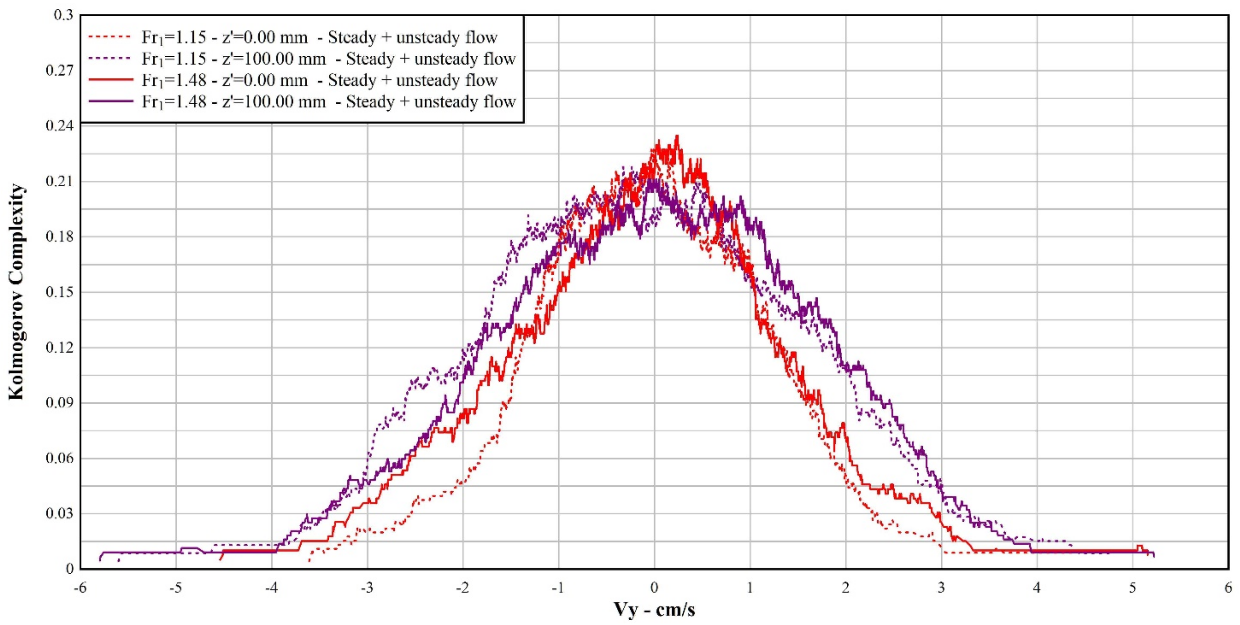
5.4. Kolmogorov Complexity Spectrum
6. Discussion
7. Conclusions
Author Contributions
Funding
Acknowledgments
Conflicts of Interest
References
- Henderson, F.M. Open Channel Flow; MacMillan Company: New York, NY, USA, 1966. [Google Scholar]
- Chow, V.T. Open Channels Hydraulics; Blackburn Press: Caldwell, NJ, USA, 1959; p. 698. [Google Scholar]
- Chanson, H. Environmental fluid dynamics of tidal bores: Theoretical considerations and field observations. In Fluid Mechanics of Environmental Interfaces, 2nd ed.; Gualtieri, C., Mihailović, D.T., Eds.; CRC Press: Boca Raton, FL, USA, 2012; pp. 295–321. [Google Scholar]
- De Saint-Venant, A.J.C.B. Théorie et Equations Générales du Mouvement non Permanent des eaux Courantes; Comptes Rendus des séances de l’Académie des Sciences: Paris, France, 1871; Volume 73, pp. 147–154. (In French) [Google Scholar]
- Boussinesq, J.V. Essai sur la Théorie des eaux Courantes; Essay on the Theory of Water Flow; Mémoires Presents par Divers Savants à l’Académie des Sciences: Paris, France, 1877; Volume 23. (In French) [Google Scholar]
- Favre, H. Etude Théorique et Expérimentale des Ondes de Translation dans les Canaux Découverts; Theoretical and Experimental Study of Travelling Surges in Open Channels; Dunod: Paris, France, 1935. (In French) [Google Scholar]
- Lemoine, R. Sur les Ondes Positives de Translation dans les Canaux et sur le Ressaut Ondulé de Faible Amplitude (On the Positive Surges in Channels and on the Undular Jumps of Low Wave Height). Houille Blanche 1948, 2, 183–185. (In French) [Google Scholar]
- Serre, F. Contribution à L’etude des Ecoulements Permanents et Variables dans les Canaux. Contribution to the Study of Permanent and Non-Permanent Flows in Channels. Houille Blanche 1953, 6, 830–872. (In French) [Google Scholar] [CrossRef] [Green Version]
- Benjamin, T.B.; Lighthill, M.J. On Cnoidal Waves and Bores. Proc. R. Soc. Lond. Series A Math. Phys. Sci. 1954, 224, 448–460. [Google Scholar]
- Peregrine, D.H. Calculations of the development of an undular bore. J. Fluid Mech. 1966, 25, 321–330. [Google Scholar] [CrossRef]
- Sobey, R.J.; Dingemans, M.W. Rapidly varied flow analysis of undular bore. J. Waterw. Port Coastal Ocean Eng. ASCE 1992, 118, 417–436. [Google Scholar] [CrossRef]
- Benet, F.; Cunge, J.A. Analysis of experiments on secondary undulations caused by surge waves in trapezoidal channels. J. Hydraul. Res. IAHR 1971, 9, 11–33. [Google Scholar] [CrossRef]
- Soares Frazão, S.; Zech, Y. Undular bores and secondary waves—Experiments and hybrid finite-volume modelling. J. Hydraul. Res. IAHR 2002, 40, 33–43. [Google Scholar] [CrossRef]
- Treske, A. Undular bores (Favre-waves) in open channels—Experimental studies. J. Hydraul. Res. 1994, 32, 355–370; discussion 33, 274–278. [Google Scholar] [CrossRef]
- Hornung, H.G.; Willert, C.; Turner, S. The flow field downstream of a hydraulic jump. J. Fluid Mech. 1995, 287, 299–316. [Google Scholar] [CrossRef] [Green Version]
- Gualtieri, C.; Chanson, H. Experimental study of hydrodynamics in a positive surge. Part 1: Basic flow patterns and wave attenuation. Environ. Fluid Mech. 2012, 12, 145–159. [Google Scholar] [CrossRef]
- Gualtieri, C.; Chanson, H. Experimental study of hydrodynamics in a positive surge. Part 2: Comparison with literature theories and unsteady flow field analysis. Environ. Fluid Mech. 2011, 11, 641–651. [Google Scholar] [CrossRef]
- Reungoat, D.; Chanson, H.; Caplain, B. Sediment processes and flow reversal in the undular Tidal Bore of the Garonne River (France). Environ. Fluid Mech. 2014, 14, 591–616. [Google Scholar] [CrossRef] [Green Version]
- Leng, X.; Chanson, H.; Reungoat, D. Turbulence and turbulent flux events in tidal bores: Case study of the undular tidal bore of the Garonne River. Environ. Fluid Mech. 2018, 18, 807–828. [Google Scholar] [CrossRef] [Green Version]
- Lubin, P.; Chanson, H.; Glockner, S. Large Eddy Simulation of Turbulence Generated by a Weak Breaking Tidal Bore. Environ. Fluid Mech. 2010, 10, 587–602. [Google Scholar] [CrossRef] [Green Version]
- Nikeghbali, P.; Omidvar, P. Application of the SPH Method to Breaking and Undular Tidal Bores on a Movable Bed. J. Waterw. Port Coastal Ocean Eng. ASCE 2017, 144, 04017040. [Google Scholar] [CrossRef]
- Leng, X.; Simon, B.; Khezri, N.; Lubin, P.; Chanson, H. CFD modeling of tidal bores: Development and validation challenges. Coast. Eng. J. 2018, 60, 423–436. [Google Scholar] [CrossRef]
- Tennekes, H.; Lumley, J.L. A First Course in Turbulence; MIT Press: Cambridge, MA, USA, 1972. [Google Scholar]
- Mihailović, D.T.; Bessafi, M.; Marković, S.; Arsenić, I.; Malinović-Milićević, S.; Jeanty, P.; Delsaut, M.; Chabriat, J.-P.; Drešković, N.; Mihailović, A. Analysis of Solar Irradiation Time Series Complexity and Predictability by Combining Kolmogorov Measures and Hamming Distance for La Reunion (France). Entropy 2018, 20, 570. [Google Scholar] [CrossRef] [Green Version]
- Nagaraj, N.; Balasubramanian, K.; Dey, S. A new complexity measure for time series analysis and classification. Eur. Phys. J. Spec. Top. 2013, 222, 847–860. [Google Scholar] [CrossRef]
- Thilakvathi, B.; Bhanu, K.; Malaippan, M. EEG signal complexity analysis for schizophrenia during rest and mental activity. Biomed. Res. 2017, 28, 1–9. [Google Scholar]
- Cushman-Roisin, B.; Gualtieri, C.; Mihailovic, D.T. Environmental fluid mechanics: Current issues and future outlook. In Fluid Mechanics of Environmental Interfaces, 2nd ed.; Gualtieri, C., Mihailović, D.T., Eds.; CRC Press: Boca Raton, FL, USA, 2012; pp. 3–17. [Google Scholar]
- Mihailović, D.T.; Nikolić-Dorić, E.; Drešković, N.; Mimić, G. Complexity analysis of the turbulent environmental fluid flow time series. Phys. A Stat. Mech. Appl. 2014, 395, 96–104. [Google Scholar] [CrossRef] [Green Version]
- Mihailović, D.T.; Mimić, G.; Drešković, N.; Arsenić, I. Kolmogorov complexity-based information measures applied to the analysis of different river flow regimes. Entropy 2015, 17, 2973–2987. [Google Scholar] [CrossRef] [Green Version]
- Mihailović, D.; Mimić, G.; Gualtieri, P.; Arsenić, I.; Gualtieri, C. Randomness Representation of Turbulence in Canopy Flows Using Kolmogorov Complexity Measures. Entropy 2017, 19, 519. [Google Scholar] [CrossRef] [Green Version]
- Sharma, A.; Mihailović, D.T.; Kumar, B. Randomness representation of Turbulence in an alluvial channel affected by downward seepage. Phys. A 2018, 509, 74–85. [Google Scholar] [CrossRef]
- Lade, A.D.; Mihailović, A.; Mihailović, D.T.; Kumar, B. Randomness in flow turbulence around a bridge pier in a sand mined channel. Phys. A Stat. Mech. Appl. 2019, 535, 122426. [Google Scholar] [CrossRef]
- Ichimiya, M.; Nakamura, I. Randomness representation in turbulent flows with Kolmogorov complexity (in mixing layer). J. Fluid Sci. Technol. 2013, 8, 407–422. [Google Scholar] [CrossRef] [Green Version]
- Khrennikov, A. Introduction to foundations of probability and randomness (for students in physics), Lectures given at the Institute of Quantum Optics and Quantum Information, Austrian Academy of Science, Lecture-1: Kolmogorov and von Mises. arXiv 2014, arXiv:1410.5773. [Google Scholar]
- Kolmogorov, A. Three approaches to the quantitative definition of information. Probl. Inf. Transm. 1965, 1, 4. [Google Scholar] [CrossRef]
- Mihailović, D.T.; Balaž, I.; Kapor, D. Time and Methods in Environmental Interfaces Modeling: Personal Insights; Elsevier: Amsterdam, The Netherlands, 2016; p. 426. [Google Scholar]
- Mihailović, D.T.; Mihailović, A.; Gualtieri, C.; Kapor, D. How to assimilate hitherto inaccessible information in environmental sciences ? Modelling for sustainability. In Proceedings of the iEMSs Tenth Biennial Meeting: International Congress on Environmental Modelling and Software (iEMSs 2020), Bruxelles, Belgium, 14–18 September 2020. [Google Scholar]
- Damasio, A. Looking for Spinoza: Joy, Sorrow, and the Feeling Brain; Harcourt: Orlando, FL, USA, 2003. [Google Scholar]
- Osterlund, J.M. Experimental Studies of Zero Pressure-Gradient Turbulent Boundary Layer Flow. Ph.D. Thesis, Department of Mechanics, Royal Institute of Technology, Stockholm, Sweden, 1999. Available online: http://www2.mech.kth.se/~jens/zpg/index.html (accessed on 5 May 2021).
- Lempel, A.; Ziv, J. On the complexity of finite sequences. IEEE Trans. Inform. Theory 1976, 22, 75–81. [Google Scholar] [CrossRef]
- Gualtieri, C.; Pulci Doria, G. Gas-transfer at unsheared free surfaces. In Fluid Mechanics of Environmental Interfaces, 2nd ed.; Gualtieri, C., Mihailović, D.T., Eds.; CRC Press: Boca Raton, FL, USA, 2012; pp. 143–177. [Google Scholar]
- Rodi, W.; Constantinescu, G.; Stoesser, T. Large-Eddy Simulation in Hydraulics; CRC Press: New York, NY, USA, 2013. [Google Scholar]
- Chanson, H.; Toi, Y.H. Physical Modelling of Breaking Tidal Bores: Comparison with Prototype Data. J. Hydraul. Res. IAHR 2015, 53, 264–273. [Google Scholar] [CrossRef] [Green Version]
- Hinze, J.O. Turbulence, 2nd ed.; McGraw-Hill: New York, NY, USA, 1975. [Google Scholar]
- Leng, X.; Chanson, H. Integral Turbulent Scales in Unsteady Rapidly Varied Open Channel Flows. Expe. Therm. Fluid Sci. 2017, 81, 382–395. [Google Scholar] [CrossRef] [Green Version]
- Docherty, N.J.; Chanson, H. Physical modelling of unsteady turbulence in breaking tidal bores. J. Hydraul. Eng. ASCE 2012, 138, 412–419. [Google Scholar] [CrossRef] [Green Version]
- Chanson, H. Statistical Analysis Method for Transient Flows—The Dam-Break Case. Discussion. J. Hydraul. Res. IAHR 2020, 58, 1001–1004. [Google Scholar] [CrossRef]


| Run | Q—m3/s | d0—m | hg—m | Type | U—m/s | dconj—m | Fr1 | Remarks |
|---|---|---|---|---|---|---|---|---|
| 60-6 | 0.060 | 0.1429 | 0.005 | Breaking | 0.918 | 0.237 | 1.484 | ADV measurements |
| 60-7 | 0.060 | 0.1427 | 0.100 | Undular | 0.519 | 0.171 | 1.149 | ADV measurements |
Publisher’s Note: MDPI stays neutral with regard to jurisdictional claims in published maps and institutional affiliations. |
© 2022 by the authors. Licensee MDPI, Basel, Switzerland. This article is an open access article distributed under the terms and conditions of the Creative Commons Attribution (CC BY) license (https://creativecommons.org/licenses/by/4.0/).
Share and Cite
Gualtieri, C.; Mihailović, A.; Mihailović, D. An Application of Kolmogorov Complexity and Its Spectrum to Positive Surges. Fluids 2022, 7, 162. https://doi.org/10.3390/fluids7050162
Gualtieri C, Mihailović A, Mihailović D. An Application of Kolmogorov Complexity and Its Spectrum to Positive Surges. Fluids. 2022; 7(5):162. https://doi.org/10.3390/fluids7050162
Chicago/Turabian StyleGualtieri, Carlo, Anja Mihailović, and Dragutin Mihailović. 2022. "An Application of Kolmogorov Complexity and Its Spectrum to Positive Surges" Fluids 7, no. 5: 162. https://doi.org/10.3390/fluids7050162
APA StyleGualtieri, C., Mihailović, A., & Mihailović, D. (2022). An Application of Kolmogorov Complexity and Its Spectrum to Positive Surges. Fluids, 7(5), 162. https://doi.org/10.3390/fluids7050162