
Optimization of a Micromixer with Automatic Differentiation

 , ,
, ,
Abstract
:1. Introduction
2. Materials and Methods
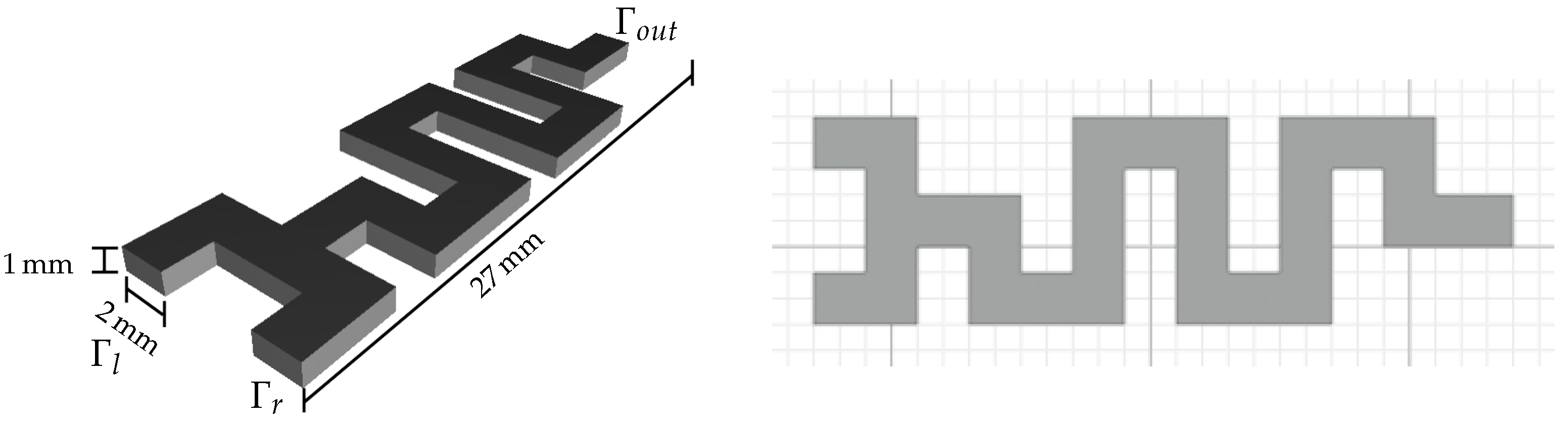
2.1. Experimental Design
2.2. Fluid Flow Model
2.3. Discretization with a Lattice Boltzmann Method
2.4. Optimization Setup
2.5. Automatic Differentiation
2.6. Numerical Optimization
3. Results
3.1. Simulation
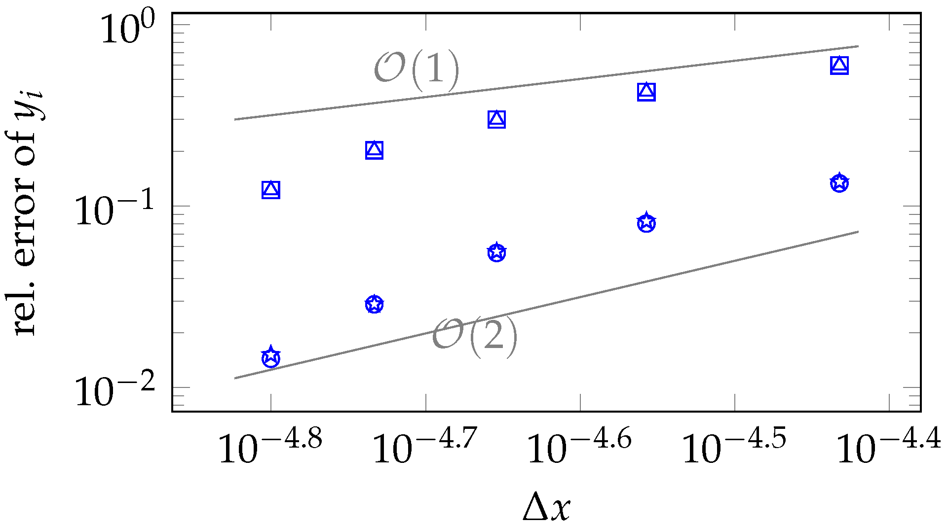
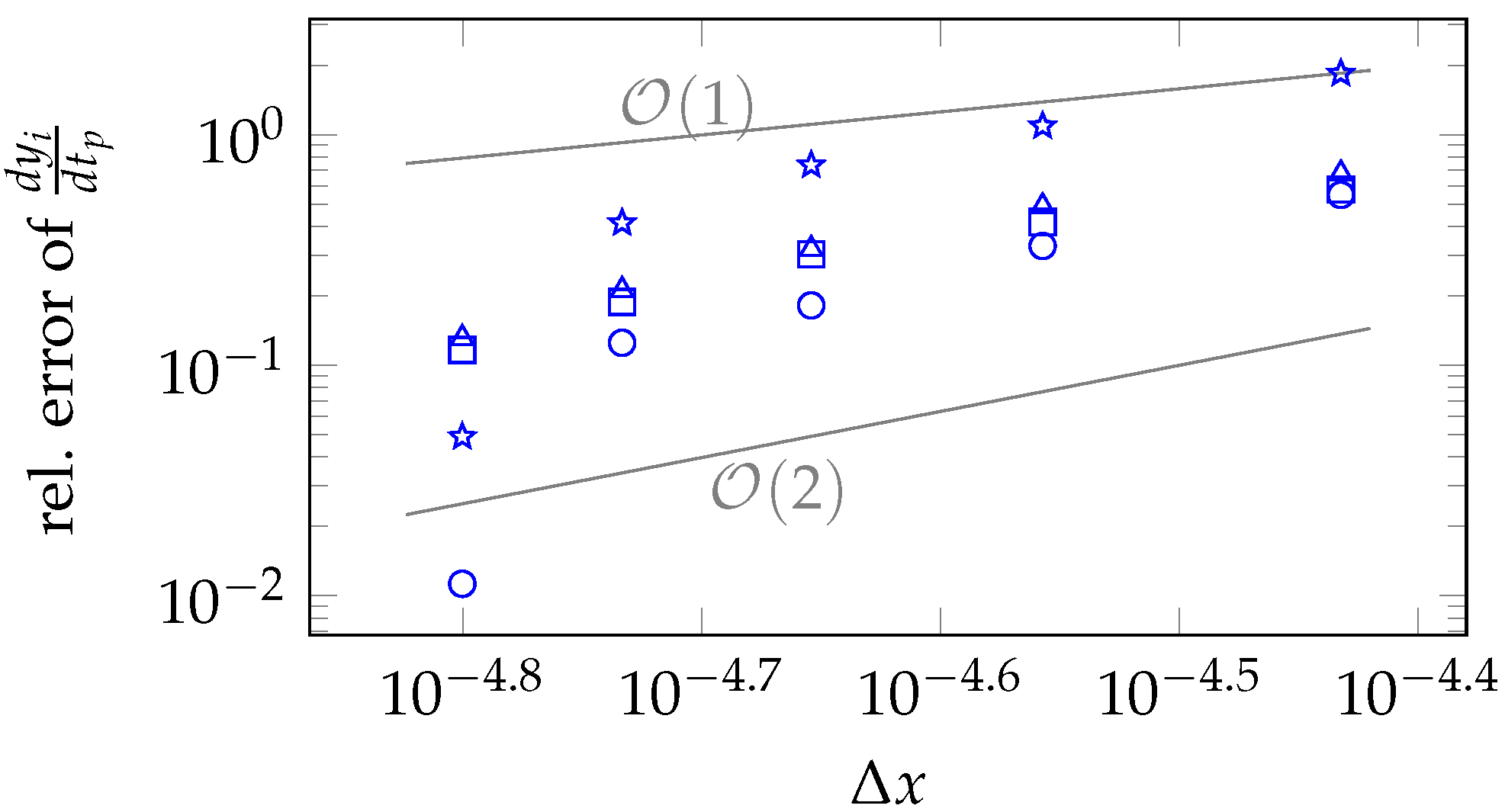
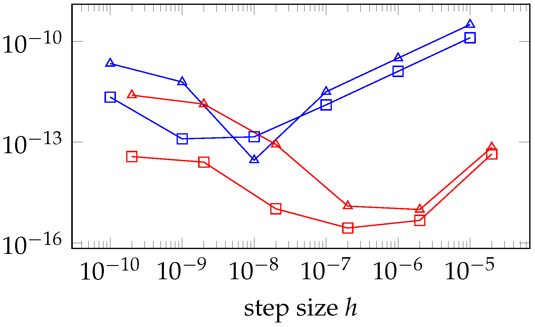
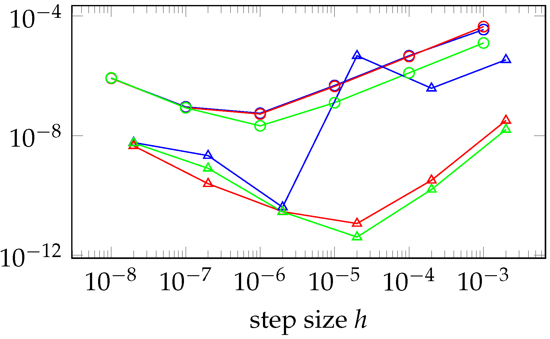
3.2. Simulation of Sensitivities
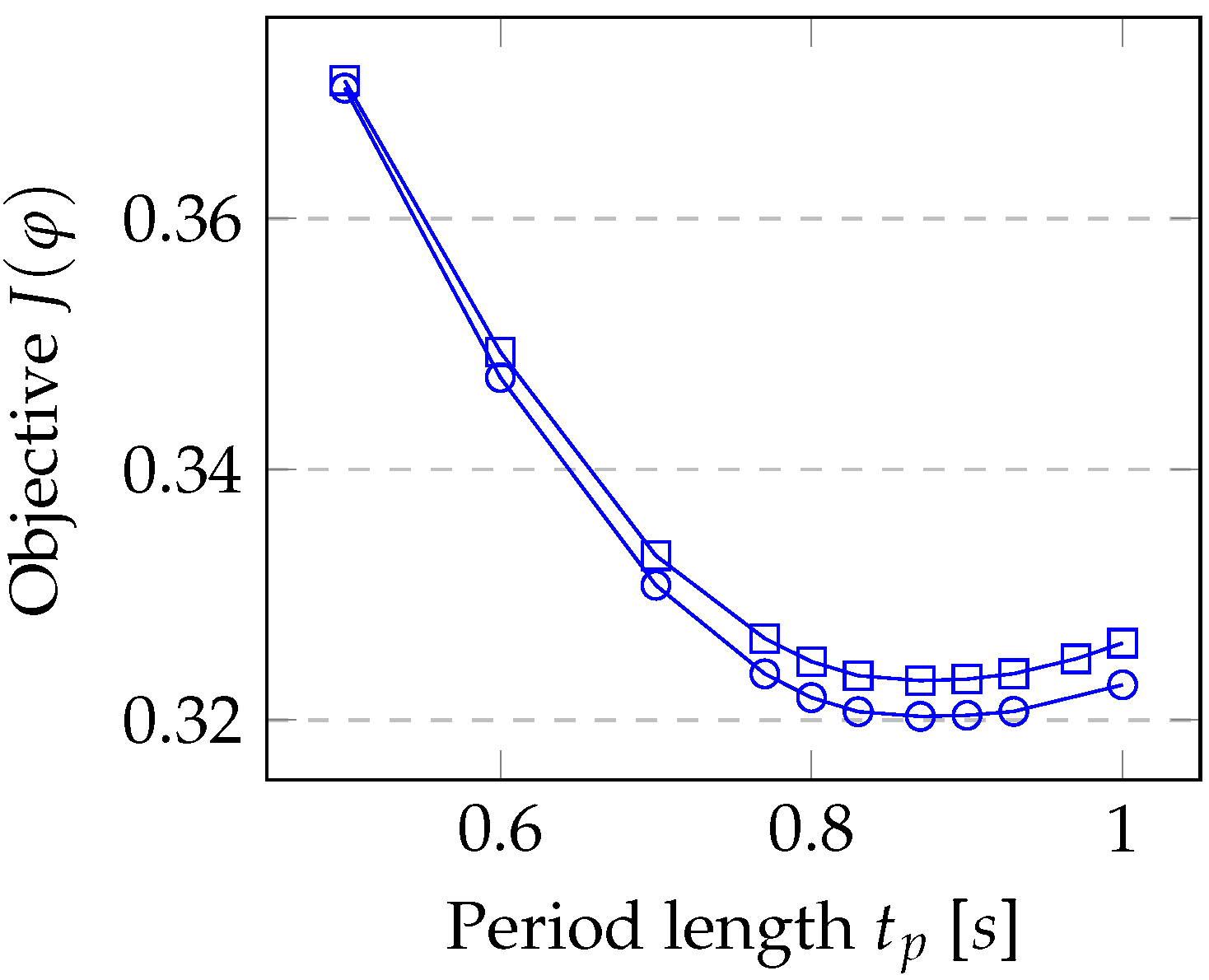
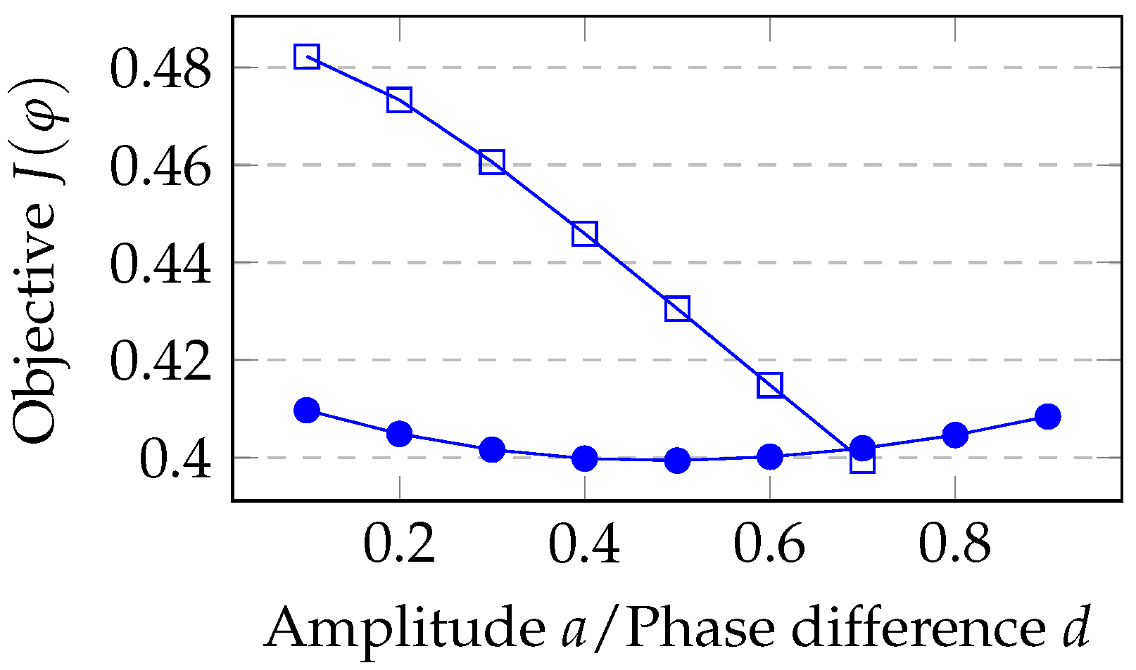
3.3. Optimization
4. Discussion
5. Conclusions
Author Contributions
Funding
Institutional Review Board Statement
Informed Consent Statement
Data Availability Statement
Acknowledgments
Conflicts of Interest
Nomenclature
| AD | Automatic differentiation |
| ADE | Advection–diffusion equation |
| BGK | Bhatnagar–Gross–Krook |
| CDQ | Central difference quotient |
| CFD | Computational fluid dynamics |
| FDQ | Forward difference quotient |
| FEM | Finite element method |
| LBM | Lattice Boltzmann methods |
| NSE | Navier–Stokes equations |
| Constants, parameters and variables: | |
| , | temporal and spatial resolution |
| , , , | boundary of the domain (left inlet, right inlet, outlet, wall) |
| flow channel | |
| smoothing width for | |
| kinematic viscosity | |
| relative mass concentration of adsorptive particles | |
| fluid density | |
| variance of at the outlet over | |
| D | diffusion coefficient |
| average of at the outlet over | |
| segregation intensity at the outlet over | |
| mixing quality at the outlet over | |
| I | temporal simulation interval |
| L | hydraulic channel diameter |
| Péclet number | |
| Reynolds number | |
| T | max. simulation time |
| U | char. fluid velocity |
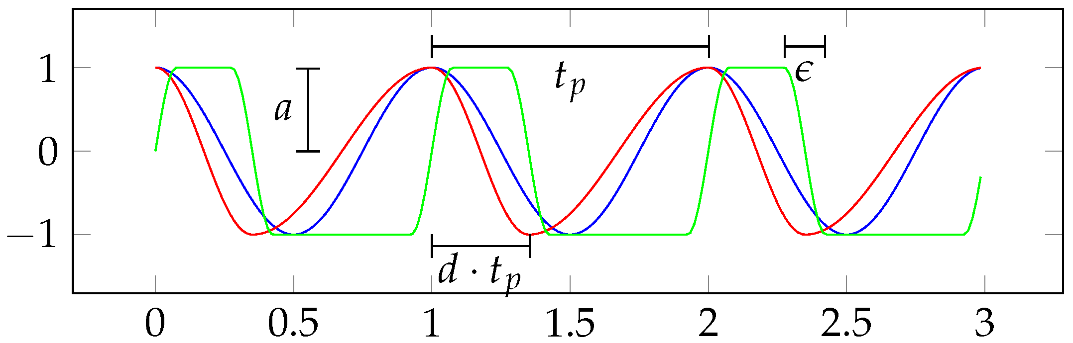
| a | amplitude of inlet phase function |
| d | phase difference in inlet phase function |
| h | step width for FDQ/CDQ |
| p | kinematic pressure |
| time-dependent pressure at the right inlet | |
| periodic inlet phase function: composite cosine | |
| periodic inlet phase function: smoothed square wave | |
| start-up function for velocity at the outlet | |
| t | temporal coordinate |
| , | start-up time for outflow and pressure pulse, resp. |
| period length of inlet phase function | |
| , , | fluid velocity (3D vector, tangential to the boundary, normal to the boundary) |
| velocity profile at the outlet (normal component) | |
| spatial coordinates | |
| -norm of at the left inlet at | |
| -norm of at the outlet at | |
References
- Hardt, S.; Schönfeld, F. Microfluidic Technologies for Miniaturized Analysis Systems; Springer Science + Business Media, LLC: New York, NY, USA, 2007; Volume 392. [Google Scholar] [CrossRef]
- Hessel, V.; Löwe, H.; Schönfeld, F. Micromixers—A review on passive and active mixing principles. Chem. Eng. Sci. 2005, 60, 2479–2501. [Google Scholar] [CrossRef]
- Raza, W.; Hossain, S.; Kim, K.Y. A Review of Passive Micromixers with a Comparative Analysis. Micromachines 2020, 11, 455. [Google Scholar] [CrossRef] [PubMed]
- Glasgow, I.; Aubry, N. Enhancement of microfluidic mixing using time pulsing. Lab Chip 2003, 3, 114–120. [Google Scholar] [CrossRef] [PubMed]
- Danckwerts, P.V. The Definition and Measurement of Some Characteristics of Mixtures. Appl. Sci. Res. Sect. A 1952, 3, 279–296. [Google Scholar] [CrossRef]
- Khaydarov, V.; Borovinskaya, E.S.; Reschetilowski, W. Numerical and Experimental Investigations of a Micromixer with Chicane Mixing Geometry. Appl. Sci. 2018, 8, 2458. [Google Scholar] [CrossRef] [Green Version]
- Ahmad Termizi, S.N.A.; Khor, C.Y.; Nawi, M.A.H.; Ahmad, N.; Ishak, M.; Rosli, M.; Jamalludin, M. Computational Fluid Dynamics (CFD) Simulation on Mixing in T-Shaped Micromixer. IOP Conf. Ser. Mater. Sci. Eng. 2020, 932, 012006. [Google Scholar] [CrossRef]
- Termizi, S.N.A.A.; Ishak, M.I.; Khor, C.Y.; Nawi, M.A.M.; Pouzay, M.F.B.M. Computational fluid dynamics (CFD) simulation on mixing in Y-shaped micromixer. AIP Conf. Proc. 2020, 2291, 020048. [Google Scholar] [CrossRef]
- Rudyak, V.; Minakov, A. Modeling and Optimization of Y-Type Micromixers. Micromachines 2014, 5, 886–912. [Google Scholar] [CrossRef]
- Maier, M.L.; Milles, S.; Schuhmann, S.; Guthausen, G.; Nirschl, H.; Krause, M.J. Fluid flow simulations verified by measurements to investigate adsorption processes in a static mixer. Comput. Math. Appl. 2018, 76, 2744–2757. [Google Scholar] [CrossRef]
- Santana, H.S.; Silva, J.L.; Taranto, O.P. Optimization of micromixer with triangular baffles for chemical process in millidevices. Sens. Actuators B Chem. 2019, 281, 191–203. [Google Scholar] [CrossRef]
- Hossain, S.; Ansari, M.; Husain, A.; Kim, K.Y. Analysis and optimization of a micromixer with a modified Tesla structure. Chem. Eng. J. 2010, 158, 305–314. [Google Scholar] [CrossRef]
- Bockelmann, H.; Heuveline, V.; Barz, D.P.J. Optimization of an electrokinetic mixer for microfluidic applications. Biomicrofluidics 2012, 6, 024123. [Google Scholar] [CrossRef] [PubMed] [Green Version]
- Bockelmann, H. High Performance Computing Based Methods for Simulation and Optimisation of Flow Problems. Ph.D. Thesis, Karlsruher Institut für Technologie, Karlsruhe, Germany, 2010. [Google Scholar] [CrossRef]
- Gunzburger, M.D. Perspectives in Flow Control and Optimization; Society for Industrial and Applied Mathematics: Philadelphia, PA, USA, 2002. [Google Scholar] [CrossRef]
- Krause, M.J. Fluid Flow Simulation and Optimisation with Lattice Boltzmann Methods on High Performance Computers—Application to the Human Respiratory System. Ph.D. Thesis, Karlsruher Institut für Technologie, Karlsruhe, Germany, 2010. [Google Scholar]
- Krause, M.J.; Heuveline, V. Parallel Fluid Flow Control and Optimisation with Lattice Boltzmann Methods and Automatic Differentiation. Comput. Fluids 2013, 80, 28–36. [Google Scholar] [CrossRef]
- Nørgaard, S.; Sagebaum, M.; Gauger, N.; Lazarov, B. Applications of automatic differentiation in topology optimization. Struct. Multidiscip. Optim. 2017, 56. [Google Scholar] [CrossRef]
- Zarth, A.; Klemens, F.; Thäter, G.; Krause, M.J. Towards shape optimisation of fluid flows using lattice Boltzmann methods and automatic differentiation. Comput. Math. Appl. 2021, 90, 46–54. [Google Scholar] [CrossRef]
- Trunk, R.; Henn, T.; Dörfler, W.; Nirschl, H.; Krause, M.J. Inertial dilute particulate fluid flow simulations with an Euler–Euler lattice Boltzmann method. J. Comput. Sci. 2016, 17, 438–445. [Google Scholar] [CrossRef]
- Krüger, T.; Kusumaatmaja, H.; Kuzmin, A.; Shardt, O.; Silva, G.; Viggen, E.M. The Lattice Boltzmann Method—Principles and Practice; Springer: Cham, Switzerland, 2016. [Google Scholar] [CrossRef]
- Bhatnagar, P.L.; Gross, E.P.; Krook, M. A Model for Collision Processes in Gases. I. Small Amplitude Processes in Charged and Neutral One-Component Systems. Phys. Rev. 1954, 94, 511–525. [Google Scholar] [CrossRef]
- Gruszczyński, G.; Dzikowski, M.; Wołłk, Ł.Ł. On recovering the second-order convergence of the lattice Boltzmann method with reaction-type source terms. arXiv 2021, arXiv:2107.03962. [Google Scholar]
- Schornbaum, F.; Rüde, U. Extreme-Scale Block-Structured Adaptive Mesh Refinement. SIAM J. Sci. Comput. 2018, 40, C358–C387. [Google Scholar] [CrossRef] [Green Version]
- Courant, R.; Isaacson, E.; Rees, M. On the solution of nonlinear hyperbolic differential equations by finite differences. Commun. Pure Appl. Math. 1952, 5, 243–255. [Google Scholar] [CrossRef]
- Latt, J.; Chopard, B.; Malaspinas, O.; Deville, M.; Michler, A. Straight velocity boundaries in the lattice Boltzmann method. Phys. Rev. E 2008, 77, 056703. [Google Scholar] [CrossRef] [PubMed]
- Latt, J. Hydrodynamic Limit of Lattice Boltzmann Equations. Ph.D. Thesis, Université de Genève, Genève, Switzerland, 2007. [Google Scholar]
- Skordos, P.A. Initial and boundary conditions for the lattice Boltzmann method. Phys. Rev. E 1993, 48, 4823–4842. [Google Scholar] [CrossRef] [PubMed] [Green Version]
- Mangold, J. Optimierung Eines Statischen Mischers Mittels Kontrolle der Eingangsströmung. Bachelor’s Thesis, Karlsruhe Institute of Technology, Karlsruhe, Germany, 2019. [Google Scholar]
- Bothe, D.; Stemich, C.; Warnecke, H.J. Fluid mixing in a T-shaped micro-mixer. Chem. Eng. Sci. 2006, 61, 2950–2958. [Google Scholar] [CrossRef]
- Sauer, T. Numerical Analysis, 2nd ed.; Featured Titles for Numerical Analysis; Pearson: London, UK, 2011. [Google Scholar]
- Griewank, A.; Walther, A. Evaluating Derivatives, 2nd ed.; Society for Industrial and Applied Mathematics (SIAM): Philadelphia, PA, USA, 2008. [Google Scholar] [CrossRef]
- Krause, M.J.; Avis, S.; Kusumaatmaja, H.; Dapelo, D.; Gaedtke, M.; Hafen, N.; Haußmann, M.; Jeppener-Haltenhoff, J.; Kronberg, L.; Kummerländer, A.; et al. OpenLB Release 1.4: Open Source Lattice Boltzmann Code; Zenodo: Genève, Switzerland, 2020. [Google Scholar] [CrossRef]
- Krause, M.J.; Kummerländer, A.; Avis, S.J.; Kusumaatmaja, H.; Dapelo, D.; Klemens, F.; Gaedtke, M.; Hafen, N.; Mink, A.; Trunk, R.; et al. OpenLB—Open source lattice Boltzmann code. Comput. Math. Appl. 2021, 81, 258–288. [Google Scholar] [CrossRef]
- Geiger, C.; Kanzow, C. Numerische Verfahren zur Lösung Unrestringierter Optimierungsaufgaben; Springer: Berlin, Germany, 1999. [Google Scholar]
- Byrd, R.H.; Lu, P.; Nocedal, J.; Zhu, C. A Limited Memory Algorithm for Bound Constrained Optimization. SIAM J. Sci. Comput. 1995, 16, 1190–1208. [Google Scholar] [CrossRef]


| Period Length in s | over | over | Relative Difference |
|---|---|---|---|
| Parameter | Value |
|---|---|
| Char. velocity U | |
| Hydraulic channel diameter L | |
| Reynolds number | |
| Mass diffusivity D | |
| Fluid density | |
| Viscosity | |
| Péclet number | 44,156 |
Publisher’s Note: MDPI stays neutral with regard to jurisdictional claims in published maps and institutional affiliations. |
© 2022 by the authors. Licensee MDPI, Basel, Switzerland. This article is an open access article distributed under the terms and conditions of the Creative Commons Attribution (CC BY) license (https://creativecommons.org/licenses/by/4.0/).
Share and Cite
Jeßberger, J.; Marquardt, J.E.; Heim, L.; Mangold, J.; Bukreev, F.; Krause, M.J. Optimization of a Micromixer with Automatic Differentiation. Fluids 2022, 7, 144. https://doi.org/10.3390/fluids7050144
Jeßberger J, Marquardt JE, Heim L, Mangold J, Bukreev F, Krause MJ. Optimization of a Micromixer with Automatic Differentiation. Fluids. 2022; 7(5):144. https://doi.org/10.3390/fluids7050144
Chicago/Turabian StyleJeßberger, Julius, Jan E. Marquardt, Luca Heim, Jakob Mangold, Fedor Bukreev, and Mathias J. Krause. 2022. "Optimization of a Micromixer with Automatic Differentiation" Fluids 7, no. 5: 144. https://doi.org/10.3390/fluids7050144
APA StyleJeßberger, J., Marquardt, J. E., Heim, L., Mangold, J., Bukreev, F., & Krause, M. J. (2022). Optimization of a Micromixer with Automatic Differentiation. Fluids, 7(5), 144. https://doi.org/10.3390/fluids7050144