1. Introduction
The Japan Sea is a marginal sea with shallow straits of water exchange with the Pacific Ocean. It is a deep basin (more than 3500 m) with intense vertical mixing due to winter convection, with a system of boundary currents, a subarctic frontal zone and quasi-stationary and drifting mesoscale eddies. The Japan Sea is a miniature model of the ocean and an indicator of climate change over the adjacent part of the continent. The maximum distribution of dissolved oxygen content at a depth of 1 km for the whole Pacific Ocean has been observed in this sea [
1]. That indicates the intense processes of vertical mixing and renewal of deep waters taking place here. Differences in the estimates of the rate of renewal of the deep water in the sea indicate a considerable interannual variability of this renewal [
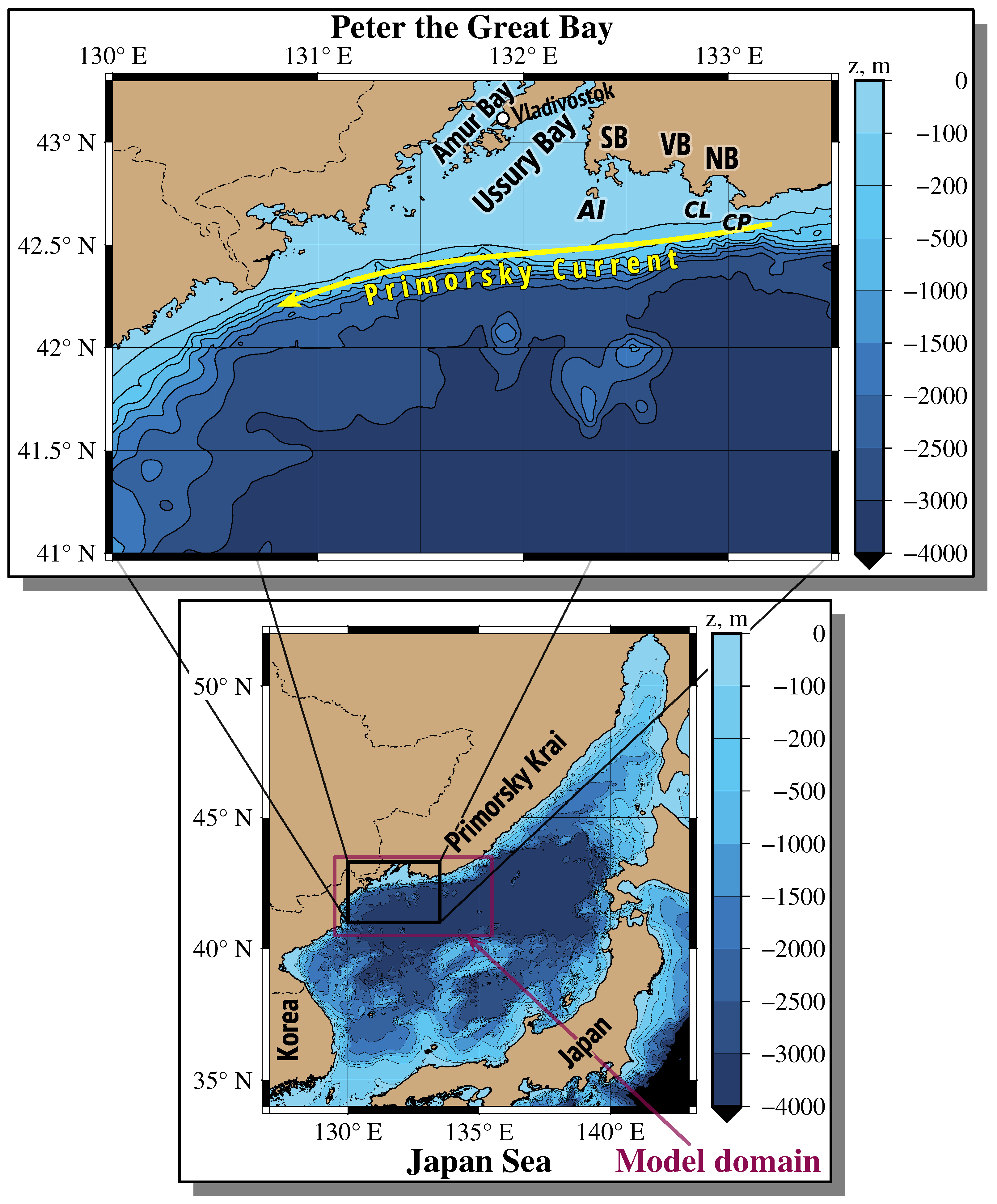
1]. The main process of bottom water ventilation is winter slope convection in the area of Peter the Great Bay (PGB), a vast bay south of Vladivostok city (
Figure 1).
The circulation in PGB is characterized by a high seasonal and synoptic variability (see the monthly mean surface currents in
Figures S1 and S2 in Supplementary Materials). The Primorsky Current flows along the continental slope with the maximum current velocities in fall–winter (40 cm/s) and with the minimal ones in spring–summer (15–20 cm/s). From March to July, cyclonic circulation prevails in the open part of PGB. From the end of summer and in the fall–winter period, anticyclonic circulation prevails in the open part of PGB. The anticyclonic circulation prevails in the central and northern parts of the Ussury Bay, whereas the cyclonic circulation prevails in the southern part of this bay. A complex circulation is observed in the Amur Bay, including a lot of eddies, mainly, with anticyclonic polarity. Numerous eddies of various size and polarity are regularly observed in the open part of PGB. Cyclonic eddies usually form in the area of Cape Likhachev, whereas anticyclonic eddies form in the area of Cape Povorotny and Nakhodka Bay (
Figure 1). In wintertime, the northwesterly and northly winds maintain coastal polynyas in PGB with continuous ice formation and brine rejection that give rise to the formation of high-density water and its deep convection.
The descent of dense water down a continental slope to greater than 1000 m depth is known as “deep slope convection” (DSC). It is an important process in the formation of intermediate and bottom waters that has been observed at a few select locations in some semi-enclosed seas (see e.g., [
2,
3]). The resulting formation of these water masses and deep ventilation are of importance to physics and dynamics of these local seas. It has long been thought that the dense shelf water (DSW) formation occurs in wintertime south of Vladivostok (see, e.g., [
4,
5]), but definitive evidence has not been found until the winter surveys in the 1990s of the last century [
6], in 2000–2001 [
7,
8,
9,
10], and later [
11]. The descent of DSW down the continental slope led to the formation of new bottom water at the foot of the slope. New bottom water was observed in 28 February–15 March 2000 and in 24 February–3 March 2001 between 2000 and 3000 m along the meridional section
(
–
) [
10]. This water was also observed in 14–24 April 2001 at the depth of 3000 m along the meridional section
(
–
) [
8,
9].
The steep continental slope of PGB with deep canyons and dry cold winters in the area provide suitable conditions for the implementation of DSC. According to the results of measurements in different winters, it has been established that every year from the end of January to the middle of April a high-density water mass episodically approaches the shelf edge. The duration of such episodes ranges from several hours to several days. Penetration of anomalously cold water down the middle of the slope (at depths of 1000–1200 m) was recorded in the second half of February practically every winter in the period from 2010 to 2017. Clear signs of the penetration of DSW in the lowest part of the slope and at its foot, i.e., deeper than 2000 m, were observed in PGB in a few winters only: in 1997 [
6], 2001 [
10], and 2018 [
11]. The DSC events do not occur every winter despite intense surface cooling. It is a rare phenomenon with interannual variability [
12].
Observations of DSC are rare and sparse, since it is hard to be at the right place and at the right time when this phenomenon occurs. Consequently, observational data are not enough to understand and study the initiation, evolution, and termination of DSC events. This requires the use of realistic numerical models with high resolution in order to detect episodes with formation of DSW on a shelf, advection to the slope edge, and descent down the slope. As to the simulation of the stream path of the descending plume, [
12] conducted a series of numerical experiments using a simple streamtube model [
13], which allows a quantitative estimate of the depth of the DSW descent.
The main objective of the present paper is to use the ROMS (Regional Ocean Modeling System) with a 600 m resolution to simulate with the help of Lagrangian methods: (i) formation of DSW on a shallow shelf; (ii) its advection to the slope edge; (iii) impact of coastal eddies in the eastern part of PGB on the cross-shelf transport of DSW; and (iv) its subsequent descent down the slope. We also compare the simulation results with shipboard observations of DSC in PGB in the extremely cold winter of 2001 and with some records of DSW by a profiler “Aqualog” installed at the shelf break in the regular winter of 2010.
2. Numerical Model
The circulation in PGB was modeled by the Regional Ocean Modeling System (ROMS,
www.myroms.org, access date: 6 March 2021), which is a free-surface, nonlinear, primitive equation model featuring terrain-following coordinates in the vertical and advanced numerics [
14]. The model domain (
Figure 1), vertical and horizontal resolution, numerical schemes for vertical turbulence forcing, and bulk flux formulation were the same as in [
15]. The surface wind speed was obtained from the Daily ASCAT global wind field with the
uniform horizontal resolution [
16]. Air pressure, incoming shortwave radiation, relative humidity, air temperature, precipitation, and cloud cover were obtained from the NCEP-DOE AMIP-II Reanalysis. Daily fields of sea surface temperature, obtained from the Operational Sea Surface Temperature and Sea Ice Analysis (OSTIA), were used for the net heat flux correction [
17]. Monthly sea surface salinity, taken from World Ocean Atlas 2018, was used for freshwater flux correction [
18].
Daily mean data of the river discharge in the PGB (Partizanskaya, Sukhodol, Shkotovka, Artemovka, and Razdolnaya rivers) were obtained from the Automated Information System of State Monitoring of Water Objects (
gmvo.skniivh.ru, access date: 1 January 2021). Monthly mean data of the Tumen River discharge in the PGB were obtained from the hydrological station in Quanhe [
19]. The lateral boundary condition of the model for daily data of temperature, salinity, velocity, and sea surface height were obtained from nesting into a Japan Coastal Ocean Predictability Experiment (JCOPE2) model dataset [
20]. The mixed radiation-nudging boundary condition, which assumes radiation conditions on outflow and nudging to a known exterior value on inflow, was imposed on all open boundaries for the 3D fields of temperature, salinity, and velocity components. The Flather boundary condition was applied to the normal components of the barotropic velocity at a liquid boundary [
21]. The Chapman boundary condition was imposed to the surface height [
22].
The model was run for a 20-year period (1999–2018), starting from the initial conditions generated by interpolation of the JCOPE2 fields on 1 January 1999. The simulated ocean fields were saved every hour. The Message–Passing Interface programming was used to provide faster and more powerful problem-solving using parallel computing.
3. Lagrangian Methods
In the Lagrangian approach, transport processes are tracked by following parcels of water, which are represented by passive artificial particles. A large number of particles are distributed over the study area, and their trajectories are computed by solving the advection equations:
where
and
are latitude and longitude, respectively, and
u and
v are the angular zonal and meridional components of the velocity field at the location of the particle, respectively. Angular velocities
u and
v are measured in arc minutes per day and are related to linear velocities
U and
V in cm/s by the ratio:
The equations of motion in terms of angular velocities have the simplest form [
23]. The Lagrangian trajectories were computed by integrating Equation (
1) with the fourth-order Runge–Kutta scheme with the constant time step of 0.001 day and a bicubic spatial interpolation and time interpolation by Lagrangian polynomials of the third order.
ROMS has a generalized vertical, terrain-following, coordinate system. We consider the movement of DSW inside the bottom layer. This water is denser and heavier than the surrounding water and, therefore, it cannot cross the lower boundary of the overlying layer. When DSW descends down the continental slope, the vector of velocity in the bottom layer is not parallel to the XY plane and differs from its projection onto the XY plane used in calculations by a magnitude proportional to the cosine of the bottom slope angle. However, the displacement vector of a simulated Lagrangian particle differs from the projection of the displacement vector onto the XY plane by the same value. Therefore, it is enough to use the horizontal components of the current velocities u and v to calculate trajectories.
To identify the eddy’s centers, to track the motion of eddies and their impact on surrounding waters, we compute the locations of stationary points with zero velocity in all the model layers and record them every hour. The standard stability analysis of the linearized advection equations is then performed to specify the stagnation points of elliptic and hyperbolic type (for details see, [
24,
25]). The stable elliptic points (triangles on the maps) are located at the centers of eddies where rotation prevails over deformation. The birth of an eddy is manifested by the appearance of an elliptic point, whereas its disappearance signals the decay of an eddy. The hyperbolic points with associated stable and unstable manifolds organize the flow around eddies to cause water exchange with the surrounding waters [
26]. The hyperbolic points (crosses on the maps), where deformation prevails over rotation, are located mostly between eddies. Any hyperbolic point has directions in which water particles approach it, and directions in which they move away. In the theory of dynamical systems, such geometric structures are known as stable (attracting) and unstable (repelling) manifolds.
The stable and unstable manifolds provide a template in fluid flows and govern advection of water masses. To show this, we calculated, using the method developed in [
27], the finite-time Lyapunov exponent (FTLE), which is known as a standard measure of fluid mixing in complex flows [
28]. The FTLE is a finite-time average of the divergence rate of initially close-by particles. The equations of motion (
1) are linearized near a given trajectory to obtain a set of equations for infinitesimal deviations from a given trajectory. Then, the
evolution matrix is calculated to find its largest singular value
, which shows how much initially small deviation increases. The ratio of the logarithm of the maximal possible stretching in a given direction to the integration time interval
gives the value of the FTLE:
The positive
values serve as a measure of chaotic mixing. The
field on a fixed date is plotted on a geographic map. The curves of the maximum (locally) values of the
field (“ridges”) approximate the stable (unstable) manifolds when integrating the advection equations forward (backward) in time (see, e.g., [
29]).
To identify the origin of water masses, we compute the so-called Lagrangian origin maps or O-maps [
30]. Integrating advection equations backward in time, we get an O-map where particles are colored in accordance with the geographical border they crossed in the past. The O-maps are also parameterized by the starting day and the integration period that has been found empirically to be
days in order to track the transport of DSW from the shelf to the continental slope. To know where the fluid particles present in the study area on a given date came from, we distribute many particles over the area on this date and compute their trajectories backward in time for 30 days. The particles, crossing the northern, southern, eastern, and western borders of the study area during that period of time, are marked on the O-maps by blue, red, green, and azure colors, respectively. If a particle remained in the study area during more than 30 days, it was shown by white.
4. Simulation of Deep Slope Convection
In December–January, a mass of cold dense water forms on the shallow shelf of the vast PGB as a result of the outbreaks of Arctic air masses and surface cooling [
5,
6,
7,
8,
10]. The intensity of formation of cold water on the shelf can be estimated by calculating the weighted average temperature in the shallow-water area (
–
,
–
). The plot in
Figure S3 in Supplementary Materials shows the weighted average temperature for specific years in January–February, calculated as follows:
where
, latitude (
;
);
, longitude (
;
);
z, depth (from surface to bottom);
, bottom. The average temperature in February was found to be:
°C in 1999,
°C in 2000,
°C in 2001,
°C in 2010,
°C in 2016,
°C in 2017, and
°C in 2018.
In addition, the process of formation of cold waters in the PGB can be represented by a graph of the ratio of the volume of water with a negative temperature to the total water volume (
Figure S4 in Supplementary Materials). The average ratios of the volume of water with a negative temperature to the total water volume in February were calculated to be: 0.7 in 1999, 0.6 in 2000, 0.7 in 2001, 0.4 in 2010, 0.3 in 2016, 0.4 in 2017, and 0.6 in 2018. The winter of 2001 was anomalously cold since 1977, with air temperatures 3–5 °C below normal, resulting from a strong Siberian High and deep Aleutian Low [
8,
10]. The near-surface air temperature in the vicinity of Vladivostok during December to March, 2010 can be considered as “normal”. By these parameters, the winter of 2001 differs strongly from the winter of 2010. That’s why these winters were chosen for comparison.
Using ROMS with a spatial resolution of 600 m, we performed numerical experiments to simulate velocity fields and the distribution of temperature, salinity, and density at different depths. We focused on the bottom layer, where Lagrangian particles were launched to simulate the distribution of DSW in the cold winter of 2001 and in the regular winter of 2010. Solving 2D advection equations backward in time, as described in
Section 3, we computed every hour of the origin maps, which show the locations of the formation of DSW and the transport pathways of this water to the slope edge. A gallery of the consecutive O-maps and temperature maps allowed us to analyze deep slope convection in PGB, including the formation of the DSW, cross-shelf transport, and descent of this water down the slope. Another kind of Lagrangian maps, the Lyapunov or FTLE maps, allow us to identify submesoscale and mesoscale eddies in PGB and study their role in the DSW transport.
4.1. Deep Slope Convection in Cold Winter of 2001
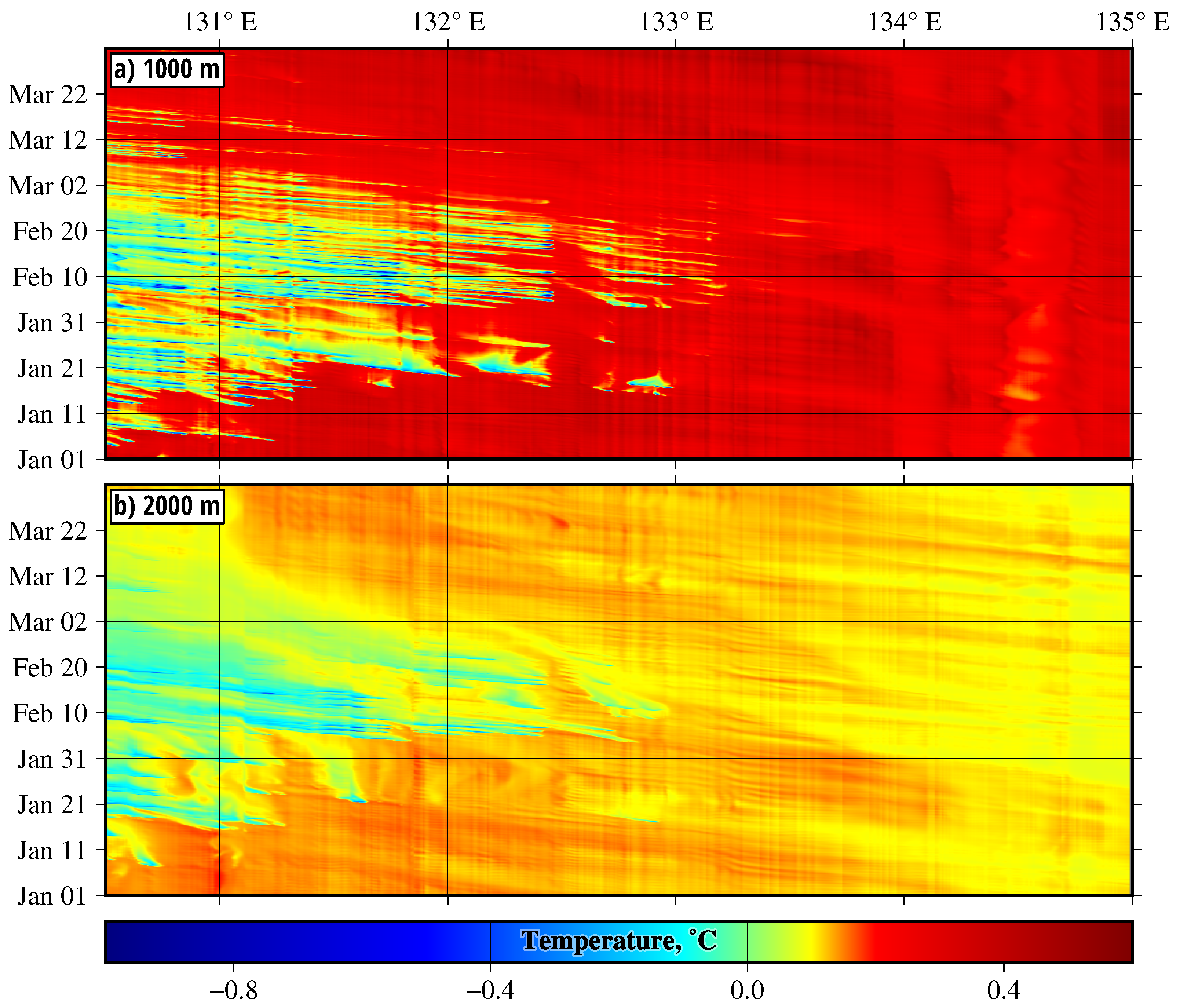
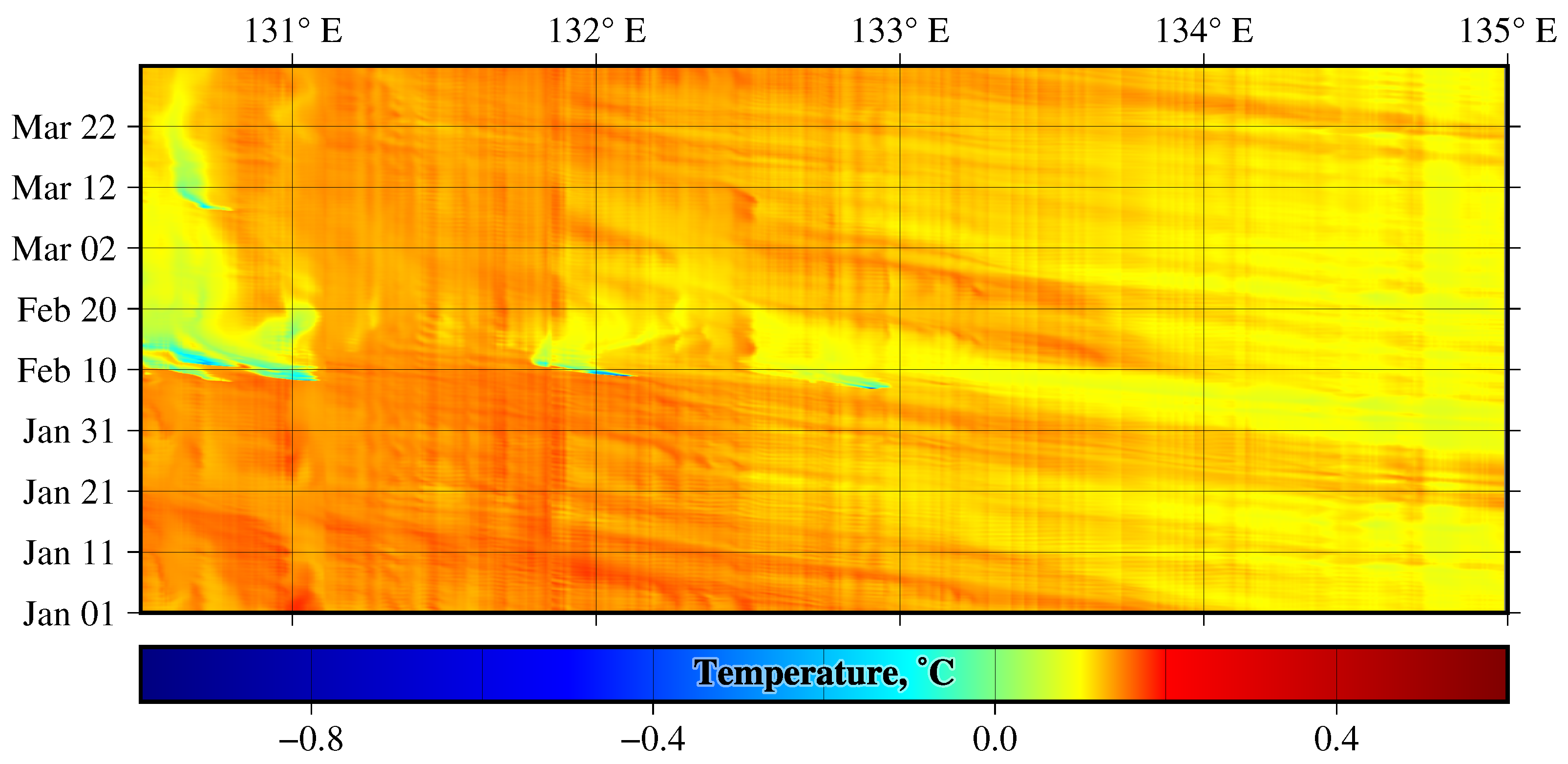
The ROMS-based simulation has shown that the descent of DSW down the slope was regularly observed from 10 January to 10 March 2001. The portions of this water mass were found to move in the bottom layer mainly from the shallow shelf of the eastern PGB (
Figure 2) to the slope edge. Some of them were advected by the Primorsky Current southwestwards, reaching depths of 2000 m and greater in the central and western parts of PGB. The tongues of the DSW with negative temperatures, propagating from east to west in January–March, are seen in the Hovmuller diagrams along the 1000 and 2000 m isobaths (
Figure 2a,b). The diagram in
Figure 2a contains a larger number of intermittent tongues of cold and warm water propagating westwards along the 1000 m isobath, as compared to the number of tongues of DSW propagating along the 2000 m isobath in
Figure 2b. Nevertheless, the DSC moves along both isobaths during the same period of time and in the same direction.
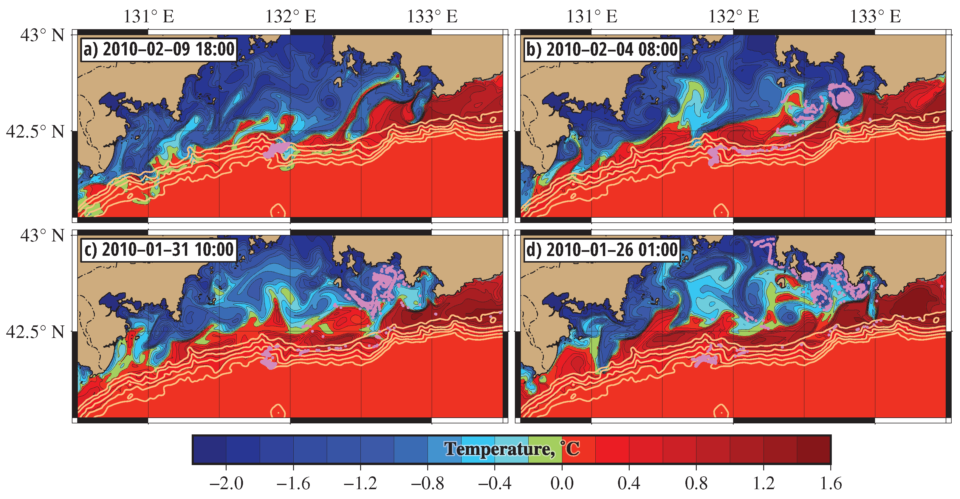
Typical distributions of temperature (T-maps) and water masses (origin or O-maps) in the bottom layer in February are shown in
Figure 3. The simulated T-map in
Figure 3a shows tongues of extremely cold DSW with temperatures reaching
°C in the shallow-shelf bottom-layer. The DSW on the continental slope at depths in the range of 1000–2000 m was warmer (between
°C and 0 °C) due to the impact of the Primorsky Current carrying warmer water. To track the paths of DSW from the shelf to the slope edge, we computed hour by hour O-maps during the whole winter of 2001, as explained in
Section 2. The DSW on the O-map in
Figure 3b and in other O-maps was defined as the water coming from the northern part of PGB. More precisely, it is the “blue” water crossing the parallel
for 30 days in the past prior to the dates shown on the O-maps. Both the T- and O-maps show the propagation of the tongues of cold DSW in the bottom layer from the shallow shelf to the slope edge in the southwestern direction. The T- and O-maps along with the Hovmuller diagrams in
Figure 2 demonstrate that the DSW descended regularly in February–March down to 2000 m. This is the first direct simulation of the phenomenon of winter DSC in PGB.
The slope convection and brine rejection in the central part of PGB were observed instrumentally from 24 February to 3 March 2001 in [
10] at the depth between 900 and 1500 m. Temperature, salinity, and oxygen content of the brine-rejected waters diverged widely from station to station, suggesting separate plumes of the original DSW as it plunged down the slope as tongues of this water shown in
Figure 3a. The potential temperature of the new bottom water was much colder than the climatological, widespread abyssal potential temperature (see
Figure 3 in [
10]). During the following spring and summer this water was observed to propagate to the south in the bottom layer with a thickness of a few hundred meters. It was characterized by an anomalously low temperature, high salinity, high dissolved oxygen, and high chlorofluorocarbon concentration overlying the deep basin off the foot of the continental slope [
7,
8].
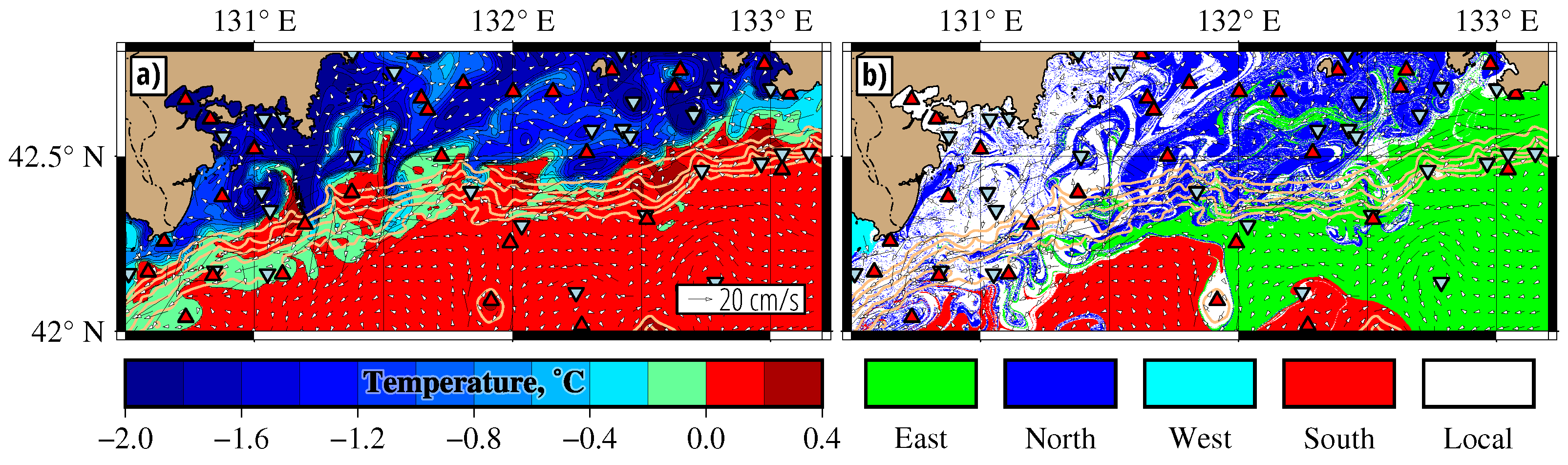
To obtain direct evidence of the DSC phenomenon, we compared our simulation results with observations made in [
10], performing numerical experiments on Lagrangian tracking of artificial passive particles launched at deep sites on the continental slope. On 23 February, many particles were placed on the section (the purple segment in
Figure 4a) where the slope convection and brine rejection were observed in [
10] at the depth between 900 and 1500 m. These particles were tracked backward in time until 3 February (
Figure 4b) when they were found to wind around a coastal cyclone centered at
,
to the south off Cape Likhachev and Vostok Bay. More integrations in time have shown that they eventually came from Vostok and Strelok Bays and from Ussury Bay (north of the
parallel).
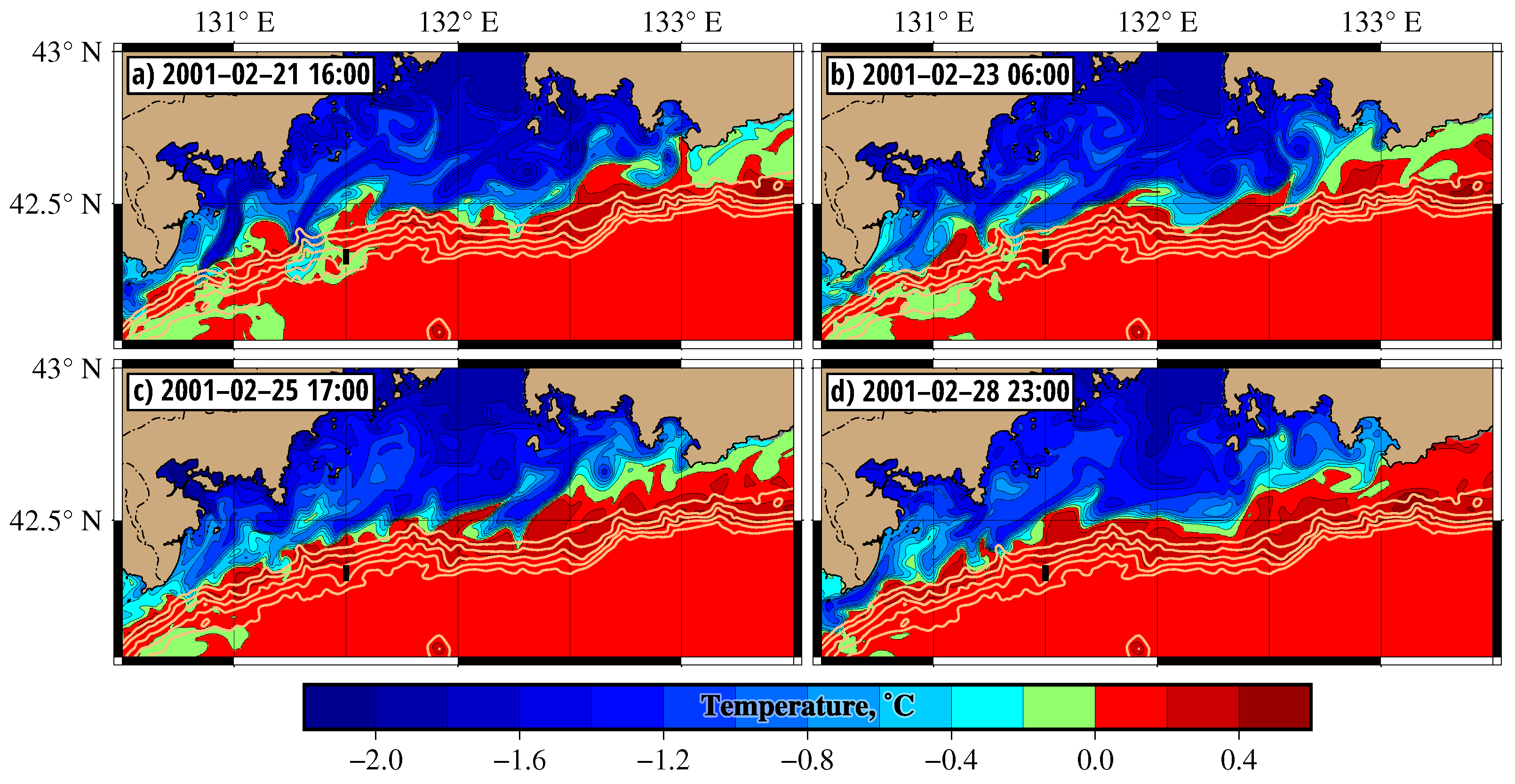
The simulated temperature maps in the bottom layer in
Figure 5 illustrate the episodes when the tongues of water with negative temperature passed the site where DSC phenomenon was observed in [
10]. The tongues of DSW move from the shallow PGB shelf to the slope edge and descend down to the depth of 2000 m and greater in the central and western PGB (
Figure 5a–d).
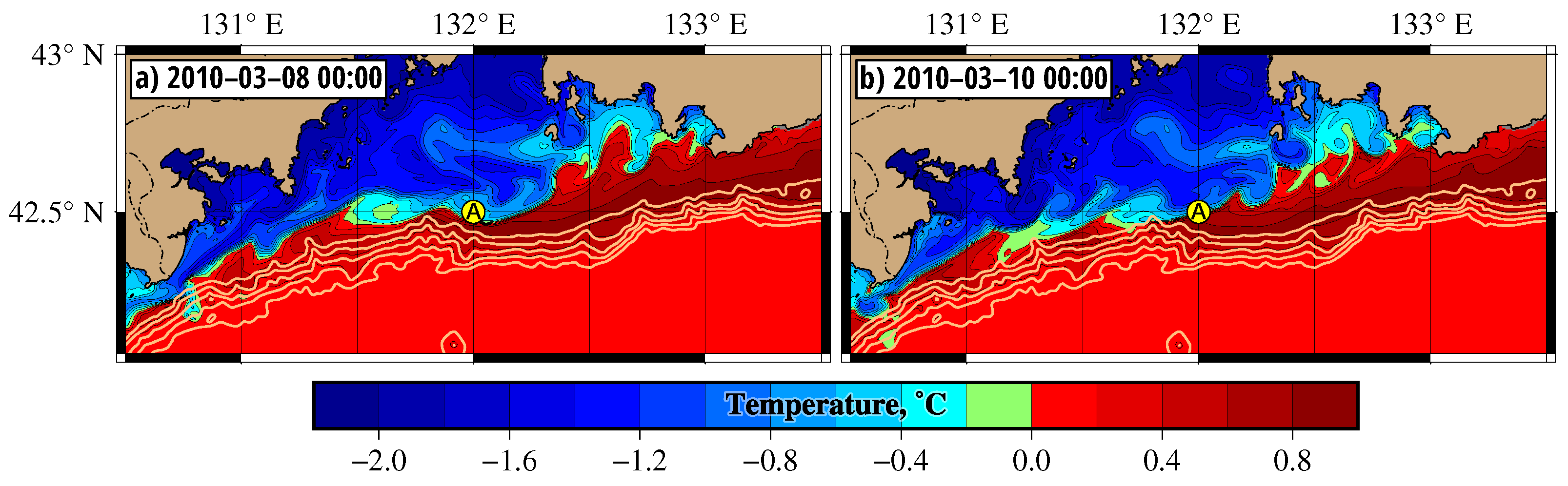
4.2. Slope Convection in Winter of 2010
Simulation for the winter of 2010 with air temperatures over PGB close to normal was chosen for comparison with the cold winter of 2001 and comparison with records of a mobile “Aqualog” profiler operated from the end of February to the middle of March, 2010 [
15]. The Hovmuller diagram in
Figure 6 shows the single episode with a DSW tongue propagating westwards along the 2000 m isobath. This tongue appeared on 9 February between
and
and reached the
meridian to 11 February. In the western part of PGB, the DSC was observed for a few days in March as a result of the descent of DSW in this area itself.
The “Aqualog” profiler [
15] was installed at the shelf break between the depths of 20 and 105 m at the point shown in
Figure 7 and
Figure 8. The buoy delivered vertical profiles of the ocean current velocity, acoustic backscatter at 2 MHz, temperature, and salinity. The depth of its location was not enough to detect the DSC phenomenon, but it was possible to record passages of DSW and compare the observation and simulated results. The DSW was recorded at the mooring site on 7 and 8 March (
°C) and 10 (
°C) (
Figure 3 and
Figure 8 in the cited paper). The simulated temperature at the “Aqualog” mooring site on 8 and 10 March in
Figure 7 agrees well with the observations. The O-maps in
Figure 8 show that the distribution of DSW and “blue” water passing the “Aqualog” mooring site during 10 and 11 February agree with the temperature distribution in
Figure 7.
5. The Role of Coastal Eddies in Cross-Shelf Transport of Dense Shelf Water
In the wintertime, cyclonic eddies regularly form in the coastal area between Askold Island and Cape Povorotny (
Figure 3,
Figure 4 and
Figure S6 in Supplementary Materials). They drift southwestwards to the continental slope and eventually decay (
Figure S5 in Supplementary Materials). In this section, we briefly discuss the role of these eddies in promoting the cross-shelf transport of DSW. The Primorsky Current flows southwestwards along the continental slope (
Figure 1), whereas DSW forms on a shallow-water shelf to the north of it.
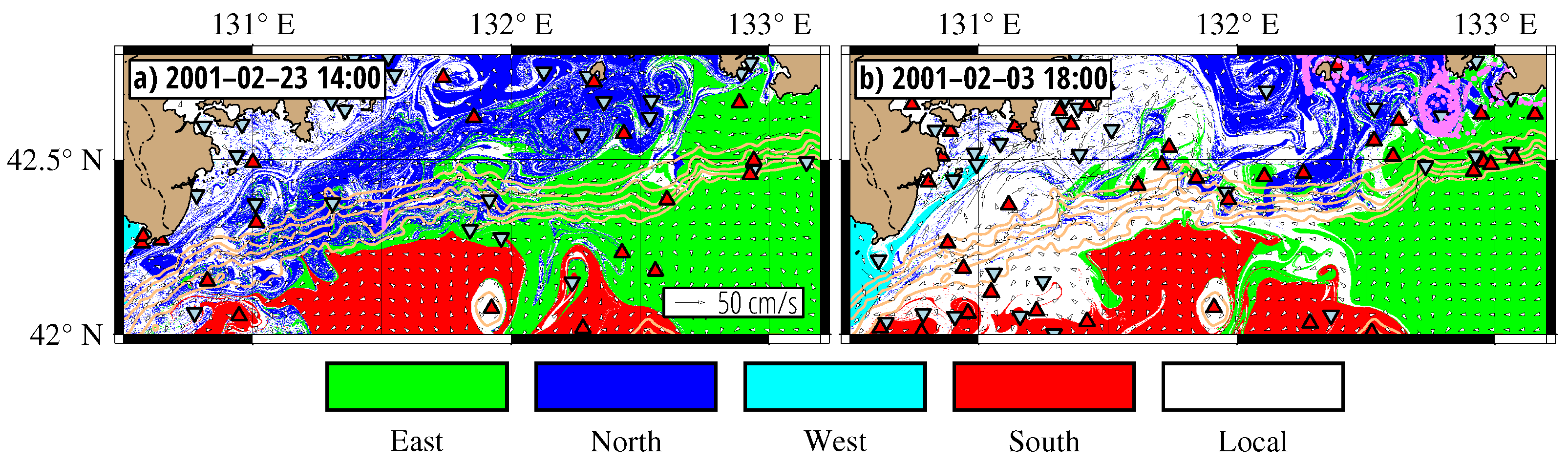
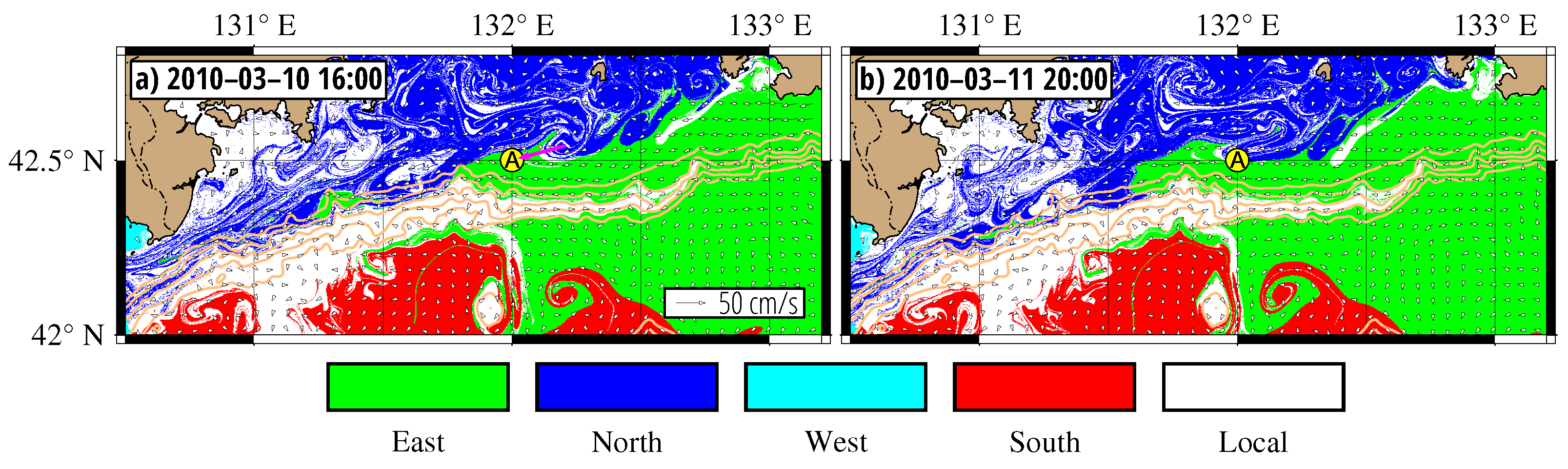
The numerical particle tracking experiment was performed to demonstrate the transport pathways of DSW from the shallow shelf to the slope edge and descent to the foot of the slope. The purple particles in
Figure 9d were launched on 16 February 2001 inside a DSW tongue at a depth between 1000 and 2000 m in the bottom layer. The particle’s trajectories were integrated backward in time to track where they came from.
As it follows from
Figure 9c, the patch preserved a compact form during 10 days after launching until it began to experience the impact of stable manifolds of the hyperbolic points shown in
Figure 9b by crosses. The locations of stable manifolds were approximated by the curves with maximum values of FTLE computed forward in time (see Equation (
3)). The FTLE map in
Figure 9, computed over 7 days, shows the distinguished stable manifolds as black curves between a cyclone centered at
,
and an anticyclone centered at
,
. The purple particles, imitating parcels of DSW in the bottom layer, spread quickly along those stable manifolds around the cyclone that worked as a kind of collector for those particles. In the first half of February, this cyclone drifted southwestwards along with the trapped DSW, eventually decayed, and released this water into the stream of the Primorsky Current, which advected this portion of DSW to the continental slope where it reached the depth of 2000 m on 16 February (
Figure 9c,d).
For comparison, we performed the numerical experiment on tracking the particles, launched on 16 February 2010 at the same place as in
Figure 9d. Over one week, the patch practically did not deform (
Figure 10a). The particles dispersed over a vast area to the beginning of February (
Figure 10b) when there existed a coastal cyclone with the center located at
,
, almost at the same place as the cyclone in
Figure 9b. This cyclone, the purple circular patch in
Figure 10b, collected the marked particles from a rather extended area (
Figure 10c,d). As in the winter of 2001, the cyclone drifted southwestwards, decayed, and release the trapped DSW into the Primorsky Current, which advected particles to the slope edge in the central PGB.
Figure 10 shows that in the regular winter of 2010, the DSW was advected to the continental slope from the same area as in the anomalously cold winter of 2001, but the events with a descent of DSW down the depth of 2000 m were very rare in the winter of 2010 (
Figure 6).
Therefore, the coastal cyclonic eddies, transporting some amount of DSW from the eastern PGB, usually drift southwestwards (
Figure S5 in Supplementary Materials) and after decay, release this water into the stream of the Primorsky Current, which, in turn, advects it to the continental slope where the DSW can reach a depth of 1000–2000 m.
6. The Role of Symmetric Instability in Generation of Coastal Cyclonic Eddies Transporting
Dense Shelf Water to the Continental Slope
Both cyclonic and anticyclonic eddies are regularly generated on the shelf of PGB. Generation of anticyclonic eddies occurs mainly in summer and has been simulated in [
31] with the same ROMS model. A short-term strengthening of the east wind led to an increase in Ekman pumping. At the same time, downwelling increased in the area of Vostok and Nakhodka bays. That led to an increase in horizontal density gradients and, as a consequence, to an instability. The instabilities eventually led to generation of long-lived anticyclonic eddies, the diameter of which can reach 100 km with the lifetime of several months. The theoretical basis for the mechanisms, by which down-front winds lead to frontogenesis, has been developed in [
32].
To find the regions in PGB with intense eddy dynamics in the cold months, we calculated the eddy kinetic energy and average that for the period from 1 January to 28 February 2001:
where
and
are mean velocity components.
Figure S6 shows areas with high values of eddy kinetic energy at different model horizons between Vostok and Nakhodka bays, south of Cape Likhachev (
Figure 1). The simulated barotropic velocity field in
Figure S7 shows that cyclonic eddies form in this region. Namely, these eddies are responsible for the transfer of cold DSW to the open part of the PGB (see
Section 6).
To find out different types of instabilities that may happen in the area between
–
and
–
, we calculated the potential vorticity, as in [
33]. The potential vorticity for continuously stratified flows is defined as follows [
34]:
where
is the buoyancy of fluid;
f, Coriolis parameter;
, density;
, current velocity;
g, gravitational acceleration. Equation (
6) can be rewritten as:
Under the assumption of a geostrophic flow (
), the thermal wind balance implies:
The geostrophic potential vorticity is then given by:
where
is the squared Brunt–Väisälä frequency,
is absolute vorticity of geostrophic flow. Equation (
9) can be separated as follows:
where
is the stratification term linked to stratification and absolute vorticity and
is the baroclinic term due to a horizontal buoyancy gradient.
Different types of instabilities can occur when the potential vorticity (
9) takes the sign opposite to that of the Coriolis parameter (i.e., negative in the northern hemisphere). It happens if:
, gravitational instability;
and , inertial or centrifugal instability;
, symmetric instability;
, and , inertial/symmetric instability;
and , symmetric/gravitational instability.
Visual inspection of the velocity field showed that eleven cyclonic eddies formed in the study area from 21 January to 20 February 2001. As an example, let us consider a cyclonic eddy that appeared on 29 January and analyze how the velocity field changed hour by hour during that day and preceding days (
Figure S7 in Supplementary Materials). For analysis, it is convenient to consider the barotropic component of velocity and the vertical section of temperature along
. During 28 January, a strong northwesterly wind blew over the study area with a speed of up to 12 m/s. This caused an intensification of the southward flow along the eastern coast of Vostok Bay. The potential vorticity in the study area was positive. By the end of 28 January, this flow transported cold DSW to the southern tip of Cape Likhachev. By 02:00 on 29 January, horizontal density gradients increased in the coastal zone, and the potential vorticity became negative because the absolute value of baroclinic term became larger than the stratification term. This led to the symmetric instability and generation of a cyclonic eddy near the coast (
Figure S7 in Supplementary Materials). The conditions for existence of the symmetrical instability was maintained for two hours. During this period of time, the cyclonic eddy gradually increased in size. After 04:00, the negative relative vorticity became greater in absolute value than the planetary one, and the absolute vorticity became negative. This led to the inertial/symmetric instability. In the second half of 29 January, the diameter of the cyclonic eddy reached the value of 10 km and began to move to the west entraining DSW.
7. Conclusions
Every winter, dense shelf water (DSW) builds up on the PGB shallow shelf until it occupies the entire depth. The density of DSW is about the same as the density of the surrounding waters in the bottom layer. The isobaths, along which this water spreads in depth, depend on atmospheric conditions. Usually the DSW does not descent below 1000–1200 m. However, in extremely cold winters the density of this water can be so large that it is able to sink down to 2000 m and even deeper, mixing with waters of the same density [
7,
8,
10].
Using ROMS with a spatial resolution of 600 m, we performed numerical experiments to simulate the main stages of the deep slope convection (DSC) in PGB in the anomalously cold winter of 2001. Computing hourly Lagrangian origin maps, we tracked the propagation of the DSW in the bottom layer from the shelf to the slope edge that occurred in the form of tongues of water with a negative temperature. Some of these tongues have been found to descent regularly down to the depth of 2000 m and greater. The origin and temperature maps allowed us to document hour by hour the phenomenon of DSC, including the formation of DSW, the cross-shelf transport towards the continental slope edge and descent down the slope. We have shown that the DSC regularly occurred from the middle of January to the beginning of March in 2001. The simulation results on Lagrangian tracking of artificial particles have been found to agree qualitatively with shipboard observations [
10] in the end of February 2001. The simulation has also been performed for the regular winter of 2010 when hydrological characteristics of DSW were recorded by a profiler “Aqualog” installed at the shelf break in PGB [
15]. In this winter, the descent of DSW down to 2000 m was found only once.
It was shown that the symmetric instability can occur in the coastal area of the eastern PGB causing the generation of cyclonic eddies with a size of 10–20 km, which promote the cross-shelf transport of DSW. These coastal eddies were found to collect portions of DSW in the core and around the periphery. They usually drift southwestwards and, after decay, release this water into the stream of the Primorsky Current which, in turn, advects it to the continental slope where DSW can reach great depths in the central and western PGB.


 ,
, 