Abstract
The microfluid jet polishing (MFJP) process is a manufacturing technology in which small abrasive particles (such as diamond, alumina, and ceria) are premixed with a carrier fluid (typically water) to form a liquid suspension that is pressurized and expelled through a nozzle for material removal. The resulting microjet beam—with a typical nozzle exit diameter in the range from 0.1 to 1.0 mm—impinges the workpiece surface for material removal by erosion and/or abrasion and produces an ultraprecision surface. This work applies a computational fluid dynamics (CFD) model to analyze the key phenomena in the interaction of the liquid suspension and the workpiece surface. The liquid film characteristics (film height, minimum film height, positions of the minimum film height, and hydraulic jump) obtained from the CFD simulations are compared with the results derived from empirical formulations found in the literature. Subsequently, the numerical results are utilized to investigate the impact velocity, pressure distribution, and shear stress caused by the suspension on the workpiece surface. It is observed that the shear stress strongly depends on the injection pressure of the liquid suspension and is weakly dependent on the abrasive suspension concentration (the liquid suspension with different densities, viscosities, and surface tensions). Additionally, the particle behavior is investigated in order to estimate the impact velocity and to identify the impact and erosion zones of the liquid suspension on the workpiece surface. Numerical results indicate that ~50% of total particles are impinging the workpiece surface almost perpendicularly (with a mean impact angle of ~86 degrees) for the first time in the stagnation region, where they are strongly decelerated by the carrier fluid before they reach the workpiece surface. These particles, however, rebound on the surface and are reaccelerated by the carrier fluid, impinging the workpiece surface further in the radial direction.
1. Introduction
The development and mastery of finishing processes for creating high-precision optical surfaces are challenging. The fabrication of high-precision optical surfaces generally involves several processing steps, including milling [1], grinding [2], polishing [3], and final finishing. Fluid jet polishing (FJP) [4,5] is a machining process in which abrasives (ceria, alumina, silicon carbide, or diamond particles with a diameter < 10 µm) and a carrier fluid (typically water) are adequately premixed and pumped through a nozzle. The resulting jet beam impinges the working surface either perpendicularly or at an impingement angle, allowing individual abrasive particles within the carrier fluid to impact the workpiece surface. The release of the kinetic energy of the abrasive particles results in variable material removal rates through the control of process parameters [6,7,8]. FJP is an ultraprecision finishing technology that merges fluid dynamics, precision manufacturing, and surface engineering, and has high adaptability to be applied for generating complex free-form shapes [9] and the ultraprecision polishing of optical lenses, mirrors, and molds [10]. Figure 1 presents a sketch of the FJP process. The material removal mechanisms are influenced by several process parameters and material characteristics, as shown in Figure 2.
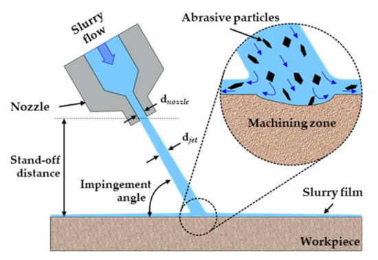
Figure 1.
Sketch of the fluid jet polishing process.
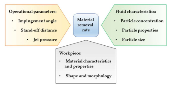
Figure 2.
Main factors affecting the material removal rate in the FJP process.
In the recent past, several experiments have been performed in order to derive the fundamentals of the process. Fähnle and coworkers [5,8,11,12,13,14] investigated the material removal and optimized the polishing process of the optical lenses. Beaucamp and coworkers [10,15,16,17] introduced different techniques together with the FJP process to increase the material removal rate without causing any significant deterioration on the surface finishing. Wang et al. [18] proposed a multijet polishing method to enhance the polishing efficiency. Wang et al. [9] investigated the influence of different stand-off distances (SOD) on the characteristics of the resulting workpiece surface quality. Li et al. [19,20] studied the tool influence function (TIF) of the FJP and applied the process to remove the tool marks left on the workpiece single-point diamond turning.
Microfluid jet polishing (MFJP) (a derivation of the FJP technique) has been applied as a finishing process to produce high-precision surfaces [15,21,22,23] such as optical lenses and molds of different materials. However, the understanding of the fundamental process characteristics is far from complete, and some fundamental mechanisms still need to be addressed, especially the effects of the hydrodynamics and fluid flow behavior on the removal rate of the material, as the fluid properties and its interaction with the workpiece surface are the key factors of the performance of the MFJP process. In this sense, computational fluid dynamics (CFD) is a powerful tool to provide deeper insights into the investigations of several multiphase flow systems [24,25,26,27,28,29,30,31] because several aspects of the physical phenomena occurring at different time and length scales can be acquired. Nguyen et al. [32] investigated the jet flow characteristics and the erosion of a workpiece surface of a water–sand multiphase flow via a combined numerical–experimental approach. The authors investigated the behavior of particles with a mean diameter of 150 µm impinging on a workpiece submerged in a water tank. Cao and Cheung [22] applied an erosion model to investigate the erosion rate of the FJP process with a monodisperse particle distribution. Qi et al. [33] analyzed the behavior of the monodisperse particles with diameters of 3, 9, and 15 µm in a multiphase flow slurry jet. Qi et al. [34] performed numerical investigations of ultrasonic-assisted abrasive jets with glass particles having a mean diameter of ~10 µm. Wang et al. [18] combined numerical and experimental investigations of a multijet polishing process in order to study the erosion rate of the workpiece surface. The authors compared different multijet configurations and compared the results with a single-jet configuration. Although several studies are found using CFD techniques to investigate the multiphase flows applied to the FJP process, most previous numerical studies either use large particles or consider the monodisperse distribution of the particulate material.
In this work, the fundamental analysis of a fluid jet impacting a surface is performed using a Eulerian–Eulerian approach in a two-dimensional (2D) domain. The numerical results obtained from the CFD simulations of the fluid suspension are compared with results obtained from empirical/algebraic equations. The numerical geometry is extended to a three-dimensional (3D) domain, and the particle behavior with a size distribution under 10 µm (Sauter mean diameter of ~1.4 µm) is investigated using a Eulerian–Eulerian–Lagrangian approach to predict the behavior of the gas, liquid suspension, and abrasive particulate phases, respectively.
2. Empirical and Algebraic Approximations of the Fluid Film Behavior
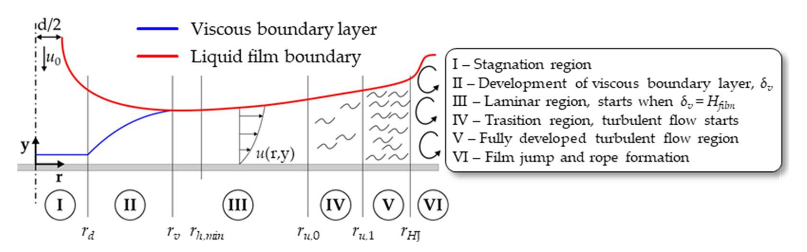
Figure 3 presents a sketch of different flow structures occurring in a perpendicular impinging liquid jet in a gaseous atmosphere. The flow field can be divided into several regimes. Near the impacting point on the workpiece surface, the fluid flow is described as the stagnation region, where the viscous boundary represents a constant value disregarding the distance to the jet center on the workpiece.
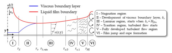
Figure 3.
Sketch of the different flow regimes of the liquid film on the workpiece surface (not to scale). (Adapted with permission from [35]. Copyright 2022 ASME INTERNATIONAL).
The pressure in the stagnation region, , can be estimated by applying the Bernoulli equation [36] as follows:
where is the ambient pressure, is the constant liquid phase density, and is the liquid velocity at the exit of the nozzle. In the stagnation region, the velocity direction changes from a perpendicular profile to a parallel profile against the workpiece surface. The flow conditions on the workpiece surface or directly above the boundary layer are described with the dimensionless gradient B [37]:
For the radial position (considering the jet axis as ) with the dimensionless gradient (Equation (2)), it is possible to estimate the velocity and pressure as a function of the radial position:
where is the nozzle diameter. Assuming the hypotheses of the uniform velocity profile of circular jets, for which the dimensionless velocity gradient B is equal to 1.832 [37,38], the overpressure distribution in the stagnation region can be derived from Equation (4) as:
From a dimensionless radial position of approximately , the overpressure is almost zero, and the film velocity is close to the fluid velocity at the nozzle exit [36]. Up to a radial position , the thickness of the viscous boundary layer remains constant. According to Ma et al. [39], the thickness of the viscous boundary layer, , can be described as:
where is the Reynolds number of the fluid jet flow calculated at the nozzle exit, defined by:
where is the liquid viscosity. The mean radial velocity of the fluid film can be derived from the continuity equation, i.e., from the radial position and the thickness of the fluid film. Outside the stagnation region, the fluid flows parallel to the workpiece surface, and its velocity decreases due to the friction effects [40]. In the near of the stagnation region, the fluid film thickness decreases with the increase of the radial distance until it increases again in the posterior radial distance due to the friction effects and the associated velocity reduction. According to Watson [41], the fluid film thickness is described as:
The mean velocity of the fluid film can be estimated as:
Away from the stagnation region, the viscous boundary layer increases with increasing the radial distance (region II) until it reaches the fluid film surface (the gas–liquid interface). According to Lienhard [37], the radial position, , where the viscous boundary layer reaches the fluid film surface, is described as follows:
Additionally, the thickness of the viscous boundary layer and the fluid film height can be described as a function of the Reynolds number and the radial position as:
The radial flow of the liquid fluid in this region (II) generates a wall shear stress , which can be described as [36]:
A laminar flow profile is observed in the following region (III), where the minimum film height is observed. In this region, the fluid velocity decreases with increasing the radial distance from the centerline of the jet where the thickness of the viscous boundary layer is equal to the film height, . According to Lienhard [37], the fluid velocity at the film surface (gas-liquid interface) is described as:
where the fluid film height is a function of the radial distance:
The wall shear stress in the laminar region can be expressed as follows:
In the laminar region, the minimum thickness of the fluid film is found. According to Bhagat and Wilson [36], the radial position of the minimum film is described as:
After that, a transitory behavior (region IV), followed by a fully developed turbulent flow (region V), is observed. The transition region starts at and ends at , after which the fully turbulent flow region starts (see Figure 3). According to Liu et al. [35], these two positions are described as follows:
The thickness of the fluid film increases after the laminar region. This increase in the fluid film height is attributed to the formation of turbulence. In these regions (IV and V), the boundary layers quickly reach the free surface of the fluid film due to the turbulence. The thickness of the fluid film in these regions can be described as:
In the turbulent flow region (), the wall shear stress can be estimated with the Blasius approach [42], resulting in:
In the fully turbulent region, the velocity profile can be described by a 1/7th power distribution [43] as a function of the liquid viscosity and the film surface velocity (gas–liquid interface) as follows:
Further downstream of the fully turbulent region, the velocity of the fluid flow decreases until it is equal to the wave propagation velocity, and a wave crest, the so-called hydraulic jump, forms (region VI in Figure 3). At the position where the hydraulic jump forms, the gravitational and inertial forces cancel each other. The ratio of such forces is described by the dimensionless Froude number, . When the critical Froude number, , is achieved, the hydraulic jump arises:
where is the acceleration due to gravity. In practice, the origin of the hydraulic jump differs due to the surface roughness and disturbances within the fluid flow and occurs when the momentum per unit circumferential width is equal to the surface tension. According to Baonga et al. [44], the radial position of the hydraulic jump can be described as a function of the Reynolds number with a maximum uncertainty of 2%, as follows:
The values of velocity, pressure, viscous boundary layer and liquid film thickness, and wall shear stress can be calculated from the presented empirical equations, which are mainly based on experimental results and serve as validation to the numerical results from the CFD simulations.
3. Numerical Setup
Different kinds of mathematical modeling, such as the Reynolds-averaged Navier–Stokes equations (RANS), large-eddy simulations (LES), or direct numerical simulations (DNS) and numerical discretization techniques, including the finite element method (FEM), finite volume method (FVM), lattice Boltzmann method (LBM), and immersed boundary method (IBM), can be applied to predict and investigate the FJP process. This section describes the mathematical approaches, numerical methodology, and operating and boundary conditions used in this work.
3.1. Geometry and Numerical Domain
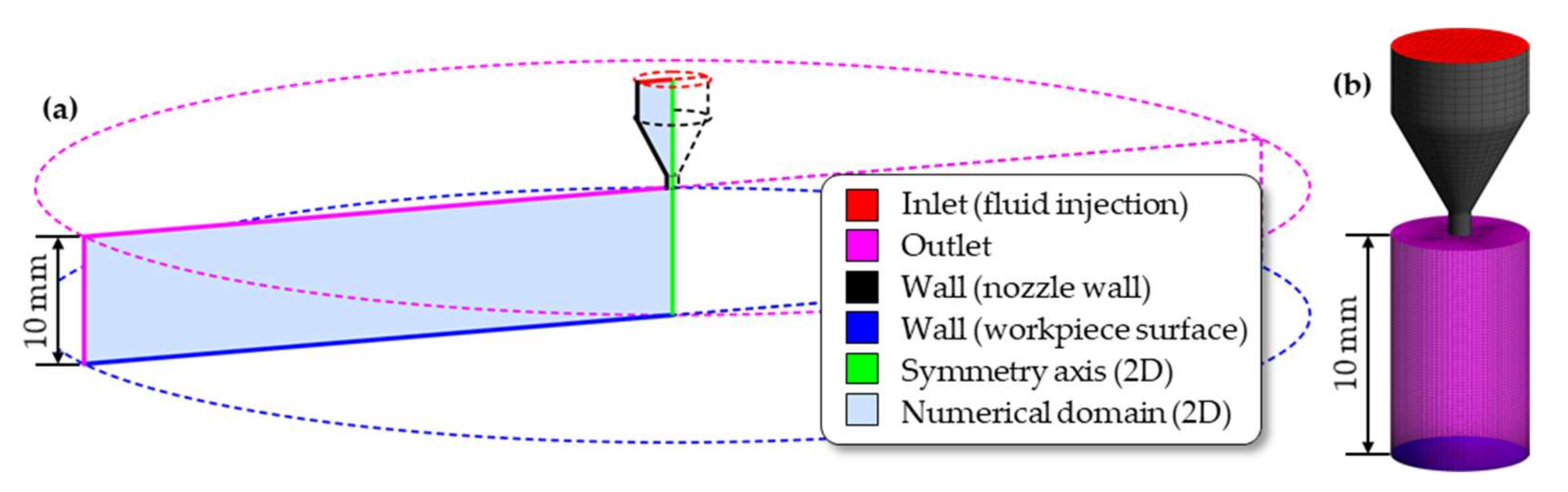
The numerical geometry of the microfluid jet polishing process consists of a nozzle with an inner diameter of 1 mm, positioned perpendicular (in this work) to a surface with a stand-off distance of 10 mm. In this study, the surface is positioned horizontally, and the fluid jet flows in the top-to-bottom direction. Two different numerical domains are applied, namely a 2D domain in an axisymmetric approach (Figure 4a) and a fully 3D domain (Figure 4b). In the 2D numerical domain, the radius of the axisymmetric domain is 50 mm (a workpiece surface with 100 mm in diameter) while, in the 3D numerical domain, only the region near the jet impingement zone is considered (a domain diameter width 6 mm). The 2D domain consists of ~143,000 cells, while the 3D domain has ~276,000 cells.
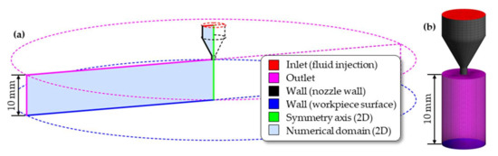
Figure 4.
Numerical domain of the (a) 2D axisymmetric approach and (b) fully 3D domain of the FJP process.
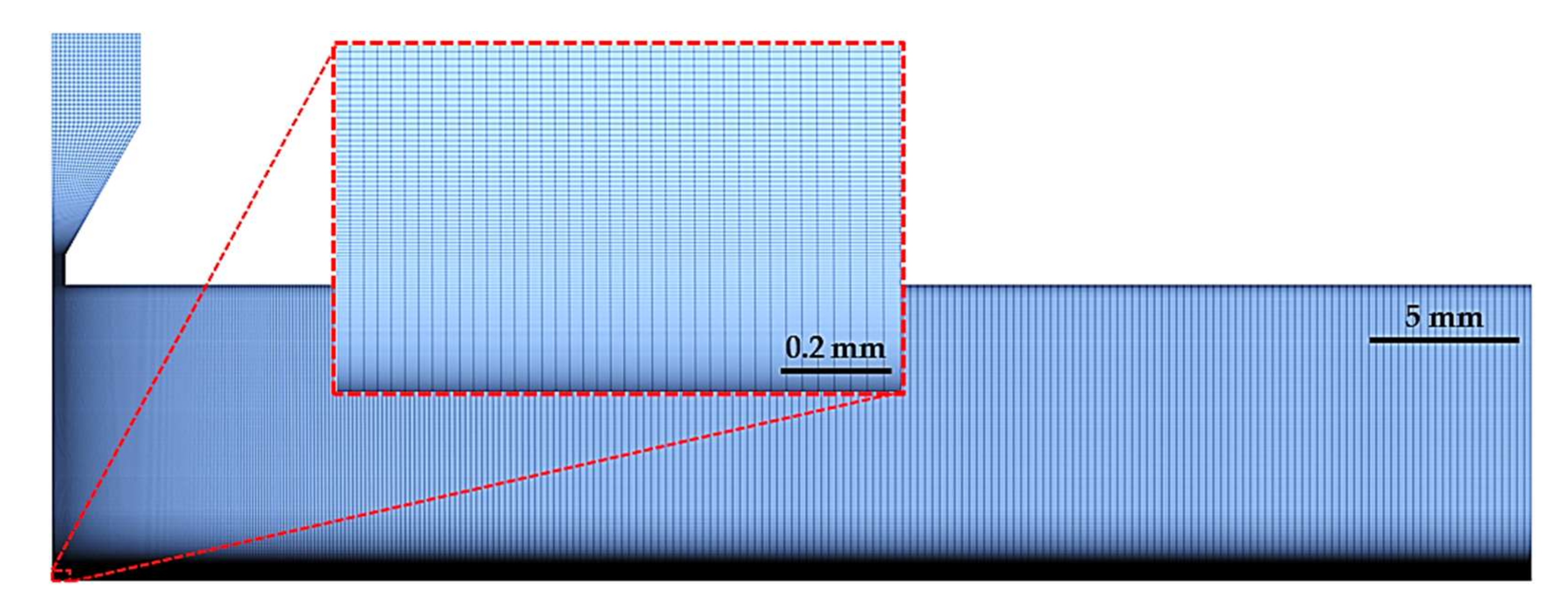
In the 2D approach, the computational mesh is made of quadrilateral elements, while in the 3D domain, the mesh is constructed with hexahedral elements. In both approaches, the mesh is refined in the region near to impinging zone, where high velocity and pressure gradients are observed. Additionally, a good mesh resolution at the boundary layer is necessary to obtain high-quality numerical results. The minimum number of cells to predict the boundary layer accurately is ~10 [45]. In the present work, the number of cells at the position of the minimum film thickness is ~25 in the wall-normal direction. The first cell layer has a thickness of 1 µm with a mesh growth rate of 1.02 from the wall surface in the wall-normal direction. Details of the mesh resolution (2D domain) are presented in Figure 5. The 3D domain has a similar resolution to the 2D approach. The 2D domain is applied to compare and validate the results of the fluid flow hydrodynamics obtained by the CFD simulations with the empirical correlations presented in Section 2, whereas the 3D domain is used to investigate the particle behavior in the impinging region.

Figure 5.
Mesh resolution of the 2D domain with detail of the impingement region.
3.2. Mathematical Modeling
The mathematical model and numerical methods applied in the present study consider the gas (air) and liquid (liquid suspension) phases as continuum fluids and the abrasive particles as a discrete phase in a Eulerian–Eulerian–Lagrangian (EEL) framework under steady-state conditions and incompressible flow. The transport of the averaged fluid flow quantities is modeled by the RANS equations assuming the eddy viscosity hypotheses. To close the RANS equations, the turbulent correlation for the Reynolds stresses should be modeled. For the turbulence modeling, the shear-stress transport (SST) k–ω model [46], which is based on a blend of the k–ε and k–ω models, is applied to express the turbulent fluid flow in the inner and in the outer parts of the boundary layer for a wide range of the Reynolds numbers. The modified formulation for the turbulent viscosity, µt, is calculated by the SST k-ω model as a function of turbulence kinetic energy, k, and specific dissipation rate, ω.
The volume of fluid (VoF) formulation is applied as the multiphase model to describe the evolution of the interfaces between the gas and liquid phases [47]. The volume fraction of the liquid suspension is defined as βL. When the cell of the numerical domain is full of the liquid phase, βL = 1. When the cell is full of air, βL = 0. When the cell contains the liquid and the gas phase interfaces, 0 < βL < 1. In the present study, there is no mass transfer between the liquid and gas phases, therefore, no new source term needs to be specified.
To estimate the detailed information of the particle dynamics into the fluid flow, the discrete phase model (DPM) is applied. Two-way coupling between the continuous and discrete phases is applied. In a fluid-particle flow, particle–particle interactions can play an important role. According to Crowe et al. [48], a qualitative characterization of the dilute or dense nature of a fluid-particle flow can be made by estimating the ratio of the characteristic interparticle collision time τC between the particles to the particle relaxation time τP. The interparticle collision time and the particle relaxation time are described as:
where is the particle diameter, is the number density of particles, is the mean fluctuation velocity of particles, and is the particle density. If the ratio τC/τP < 1, the fluid-particle flow is particle–particle collision-dominated and the particle–particle interactions need to be considered. In this study, the ratio τC/τP ≫ 1, meaning that the time between adjacent particle–particle collisions is too large, allowing the particle to be accelerated by the aerodynamic forces of the carrier fluid before the next particle–particle collision occurs. Therefore, in this work, particle–particle are assumed to be negligible.
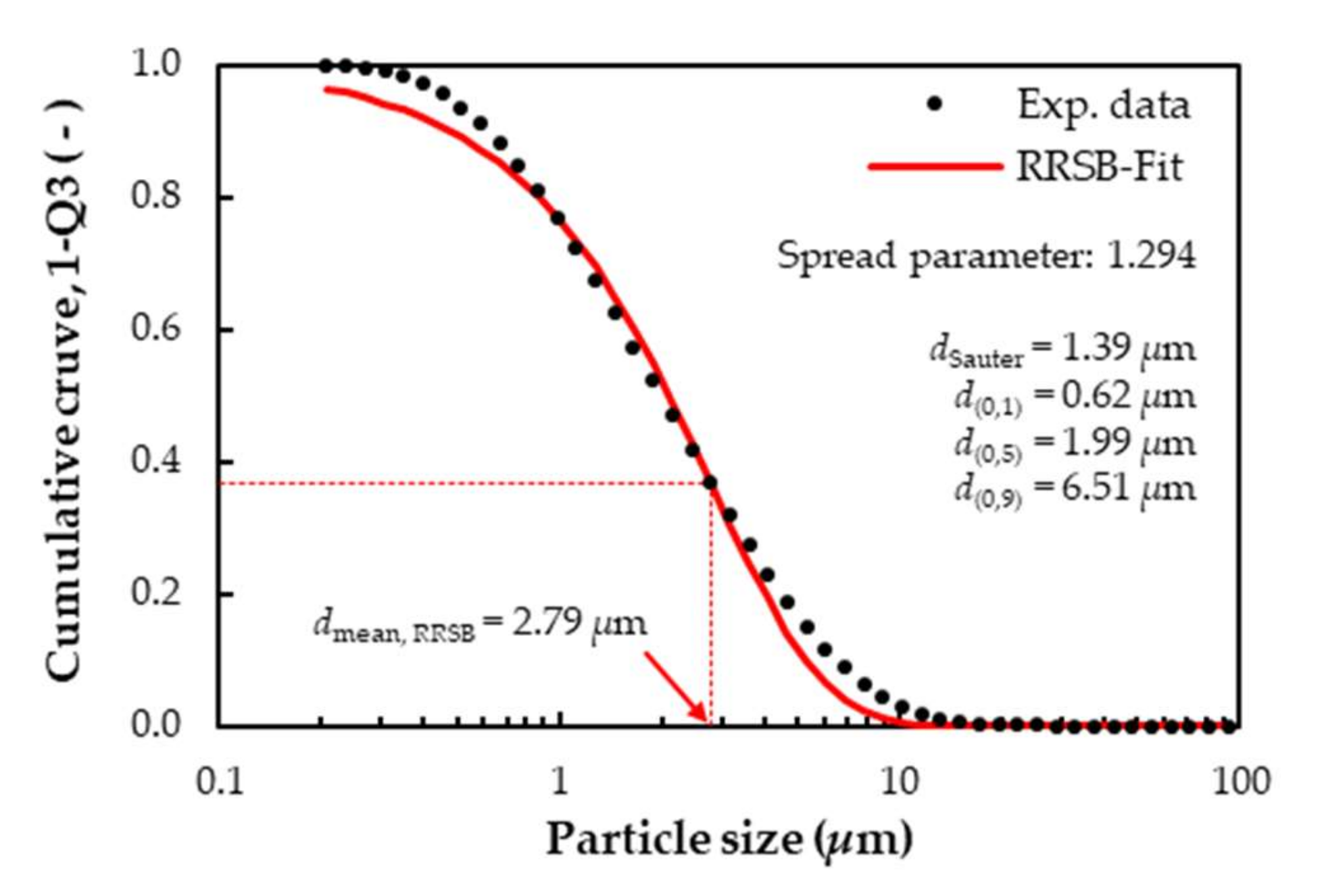
The effect of the fluid turbulence on the particle motion is considered using the stochastic discrete walk (DRW) model [49], in which the velocity fluctuations are included in the integration of the particle trajectories of each particle. The drag force on the particles is considered with the drag force model coefficient from Morsi and Alexander [50]. Proper particle size distribution is obtained from experimental measurements and correlated with a Rosin–Rammler–Sperling–Bennet (RRSB) function [51,52,53] to obtain the mean particle diameter, dmean,RRSB, and the spread parameter factor, which are applied as relevant parameters for the model setup. The RRSB parameters and the relevant particle information are presented in Figure 6.
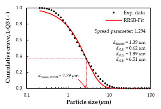
Figure 6.
Experimental data of CeO2 particle size distribution; black dots are measured data and the red line is the fitted RRSB distribution function.
3.3. Numerical Methodology
The partial differential equations (PDE) of the mathematical model are computed utilizing the finite-volume method (FVM). A pressure-based and implicit coupled solver is applied to solve the pressure–velocity coupling and second-order spatial discretization under steady-state conditions. The convergence solution is achieved when all the normalized residuals of the flow variables decrease at least three orders of magnitude and variable values remain stable. The ANSYS Fluent v.20.0 code is utilized in all the simulations.
Regarding the mesh quality, a grid independence study is performed using the grid convergence index (GCI) method presented by Celik et al. [54] as a recommended procedure for reporting the uncertainty due to numerical discretization. Three different structured mesh schemes were analyzed with a refinement ratio of ~1.45 between the meshes. A representative cell size, h, has been computed for each mesh by dividing the entire fluid domain by the corresponding number of cells. The operating condition with a pressure drop of 0.6 MPa was applied to the grid convergence analysis. Two variables, maximum liquid velocity and maximum wall shear stress, were considered to estimate the discretization error. The main parameters calculated with the GCI procedure are presented in Table 1.

Table 1.
Variables and respective values considered for the GCI analysis and calculated discretization errors.
According to Table 1, the numerical uncertainty with the refined grid resolution is less than 0.49% (approximated relative error). The maximum tangential velocity presented values of 33.04 m/s, 33.91 m/s, and 34.08 m/s for the coarse, intermediate, and fine meshes, respectively, while the maximum wall shear stress obtained from the different mesh refinement was 5.09 kPa, 5.21 kPa, and 5.24 kPa (coarse, intermediate, and fine meshes, respectively). The extrapolated value (when h→0) of the maximum tangential velocity and maximum wall shear stress are 34.11 m/s and 5.25 kPa, respectively, leading to a GCI of 0.17%.
To ensure the grid refinement is sufficient, the solution must be in an asymptotic range, i.e., the analyzed variable (in this case, the maximum tangential velocity and wall shear stress) should converge to a single value with the grid refinement. Figure 7 shows the plot of this quantity as a function of the representative cell size of each mesh. As visible in Figure 7 (and presented in Table 1), the maximum tangential velocity and maximum wall shear stress with the most refined mesh (34.08 m/s and 5.24 kPa) are very close to the values of the extrapolated maximum tangential velocity and maximum wall shear stress (34.11 m/s and 5.25 kPa). Furthermore, the orthogonality and the aspect ratio of the cells are evaluated, presenting values of >0.95 and >0.5, respectively, for over 95% of the elements. Therefore, the corresponding grid resolution is adequate for the simulations.
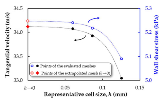
Figure 7.
Qualitative representation of the grid convergence study.
3.4. Operating and Boundary Conditions
The liquid suspension is injected with different mass flow rates according to the different pressure drop applied and the particle concentration in the suspension. Liquid suspensions with different properties (fluid viscosity and density) due to the particle concentrations are investigated. The introduction of a solid phase lacking internal fluidity into a liquid reduces the overall fluidity and therefore increases the viscosity of the particle–liquid composite system in comparison with the pure liquid [55]. For diluted particle suspension (particle volume concentration ), the Einstein equation [56,57] for viscosity estimation can be applied. The evolution of the fluid viscosity and density due to the particle concentration in the liquid suspension is presented in Figure 8.
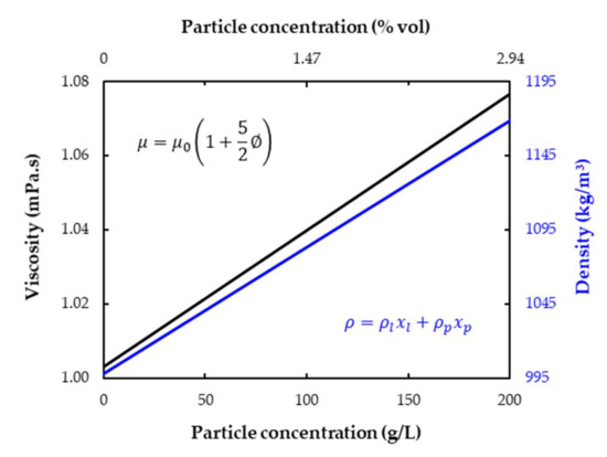
Figure 8.
Variation of the viscosity and density of the liquid suspension due to the particle concentration; the liquid viscosity is calculated with the Einstein equation.
The fluid density is proportional to the mass fraction of the liquid and particles in the suspension. The Einstein equation is presented as:
where is the viscosity of the pure liquid and is the volume concentration of the solid dispersed particles. The assumptions for the Equation (27) are that the liquid phase is Newtonian, the solution is diluted (), and the solid particles are spheroids [55]. The particles under investigation are cerium oxide (CeO2—Super Cerox 1663 TM) with the diameter ranging from ~0.2 to ~25 µm with a Sauter mean diameter dSauter = 1.39 µm (see Figure 6), resulting in a Stokes number St in the order of ~0.03 (Figure 9b):
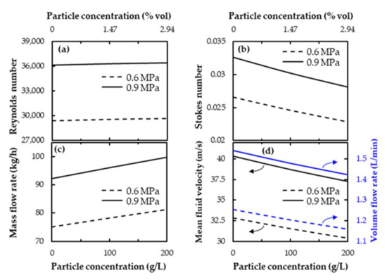
Figure 9.
Variation of (a) Reynolds number, (b) Stokes number, (c) liquid mass flow rate and (d) liquid velocity at the nozzle exit (black lines), and liquid volume flow rate (blue lines) due to different inlet pressure (0.6 MPa in dashed lines and 0.9 MPa in solid lines) and particle concentrations.
The main operating and boundary conditions are presented in Table 2 and Table 3, respectively. As shown in Figure 8, the particle concentration modifications lead to changes in the fluid viscosity and density. These changes affect the Reynolds number, as they modify the volume and mass flow rates and, consequently, the mean velocity of the fluid at the nozzle exit. Additionally, modifying the inlet pressure also changes these values mentioned above. Figure 9 illustrates the variations of operating conditions due to changes in the particle concentration and inlet pressure of the liquid suspension.
Table 2.
Operating conditions adopted in the numerical setup.
Table 3.
Boundary conditions adopted in the numerical simulations. The mass flow rate of the liquid suspension injected at the boundary “Inlet” depends on the inlet pressure and particle concentration (See Figure 9c).
The changes in the particle concentration have a low influence on the Reynolds number (Figure 9a) since the viscosity and density of the fluid change almost proportionally with the increasing concentration (Figure 8). However, the Reynolds number changes significantly by varying the inlet pressure, from Re ≈ 29,000 at 0.6 MPa to Re ≈ 36,000 at 0.9 MPa. On the other hand, the mass flow rate of the fluid increases with increasing both the particle concentration and the inlet pressure (Figure 9c) while the mean flow velocity (at the exit of the nozzle) and volume flow rate of the fluid (Figure 9d) decrease.
4. Results and Discussion
The effect of different particle concentrations of the fluid suspension and different operation pressures on the fluid behavior, fluid–workpiece interactions, and fluid–particle dynamics are investigated using CFD techniques. To validate the mathematical approach, a comparison with results of empirical/algebraic formulations is performed in terms of the fluid behavior, namely the fluid film and viscous boundary layer thickness and different radial positions where different phenomena occur inside the fluid flow. This validation is performed by using a 2D axisymmetric approach. Additionally, a fully 3D domain is applied to investigate the particle behavior in the regions close to the impingement zone.
4.1. Fluid Flow Behavior
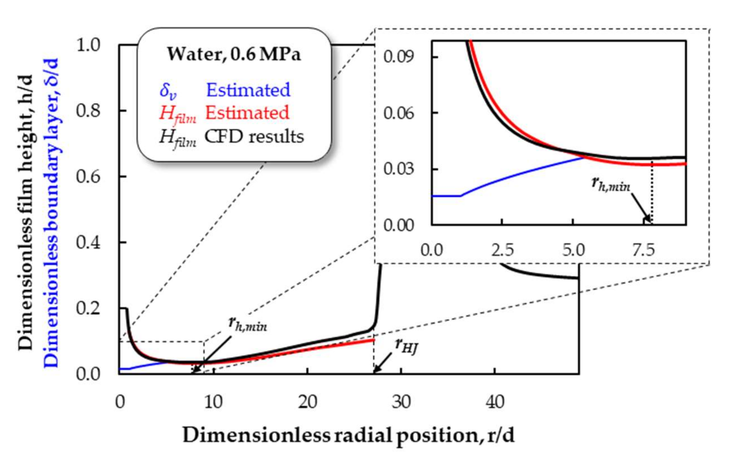
This section presents the results of velocity and pressure fields from the numerical simulations with different particle concentrations in the fluid (variation of fluid viscosity and density) and different inlet pressure. Figure 10 presents a comparison of the film thickness and boundary layer thickness (in nondimensional form) between the results obtained with the empirical/algebraic equations from Section 2 and the numerical results from the CFD simulations for pure water with an inlet pressure of 0.6 MPa. A good agreement is observed in the region near the impingement zone (up to r/d < 10). A slight divergence in the liquid film thickness is observed in the region further away from the impingement zone. At r/d = 25, the divergence is ~10% (absolute difference between both results). This divergence can be attributed to the way that the film thickness is estimated: with the empirical/algebraic approach (Equations (8), (12), (15) and (20)), the film thickness is estimated based on the Reynolds number of the fluid at the nozzle exit, while in the CFD approach, the film thickness is predicted by the local fluid properties. Additionally, the liquid film thickness is considered in the interface of the gas-liquid flow when the volume fraction of the liquid phase in the cell βL > 0.7. The radial position where the minimum liquid film thickness and the hydraulic jump occur are very similar in empirical and numerical results.

Figure 10.
Comparison between numerical and empirical formulation results to estimate the viscous boundary layer thickness (blue line), fluid film height (black line from CFD results; red line from empirical equations), and dimensionless positions of the minimum height of the fluid film, rh,min, and hydraulic jump, rHJ.
As described in Equation (24), the hydraulic jump is a function of the Reynolds number. Increasing the inlet pressure from 0.6 to 0.9 MPa increases the liquid mass flow rate by ~22% (Figure 9b). Considering the liquid phase as an incompressible fluid, the flow velocity at the nozzle exit (Figure 9d) increases, and consequently, the Reynolds number (Figure 9a) increases by the same factor. With this, it is expected that the radial position where the hydraulic jump (for instance) occurs is further away from the jet center for higher pressures. Figure 11 presents the dimensionless radial position of the hydraulic jump for the cases of the inlet pressure of 0.6 (left) and 0.9 MPa (right) for pure water.
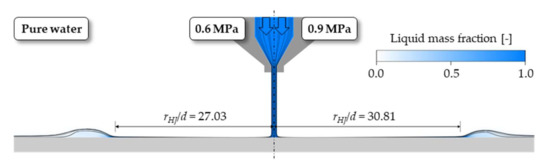
Figure 11.
Dimensionless radial position of the hydraulic jump for the cases of the inlet pressures of 0.6 (left) and 0.9 MPa (right) for pure water.
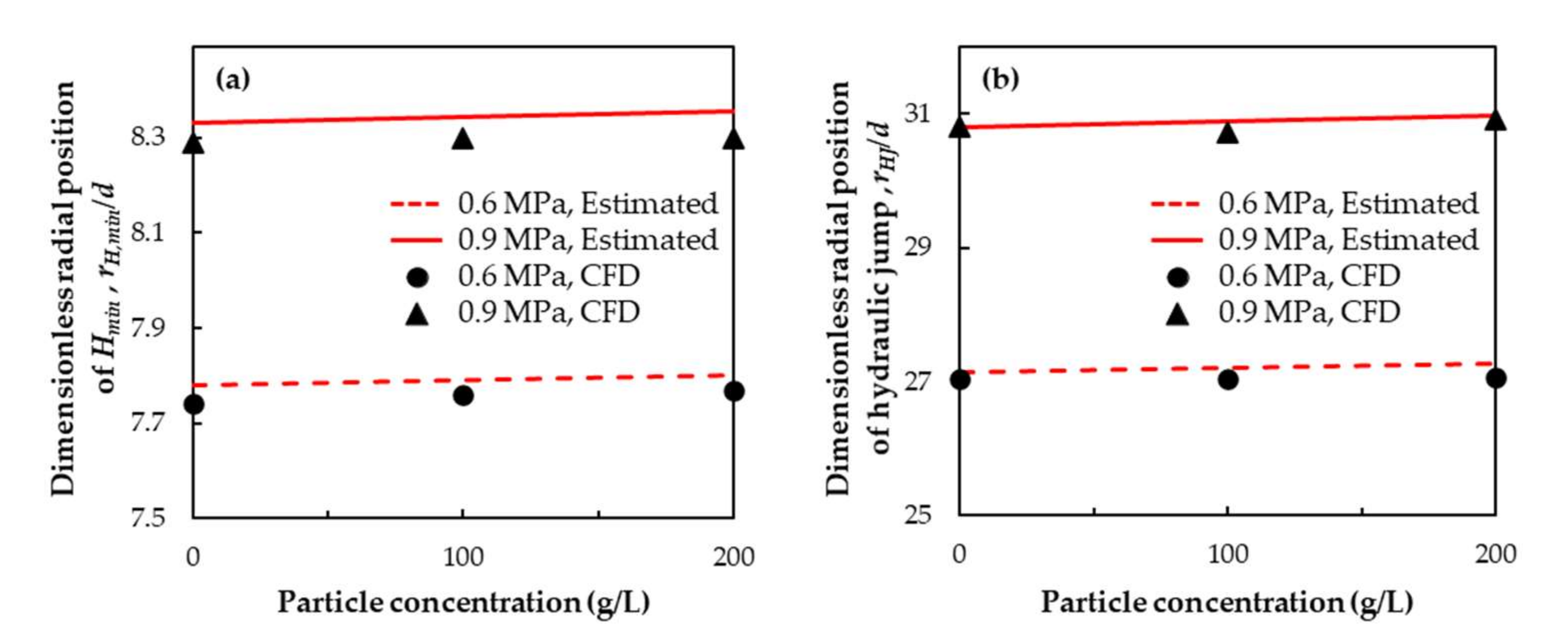
A comparison of the radial positions, where the minimum film height and the hydraulic jump occur between the results from the CFD simulations and the empirical equations, is presented in Figure 12. For the analytical estimation of these two characteristic positions, Equations (17) and (24) are used, respectively. A good agreement between these results is observed. The radial position corresponding to the minimum liquid height showed the most significant divergence, with a maximum absolute error of 0.65%, for the cases with an inlet pressure of 0.9 MPa (Figure 12a). The hydraulic jump position (Figure 12b) presented a maximum absolute error of 0.76% for the case of 0.6 MPa inlet pressure and particle concentration of 200 g/L (2.94 vol. concentration).
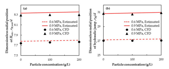
Figure 12.
Comparison of the dimensionless radial position of (a) minimum liquid film height and (b) hydraulic jump obtained from CFD simulations (symbols) and empirical formulation (lines).
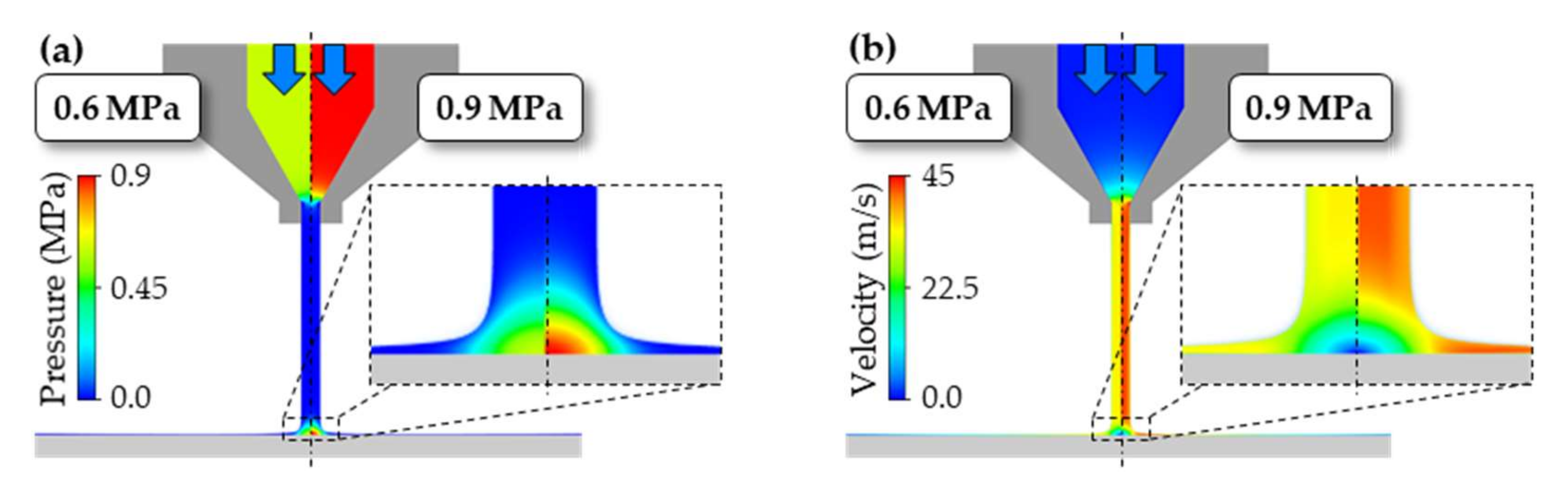
The results of the pressure and velocity fields of the impinging jet with pure water are presented in Figure 13. In the center of the liquid jet is the stagnation region (highlighted in Figure 13), where the fluid pressure, with its value being similar to the inlet pressure, has a maximum, and the fluid velocity is zero. The fluid pressure profile on the workpiece surface presents a Gaussian distribution (Figure 14a), while the tangential velocity profile has an inverted W-shape (Figure 14b).
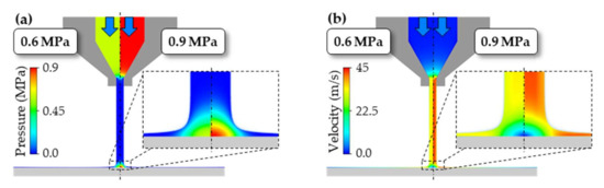
Figure 13.
Numerical results of pressure (a) and velocity (b) fields of liquid jet impinging the workpiece surface. The liquid is water with an inlet pressure of 0.6 and 0.9 MPa.

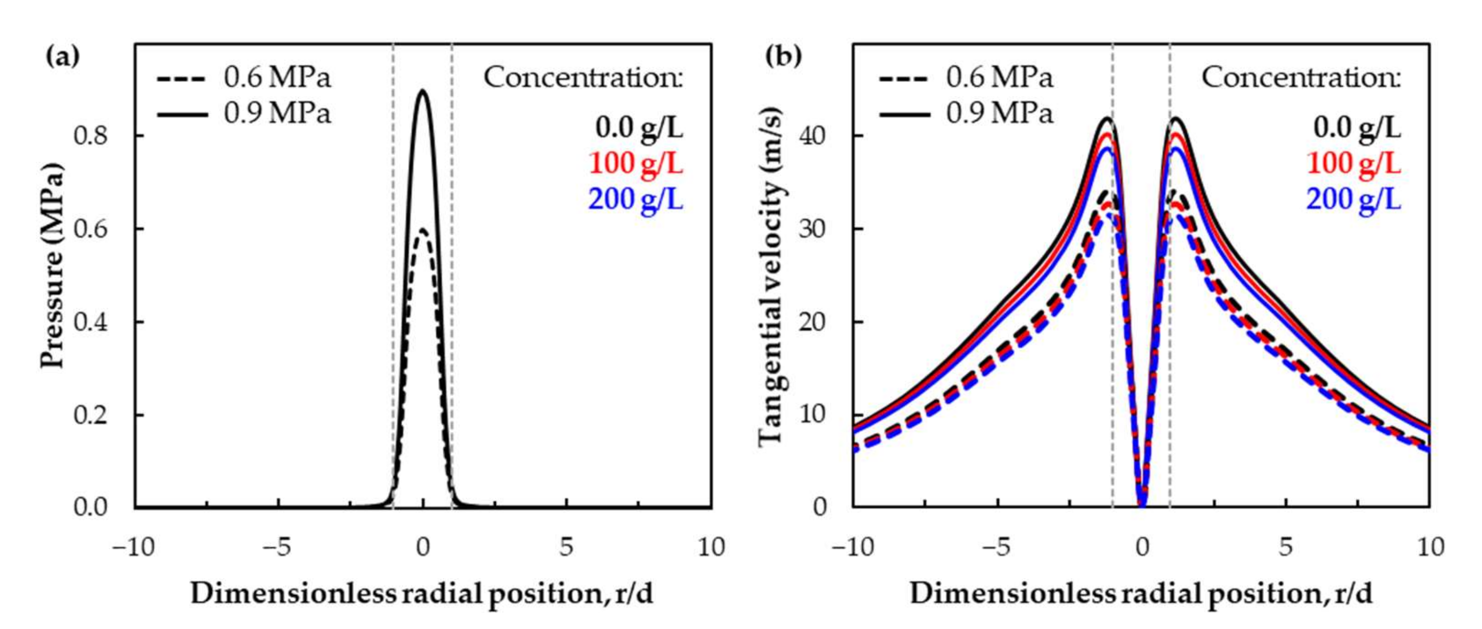
Figure 14.
Numerical results of (a) wall pressure and (b) tangential velocity profiles of the liquid fluid flow. Liquid with different particle concentrations (0.0 g/L: black lines; 100 g/L: red lines; 200 g/L: blue lines). Pressure profiles are almost identical for different particle concentrations.
The numerical results of the pressure profiles of the liquid jet on the workpiece surface present similar behavior (the curves overlap each other) when compared to the different particle concentrations in the liquid suspension, and the maximum liquid pressure on the workpiece surface is similar to the inlet pressure (Figure 14a), with values of 0.6 MPa and 0.9 MPa at the center of the jet (r/d = 0). On the other hand, slight differences are observed in the tangential velocity profiles of the liquid when different suspension concentrations are analyzed (Figure 14b). The maximum tangential velocity reduces by ~4% and ~7.6% when the particle concentration is increased from 0 to 100 g/L and from 0 to 200 g/L, respectively. As shown in Figure 14b, increasing the inlet pressure leads to a higher tangential velocity of the liquid flow.
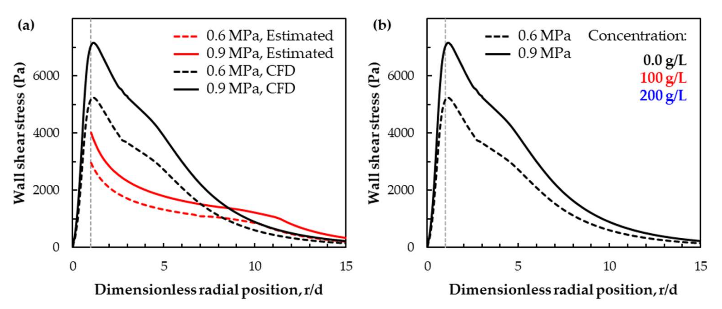
Figure 15a presents the results of wall shear stress calculated with empirical formulations and from CFD simulations. Contrary to the results of the liquid film thickness and radial positions of the minimum film thickness and hydraulic jump, the comparison between empirical approaches and numerical simulations does not present a good agreement. One explanation for the differences between the CFD results and the empirical/algebraic equation results is that the algebraic equations estimate the wall shear stress based on the Reynolds number, which is estimated for the flow conditions at the nozzle exit, while the CFD model estimates the wall shear stress based on the turbulence behavior and fluid properties in the immediate wall proximity of the workpiece surface. Therefore, the results of the flow behavior and characteristics in the region near the workpiece surface can diverge depending on which model is chosen to predict them. Similar to the pressure on the workpiece surface, the particle concentration does not affect the wall shear stress, as shown in Figure 15b. This behavior is expected since the fluid velocity decreases as the fluid viscosity and density increase, and the Reynolds number is almost constant by increasing the fluid viscosity and density (see Figure 8 and Figure 9). The wall shear stress has a value of approximately zero in the center of the impinging fluid jet. With increasing the radial position up to r/d ≈ 1, the shear stress increases significantly, reaching the maximum value.
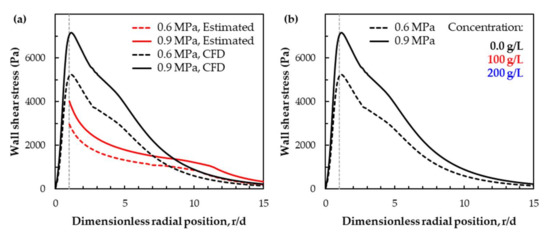
Figure 15.
Wall shear stress generated by the liquid suspension on the workpiece surface; (a) comparison between numerical results (red lines) and empirical approach (black lines); (b) comparison between different operating conditions and particle concentrations. Varying the particle concentration has no effects on the wall shear stress, and the curves overlap each other.
The radial position where the maximum wall shear stress is observed corresponds to the position where the maximum tangential liquid flow velocity is identified (Figure 14b). After that, the wall shear stress decreases, and at r/d ≈ 5, the curve profile shows a shoulder and thereafter decreases significantly up to r/d ≈ 8. This shoulder is also observed in the results from the empirical estimations but in the radial position further downstream, r/d > 10 (0.6 MPa) and r/d > 12 (0.9 MPa). Within the applied mathematical modeling, varying the particle concentration has no effects on the wall shear stress, and the curves of the shear stress profile overlap each other.
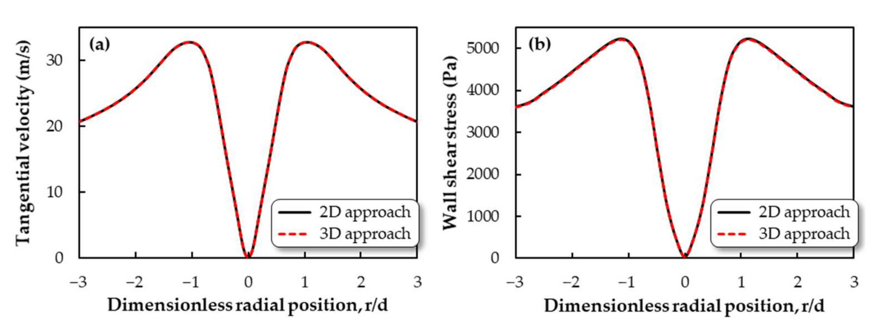
A comparison between the results from the 2D and 3D approaches of tangential velocity and wall shear stress obtained with an inlet pressure of 0.6 MPa and a particle concentration of 100 g/L is presented in Figure 16. A good agreement is observed between the 2D and 3D results, and both numerical domains present the same values. In the 3D domain, the tangential velocity and the wall shear stress are calculated with a line crossing the center of the fluid jet.
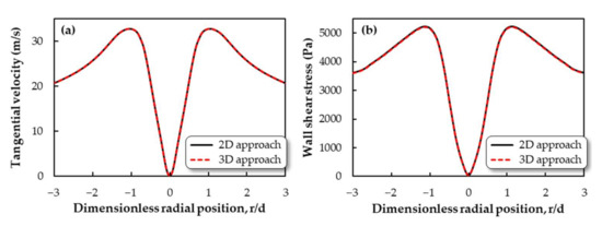
Figure 16.
Comparison of 2D (solid black lines) and 3D (dashed red lines) approaches: (a) tangential velocity and (b) wall shear stress.
4.2. Particle Hydrodynamics and Its Interaction with the Workpiece Surface
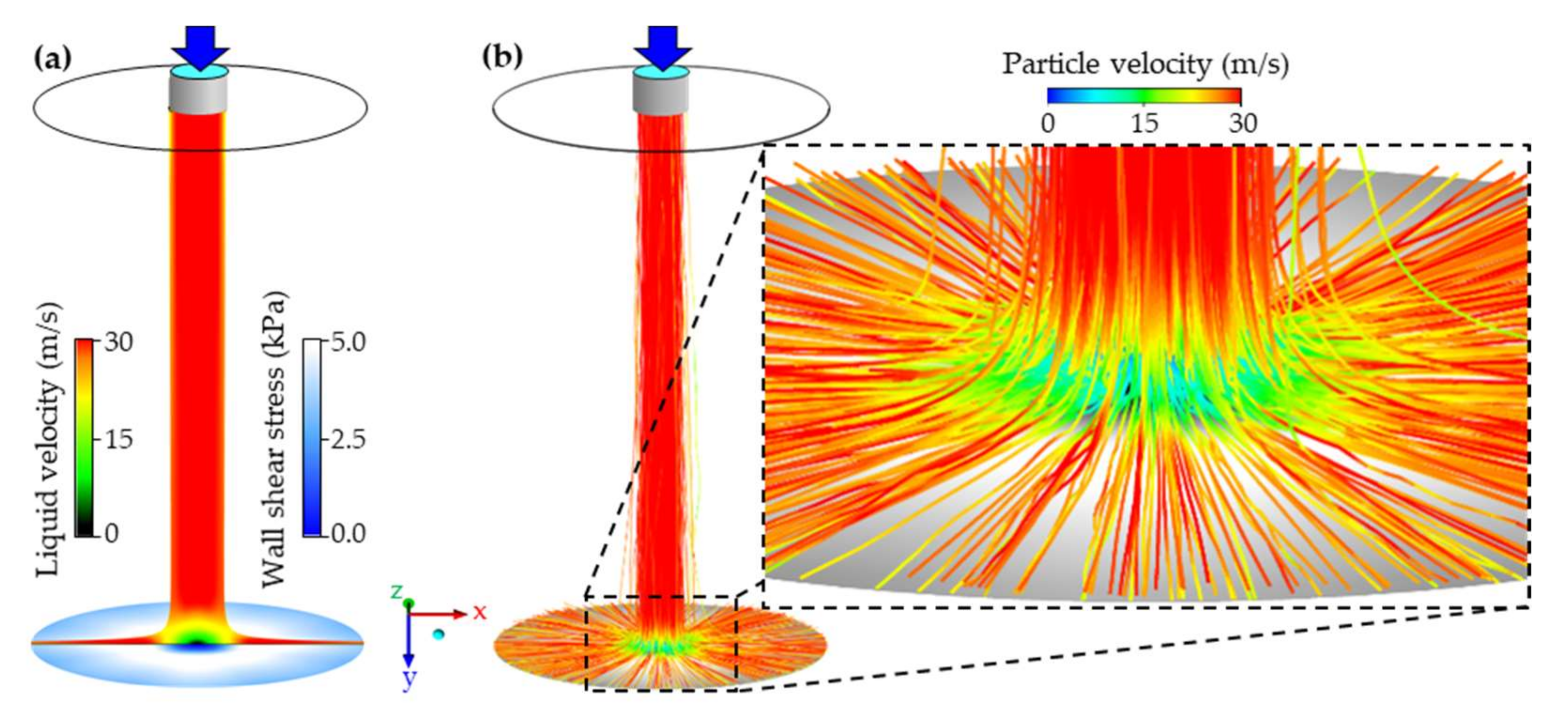
Numerical simulations of the flow with particles have been performed in a fully 3D numerical domain (Figure 4b) with an inlet pressure of 0.6 MPa and particle concentration of 100 g/L (1.47% volume concentration). The deceleration of the liquid in the stagnation region reduces the impact velocity of the particles on the workpiece surface, and, in several cases, this can produce a material removal distribution with a footprint (also called tool influence function—TIF) with a ring shape (W-shape on the sectional profile) of the workpiece surface topography. The results regarding the impact velocity of the particles and their impact angle are presented in this section.
Figure 17a presents the wall shear stress generated by the liquid suspension on the workpiece surface. The wall shear stress is almost zero in the center of the impingement zone and increases radially as the liquid velocity increases. From d ≈ 1 mm onwards, the wall shear stress increases strongly, presenting the maximum value at 1.5 mm < d < 3 mm, after which its value starts to decrease. The particle trajectories and their respective velocities are presented in Figure 17b. Due to the liquid suspension deceleration and the relatively low Stokes number of the particles, the particles are also deaccelerated near the impinging zone, reducing the velocity from ~30 m/s to ~16 m/s (averaged value).

Figure 17.
Numerical results of (a) liquid velocity field and the wall shear stress, and (b) particle trajectories and particle velocity.
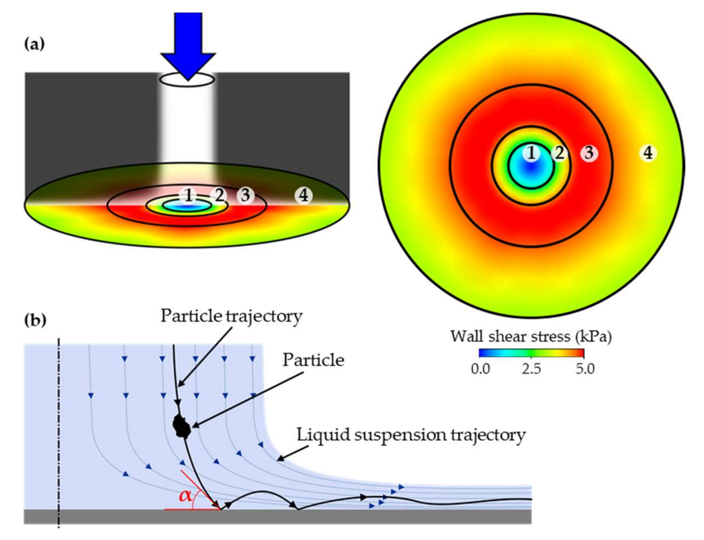
A statistical analysis of the particle trajectories and the interaction with the workpiece surface is presented in Table 4. For this analysis, the workpiece surface was divided into different regions according to the wall shear stress value, as presented in Figure 18. Region 1 is the stagnation region which has a diameter of 1.0 mm (r/d = 0.5). Region 2 is between 1.0 and 1.5 mm (0.5 < r/d < 0.75). Region 3, between 1.5 and 3 mm (0.75 < r/d < 1.5), covers the higher wall shear stress. Region 4 (r/d > 1.5) is from a diameter larger than 3.0 mm, where the shear stress starts to decrease.
Table 4.
Statistical values of the particle interaction with the workpiece surface.
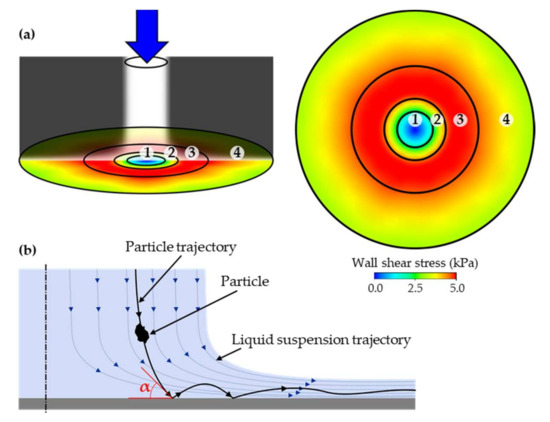
Figure 18.
(a) Division of the workpiece surface according to the wall shear stress and (b) a sketch of typical fluid and particle trajectory inside the suspension flow.
Almost half of the particles impinge the workpiece surface in the stagnation region (region 1) for the first time, with an impact angle of ~86 degrees. However, due to the deceleration of the liquid suspension flow, the particles are also decelerated. The particle velocity is reduced from ~30 m/s (free jet/exit of the nozzle) to a first impact velocity of ~15 m/s (mean velocity of the first wall touch, weighted by the particle mass flow). This represents a reduction of ~50% in the particle velocity due to the deceleration of the fluid flow. In this region, the average number of impingements per particle is 1.58, i.e., there are ~158 impingements coming from ~100 particles. In other words, particles are impinging the workpiece surface more than one time within region 1. For instance, if it is supposed that 1000 particles are injected with the suspension flow, ~502 particles are hitting the workpiece surface in region 1, and from these particles, 58% (~291 particles) are experiencing two impacts with the surface (if it is assumed that each particle hits at most twice the workpiece surface). As the material removal rate is a function of the impact velocity and angle of the particles (among other factors) [22], a low material removal rate is expected due to the low impact velocity of the particles, even though a large number of particles are impinging region 1.
Further, ~30% of particles impinge the workpiece surface for the first time within region 2, with an impact angle of ~67 degrees. The number of impingements is reduced from 1.58 (in region 1) to 1.26. The number of impingements per particle is accounted only for those particles experiencing the first touch within the analyzed region and do not consider the particles coming (and have already impinged) from region 1, for instance. The particle velocity reduction is less drastic in this region than in region 1. It is reduced from ~30 m/s to ~23 m/s, representing a deceleration of ~23.3%.
In region 3, where the highest wall shear stress is observed, the particles only decelerate from ~30 m/s to 28 m/s, representing a velocity reduction of ~6.7%. However, in this region, the number of particles impinging the workpiece surface for the first time is only 5.2% of the total particles, with an impact angle of ~26 degrees. Of course, it is expected that those particles that already impinged the workpiece surface in regions 1 and 2 also hit the surface further downstream again, and they are reaccelerated by the liquid flow, as shown in Figure 17b.
In region 4, the wall shear stress decreases considerably and the particles impinging this region for the first time are ~4% of the total particles present in the suspension. The velocity of those particles impacting the workpiece surface is ~26 m/s with an impact angle of ~7 degrees. According to the data presented in Table 4, ~90% of the total particles impinge at least once with the workpiece surface in the applied numerical domain (3D approach), i.e., ~10% of the injected particles leave the numerical domain without touching the surface.
5. Conclusions
In this study, the suspension jet impinging the workpiece surface has been investigated through numerical simulations. A systematic investigation of the fundamentals of flow behavior has been carried out to validate the mathematical model with results obtained through empirical approximations. A Eulerian–Eulerian–Lagrangian approach implemented in Ansys Fluent v.20.0 has been adopted for the flow simulations. With the applied mathematical model, it is feasible to capture the main features of the interaction of the particle suspension and the workpiece surface and to identify the impact zones, velocity, and angle of the abrasive particles on the workpiece surface. Additionally, this mathematical approach generates confident numerical results at a reasonable computational cost. Some specific conclusions are summarized:
- (1)
- A Eulerian–Eulerian approach, which treats the air and the liquid suspension as continuum phases, was applied to validate the CFD model, identifying the main flow regimes of the liquid film on the workpiece surface and evaluating their interactions.
- (2)
- A Eulerian–Eulerian–Lagrangian approach, which beyond the continuum phases also takes into account the abrasive particles as a dispersed phase, was used in the CFD simulations to calculate the particle behavior in the fluid jet polishing process and, with this, to derive a statistical analysis based on the different impinging regions of the workpiece surface.
- (3)
- This statistical analysis is essential since it allows to identify where the particles are impacting the workpiece surface and under which conditions (for instance, impact velocity and angle), allowing to design new finishing approaches and optimize the performance of the fluid jet polishing process.
- (4)
- Despite the large number of particles impinging the stagnation zone (region 1), a low material removal rate is expected due to the low impact velocity of the particles. The material removal rate is expected to be more significant in the further downstream regions, especially in which the wall shear stress increases (region 2) and presents its maxima (region 3).
- (5)
- The applied CFD approach provides a deeper understanding of the fluid suspension behavior, the particle dynamics, and the particle–wall interactions and can be applied for further investigations in order to establish correlations between the microscopic fluid–particle dynamic characteristics and the macroscopic operating process parameters.
Author Contributions
Conceptualization, L.B. and U.F.; methodology, L.B.; software, L.B. and U.F.; validation, L.B.; formal analysis, L.B., U.F. and Y.Q.; investigation, J.H., L.B. and Y.Q.; resources, O.R. and U.F; data curation, L.B.; writing—original draft preparation, L.B.; writing—review and editing, L.B. and Y.Q.; visualization, L.B.; supervision, O.R. and U.F.; project administration, O.R. and U.F.; funding acquisition, O.R. and U.F. All authors have read and agreed to the published version of the manuscript.
Funding
This research was funded by the DFG—Deutsche Forschungsgemeinschaft (German Research Foundation), project numbers FR 912/45-1 and RI 1108/12-1.
Conflicts of Interest
The authors declare no conflict of interest. The funders had no role in the design of the study, in the collection, analyses, or interpretation of data, in the writing of the manuscript, or in the decision to publish the results.
Nomenclature
| 2D | Related to a two-dimensional approach for the numerical discretization |
| 3D | Related to a three-dimensional approach for the numerical discretization |
| CFD | Computational fluid dynamics |
| DNS | Direct numerical simulations |
| DPM | Discrete phase model |
| DRW | Discrete random walk model |
| FEM | Finite element method |
| FJP | Fluid jet polishing |
| FVM | Finite-volume method |
| GCI | Grid convergence index |
| IBM | Immersed boundary method |
| LBM | Lattice–Boltzmann method |
| LES | Large-eddy simulations |
| MFJP | Microfluid jet polishing |
| PDE | Partial differential equations |
| RANS | Reynolds-averaged Navier–Stokes |
| RRSB | Rosin–Rammler–Sperling–Bennet distribution function |
| SOD | Stand-off distance |
| SST | Shear-stress transport |
| TIF | Tool influence function |
| VoF | Volume of fluid model |
| Frc | Critical Froude number |
| Fr | Froude number |
| Re | Reynolds number |
| Stokes number | |
| Dimensionless velocity gradient | |
| Nozzle diameter (m) | |
| Mean particle diameter of the RRSB distribution function (m) | |
| Sauter mean diameter (m) | |
| Particle diameter (m) | |
| Characteristic cell size (m) | |
| Liquid film thickness (m) | |
| Turbulent kinetic energy (m2 s−2) | |
| Number density of particles (# m−3) | |
| Pressure (Pa) | |
| Ambient pressure (Pa) | |
| Overpressure (Pa) | |
| Pressure in the stagnation region (Pa) | |
| Radius/radial position (m) | |
| Radial position when r = d (m) | |
| Radial position of the minimum liquid film thickness (m) | |
| Radial position where the hydraulic jump occurs (m) | |
| Radial position where the transition flow regime starts (m) | |
| Radial position where the transition flow regime ends and the fully turbulent flow starts (m) | |
| Radial position where the viscous boundary layer reaches the liquid film surface | |
| Liquid velocity at the exit of the nozzle (m s−1) | |
| Mean velocity of the fluid film (m s−1) | |
| Liquid velocity at the film surface (m s−1) | |
| Mean fluctuation velocity of particles (m s−1) | |
| Volume fraction of the liquid in the numerical element | |
| Thickness of the viscous boundary layer (m) | |
| Dissipation rate of the turbulent kinetic energy (m2 s−3) | |
| Dynamic viscosity of the pure liquid (kg m−1 s−1) | |
| Dynamic viscosity of the liquid suspension (kg m−1 s−1) | |
| Turbulent viscosity (kg m−1 s−1) | |
| Liquid suspension density (kg m−3) | |
| Liquid density (kg m−3) | |
| Particle density (kg m−3) | |
| Characteristic interparticle collision time (s) | |
| Characteristic particle relaxation time (s) | |
| Wall shear stress (Pa) | |
| Volume concentration of the solid dispersed particles in the liquid suspension | |
| Φ | Variable of the GCI method |
| Specific dissipation rate of the turbulent kinetic energy (s−1) |
References
- Schönemann, L.; Riemer, O. Thermo-mechanical tool setting mechanism for ultra-precision milling with multiple cutting edges. Precis. Eng. 2019, 55, 171–178. [Google Scholar] [CrossRef]
- Brinksmeier, E.; Mutlugünes, Y.; Klocke, F.; Aurich, J.C.; Shore, P.; Ohmori, H. Ultra-precision grinding. CIRP Ann. 2010, 59, 652–671. [Google Scholar] [CrossRef]
- Evans, C.J.; Paul, E.; Dornfeld, D.; Lucca, D.A.; Byrne, G.; Tricard, M.; Klocke, F.; Dambon, O.; Mullany, B.A. Material Removal Mechanisms in Lapping and Polishing. CIRP Ann. 2003, 52, 611–633. [Google Scholar] [CrossRef] [Green Version]
- Fähnle, O.W.; van Brug, H.; Frankena, H.J. Fluid jet polishing of optical surfaces. Appl. Opt. 1998, 37, 6771–6773. [Google Scholar] [CrossRef] [Green Version]
- Fähnle, O.W.; van Brug, H. Finishing of Optical Materials Using Fluid Jet Polishing. In Proceedings of the Annual Meeting of the American Society for Precision Engineering, Monterey, CA, USA, 31 October–5 November 1999; pp. 509–512. [Google Scholar]
- Nouraei, H.; Kowsari, K.; Papini, M.; Spelt, J.K. Operating parameters to minimize feature size in abrasive slurry jet micro-machining. Precis. Eng. 2016, 44, 109–123. [Google Scholar] [CrossRef]
- Beaucamp, A.; Namba, Y.; Freeman, R. Dynamic multiphase modeling and optimization of fluid jet polishing process. CIRP Ann. 2012, 61, 315–318. [Google Scholar] [CrossRef]
- Fähnle, O.W.; Doetz, M.; Dambon, O. Analysis of critical process parameters of ductile mode grinding of brittle materials. Adv. Opt. Technol. 2017, 6, 349–358. [Google Scholar] [CrossRef]
- Wang, C.J.; Cheung, C.F.; Ho, L.T.; Loh, Y.M. An Investigation of Effect of Stand-Off Distance on the Material Removal Characteristics and Surface Generation in Fluid Jet Polishing. Nanomanuf. Metrol. 2020, 3, 112–122. [Google Scholar] [CrossRef]
- Beaucamp, A.; Freeman, R.; Matsumoto, A.; Namba, Y. Fluid jet and bonnet polishing of optical moulds for application from visible to X-ray. In Proceedings of the SPIE 8126—Optical Engineering and Applications, San Diego, CA, USA, 27 September 2011. [Google Scholar]
- Booij, S.M.; van Brug, H.; Braat, J.J.M.; Fähnle, O.W. Nanometer deep shaping with fluid jet polishing. Opt. Eng. 2002, 41, 1926–1931. [Google Scholar] [CrossRef]
- Booij, S.M.; Fähnle, O.W.; Meeder, M.; Wons, T.; Braat, J.J.M. Jules Verne: A new polishing technique related to FJP. In Proceedings of the SPIE, San Diego, CA, USA, 22 December 2003; SPIE: Bellingham, WA, USA, 2003; Volume 5180, pp. 89–100. [Google Scholar]
- Messelink, W.A.C.M.; Fähnle, O.W. Exploiting the Process Stability of Fluid Jet Polishing. In Proceedings of the Frontiers in Optics 2008/Laser Science XXIV/Plasmonics and Metamaterials/Optical Fabrication and Testing, Rochester, NY, USA, 21–24 October 2008; p. OThD3. [Google Scholar]
- Fähnle, O. Process optimization in optical fabrication. Opt. Eng. 2016, 55, 035106. [Google Scholar] [CrossRef]
- Beaucamp, A.; Namba, Y. Super-smooth finishing of diamond turned hard X-ray molding dies by combined fluid jet and bonnet polishing. CIRP Ann. 2013, 62, 315–318. [Google Scholar] [CrossRef]
- Beaucamp, A.; Katsuura, T.; Kawara, Z. A novel ultrasonic cavitation assisted fluid jet polishing system. CIRP Ann. 2017, 66, 301–304. [Google Scholar] [CrossRef]
- Chaves-Jacob, J.; Beaucamp, A.; Zhu, W.; Kono, D.; Linares, J.-M. Towards an understanding of surface finishing with compliant tools using a fast and accurate simulation method. Int. J. Mach. Tool Manu. 2021, 163, 103704. [Google Scholar] [CrossRef]
- Wang, C.J.; Cheung, C.F.; Ho, L.T.; Liu, M.Y.; Lee, W.B. A novel multi-jet polishing process and tool for high-efficiency polishing. Int. J. Mach. Tools Manuf. 2017, 115, 60–73. [Google Scholar] [CrossRef]
- Li, Z.; Li, S.; Dai, Y.; Peng, X. Optimization and application of influence function in abrasive jet polishing. Appl. Opt. 2010, 49, 2947–2953. [Google Scholar] [CrossRef]
- Li, Z.; Wang, J.M.; Peng, X.Q.; Ho, L.T.; Yin, Z.Q.; Li, S.Y.; Cheung, C.F. Removal of single point diamond-turning marks by abrasive jet polishing. Appl. Opt. 2011, 50, 2458–2463. [Google Scholar] [CrossRef] [Green Version]
- Matsumura, T.; Muramatsu, T.; Fueki, S. Abrasive water jet machining of glass with stagnation effect. CIRP Ann. 2011, 60, 355–358. [Google Scholar] [CrossRef]
- Cao, Z.-C.; Cheung, C.F. Theoretical modelling and analysis of the material removal characteristics in fluid jet polishing. Int. J. Mech. Sci. 2014, 89, 158–166. [Google Scholar] [CrossRef]
- Cao, Z.-C.; Cheung, C.F.; Zhao, X. A theoretical and experimental investigation of material removal characteristics and surface generation in bonnet polishing. Wear 2016, 360–361, 137–146. [Google Scholar] [CrossRef]
- Fritsching, U. Spray Simulation—Modeling and Numerical Simulation of Sprayforming Metals; Cambridge University Press: Cambridge, UK, 2004. [Google Scholar]
- Mousazadeh, S.M.; Shahmardan, M.M.; Tavangar, T.; Hosseinzadeh, K.; Ganji, D.D. Numerical investigation on convective heat transfer over two heated wall-mounted cubes in tandem and staggered arrangement. Theor. Appl. Mech. Lett. 2018, 8, 171–183. [Google Scholar] [CrossRef]
- Buss, L.; Meierhofer, F.; Bianchi Neto, P.; Meier, H.F.; Fritsching, U.; Noriler, D. Impact of co-flow on the spray flame behaviour applied to nanoparticle synthesis. Can. J. Chem. Eng. 2019, 97, 604–615. [Google Scholar] [CrossRef]
- Buss, L.; Noriler, D.; Fritsching, U. Impact of Reaction Chamber Geometry on the Particle-Residence-Time in Flame Spray Process. Flow Turbul. Combust. 2020, 105, 1055–1086. [Google Scholar] [CrossRef]
- Hosseinzadeh, K.; Ganji, D.D.; Ommi, F. Effect of SiO2 super-hydrophobic coating and self-rewetting fluid on two phase closed thermosyphon heat transfer characteristics: An experimental and numerical study. J. Mol. Liq. 2020, 315, 113748. [Google Scholar] [CrossRef]
- Bianchi Neto, P.; Buss, L.; Fritsching, U.; Noriler, D. Modelling polydisperse nanoparticle production in an enclosed flame spray pyrolysis reactor. In Proceedings of the 15th Triennial International Conference on Liquid Atomization and Spray Systems—ICLASS 2021, Edinburgh, UK, 29 October–2 September 2021. [Google Scholar]
- Hosseinzadeh, K.; Montazer, E.; Shafii, M.B.; Ganji, A.R.D. Solidification enhancement in triplex thermal energy storage system via triplets fins configuration and hybrid nanoparticles. J. Energy Storage 2021, 34, 102177. [Google Scholar] [CrossRef]
- Mardani, M.R.; Ganji, D.D.; Hosseinzadeh, K. Numerical investigation of droplet coalescence of saltwater in the crude oil by external electric field. J. Mol. Liq. 2022, 346, 117111. [Google Scholar] [CrossRef]
- Nguyen, V.B.; Nguyen, Q.B.; Liu, Z.G.; Wan, S.; Lim, C.Y.H.; Zhang, Y.W. A combined numerical–experimental study on the effect of surface evolution on the water–sand multiphase flow characteristics and the material erosion behavior. Wear 2014, 319, 96–109. [Google Scholar] [CrossRef]
- Qi, H.; Wen, D.; Lu, C.; Li, G. Numerical and experimental study on ultrasonic vibration-assisted micro-channelling of glasses using an abrasive slurry jet. Int. J. Mech. Sci. 2016, 110, 94–107. [Google Scholar] [CrossRef]
- Qi, H.; Wen, D.; Yuan, Q.; Zhang, L.; Chen, Z. Numerical investigation on particle impact erosion in ultrasonic-assisted abrasive slurry jet micro-machining of glasses. Powder Technol. 2017, 314, 627–634. [Google Scholar] [CrossRef]
- Liu, X.; Lienhard, J.H.; Lombara, J.S. Convective Heat Transfer by Impingement of Circular Liquid Jets. J. Heat Transf. 1991, 113, 571–582. [Google Scholar] [CrossRef]
- Bhagat, R.K.; Wilson, D.I. Flow in the thin film created by a coherent turbulent water jet impinging on a vertical wall. Chem. Eng. Sci. 2016, 152, 606–623. [Google Scholar] [CrossRef] [Green Version]
- Lienhard, J.H. Heat Transfer by Impingement of Circular Free-Surface Liquid Jets. In Proceedings of the 18th National & 7th ISHMT-ASME Heat and Mass Transfer Conference, Guwahati, India, 27–30 December 2006. [Google Scholar]
- Liu, X.; Gabour, L.A.; Lienhard, J.H. Stagnation-Point Heat Transfer During Impingement of Laminar Liquid Jets: Analysis Including Surface Tension. J. Heat Transf. 1993, 115, 99–105. [Google Scholar] [CrossRef] [Green Version]
- Ma, C.F.; Zhao, Y.H.; Masuoka, T.; Gomi, T. Analytical study on impingement heat transfer with single-phase free-surface circular liquid jets. J. Therm. Sci. 1996, 5, 271–277. [Google Scholar] [CrossRef]
- Martin, H. Heat and Mass Transfer between Impinging Gas Jets and Solid Surfaces. In Advances in Heat Transfer; Hartnett, J.P., Irvine, T.F., Eds.; Elsevier: Amsterdam, The Netherlands, 1977; Volume 13, pp. 1–60. [Google Scholar]
- Watson, E.J. The radial spread of a liquid jet over a horizontal plane. J. Fluid Mech. 1964, 20, 481–499. [Google Scholar] [CrossRef]
- Schlichting, H.; Gersten, K. Grenzschicht-Theorie; Springer: Berlin, Germany, 2006. [Google Scholar]
- Azuma, T.; Hoshino, T. The Radial Flow of a Thin Liquid Film: 4th Report, Stability of Liquid Film and Wall Pressure Fluctuation. Bull. JSME 1984, 27, 2763–2770. [Google Scholar] [CrossRef]
- Baonga, J.B.; Louahlia-Gualous, H.; Imbert, M. Experimental study of the hydrodynamic and heat transfer of free liquid jet impinging a flat circular heated disk. Appl. Therm. Eng. 2006, 26, 1125–1138. [Google Scholar] [CrossRef]
- ANSYS Inc. ANSYS Fluent Theory Guide; ANSYS, Inc.: Canonsburg, PA, USA, 2020. [Google Scholar]
- Menter, F.R. Two-equation eddy-viscosity turbulence models for engineering applications. AIAA J. 1994, 32, 1598–1605. [Google Scholar] [CrossRef] [Green Version]
- Annoni, M.; Arleo, F.; Malmassari, C. CFD aided design and experimental validation of an innovative Air Assisted Pure Water Jet cutting system. J. Mater. Process. Technol. 2014, 214, 1647–1657. [Google Scholar] [CrossRef] [Green Version]
- Crowe, C.T.; Schwarzkopf, J.D.; Sommerfeld, M.; Tsuji, Y. Multiphase Flows with Droplets and Particles; CRC Press: Boca Raton, FL, USA, 2011. [Google Scholar]
- Gosman, A.D.; Ioannides, E. Aspects of Computer Simulation of Liquid-Fueled Combustors. J. Energy 1983, 7, 482–490. [Google Scholar] [CrossRef]
- Morsi, S.A.; Alexander, A.J. An investigation of particle trajectories in two-phase flow systems. J. Fluid Mech. 1972, 55, 193–208. [Google Scholar] [CrossRef]
- Rosin, P.; Rammler, E. The laws governing the fineness of powdered coal. J. Inst. Fuel 1933, 7, 29–36. [Google Scholar]
- Mugele, R.A.; Evans, H.D. Droplet Size Distribution in Sprays. Ind. Eng. Chem. 1951, 43, 1317–1324. [Google Scholar] [CrossRef]
- Alderliesten, M. Mean Particle Diameters. Part VII. The Rosin-Rammler Size Distribution: Physical and Mathematical Properties and Relationships to Moment-Ratio Defined Mean Particle Diameters. Part. Part. Syst. Charact. 2013, 30, 244–257. [Google Scholar] [CrossRef]
- Celik, I.B.; Ghia, U.; Roache, P.J.; Freitas, C.J.; Coleman, H.; Raad, P.E. Procedure for Estimation and Reporting of Uncertainty Due to Discretization in CFD Applications. J. Fluid Eng. 2008, 130, 078001. [Google Scholar] [CrossRef] [Green Version]
- Breki, A.; Nosonovsky, M. Einstein’s Viscosity Equation for Nanolubricated Friction. Langmuir 2018, 34, 12968–12973. [Google Scholar] [CrossRef]
- Einstein, A. Eine neue Bestimmung der Moleküldimensionen. Ann. Phys. 1906, 324, 289–306. [Google Scholar] [CrossRef] [Green Version]
- Einstein, A. Berichtigung zu meiner Arbeit: “Eine neue Bestimmung der Moleküldimensionen”. Ann. Phys. 1911, 339, 591–592. [Google Scholar] [CrossRef] [Green Version]


Publisher’s Note: MDPI stays neutral with regard to jurisdictional claims in published maps and institutional affiliations. |
© 2022 by the authors. Licensee MDPI, Basel, Switzerland. This article is an open access article distributed under the terms and conditions of the Creative Commons Attribution (CC BY) license (https://creativecommons.org/licenses/by/4.0/).