Article

Calibration of the k-ω SST Turbulence Model for Free Surface Flows on Mountain Slopes Using an Experiment

1
Ivannikov Institute for System Programming, Russian Academy of Sciences, Alexander Solzhenitsyn St., 25, 109004 Moscow, Russia
2
Faculty of Mechanics and Mathematics, Lomonosov Moscow State University, GSP-1, 1 Leninskiye Gory, 119991 Moscow, Russia
3
Research Institute of Mechanics, Lomonosov Moscow State University, 1 Michurinsky Pr., 119192 Moscow, Russia
4
Faculty of Geography, Lomonosov Moscow State University, GSP-1, 1 Leninskiye Gory, 119991 Moscow, Russia
5
Faculty of Physics, Lomonosov Moscow State University, GSP-1, 1-2 Leninskiye Gory, 119991 Moscow, Russia
*
Author to whom correspondence should be addressed.
Fluids 2022, 7(3), 111; https://doi.org/10.3390/fluids7030111
Submission received: 18 February 2022 / Revised: 11 March 2022 / Accepted: 15 March 2022 / Published: 17 March 2022

Abstract

:
We calibrate the k- ω S S T turbulence model for free surface flows in the channel or on the slope using machine learning techniques. To calibrate the turbulence model, an experiment is carried out in an inclined rectangular research chute. In the experiment, the pressure values in the flow are measured at different distances from the bottom; after transforming data, the flow velocity profile is obtained. The k- ω S S T turbulence model is calibrated based on experimental data using the Nelder-Mead optimization algorithm. The calibrated turbulence model is then used to calculate the glacial lake Maliy Azau outburst flood on the Elbrus (Central Caucasus).

1. Introduction

This article is part of the authors’ work on the creation of three-dimensional mathematical and numerical models of various geophysical flows on mountain slopes. Snow avalanches, mudflows, catastrophic torrents, landslides, lava flows, etc. are examples of such flows. These flows can pose a great danger to the life and activities of people in the mountains. To organize protection against them, information is needed about the boundaries of propagation of such flows, as well as about their sizes and speeds. One way to obtain this information is through mathematical modeling.
Geophysical flows on the slopes are very diverse in scales, properties of the moving medium and the type of motion (laminar or turbulent). The materials that form the flow usually have complex non-Newtonian rheological properties (non-linear viscosity, yield stress, etc.). Descent of a slope flow can be accompanied by mixing with the ambient air, as well as entrainment of the underlying material, which significantly affects the flow dynamics and leads to erosion of slopes. It is clear that for flows of different types, it is necessary to create and use different mathematical models.
Depending on the degree of detail in the description of the flow parameters, mathematical models can be divided into three classes: (1) models in which the entire flow is presented as the movement of a material point down the slope; (2) models based on equations averaged over the flow depth, similar to the shallow water equations used in hydraulics; these models are one-dimensional or two-dimensional because the depth-averaged flow parameters depend on one or two coordinates along the slope surface; (3) three-dimensional models based on complete (not averaged over depth) equations, including the dependence of the flow parameters along the normal to the bottom. Up to date models based on equations averaged over the flow depth are mainly used, these are such works as [1,2,3,4,5,6,7], dating from 1967. Further development of depth-averaged models was the use of the two-dimensional approach [8,9,10,11]. Currently, the use of depth-averaged equations can be seen in the works [12,13,14,15,16,17,18]. A detailed review can be found in [5]. However, to calculate the forces acting when a flow hits an obstacle, in particular, a protective structure or a building located in its path, it is necessary to know not only the depth-average values of the flow parameters, but also their distribution along the depth. In this regard, three-dimensional models are developing. First 3D powder-snow avalanches models were developed in the early 1990s [19,20,21]. At the moment, three-dimensional models are developing especially actively. This is facilitated by the emergence of new computational methods, as well as the development and widespread use of computing technology.
There are several articles in the literature devoted to 3D models of slope currents [22,23,24,25]. Basically, 3D models are used to simulate flows, the density of which is comparable to the density of the surrounding air, namely, powder snow avalanches [26,27,28]. In this case, the most important factor is mixing with the air (or with the surrounding water if these are underwater turbidity currents). Three-dimensional models of dense snow avalanches are described in [22,23]. These articles assume that the movement is laminar and there is no mixing with the ambient air.
The subject of our paper is 3D modeling of turbulent slope flows. We use the Reynolds-averaged approach including semi-empirical models to describe turbulence. We suppose that the k- ω   S S T turbulence model can be applied to describe free-surface turbulent slope flows when model coefficients were calibrated properly. Calibration of k- ω   S S T [29,30,31] models was mainly carried out for such cases as airflow around various profiles. Calibration was also carried out for the flow around simple flat plate [32] and small-sized wind turbines [33,34]. So there was no constants calibration for free surface slope flows with splashes. In this study we develop the calibration procedure and calibrate the coefficients for water slope flows.
The structure of the paper is the following. Section 2 describes the experiments conducted at the University of Iceland (UI) and some results of our simulations by the model with standard coefficient values. In Section 3 the experimental device is shortly described which was built at the Institute of Mechanics Lomonosov Moscow state university (MSU) and was used to calibrate the k- ω   S S T model. The mathematical model, the software and the optimization algorithm are described in Section 4, Section 5 and Section 6. Calibrated coefficients values and results of simulations of the flows in the experimental chutes of MSU and UI with calibrated coefficients are presented in Section 7 and Section 8. In Section 9 the results of a simulation of a glacial lake outburst flood (GLOF) at the glacier Maliy Azau (Mt. elbrus, Caucasus) are shown.

2. Relevance

The paper is devoted to turbulent slope flows in mountains, such as mudflows, slushflows, powder snow avalanches, glacial lake outburst floods, and others. Three slope flows were used for the study:
  • a turbulent water flow in an inclined experimental chute flow to calibrate the turbulence model. The experiments were conducted by the authors at the Research Institute of Mechanics of Lomonosov Moscow State University (MSU);
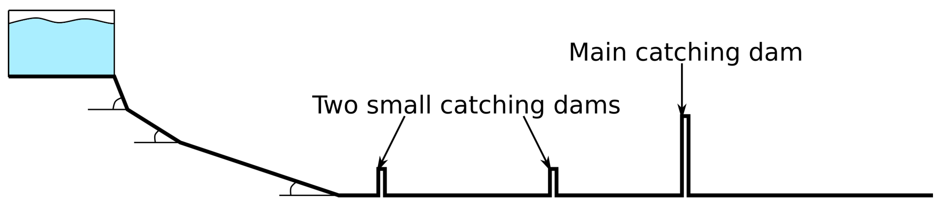
  • an experiment carried out at the University of Iceland (UI) to verify the calibration results;
  • a potential glacial lake outburst flow (GLOF) at the Maliy Azau glacier as an example of application of the model to natural geophysical mass flow.
The key parameters of the studied flows are given in Table 1. It shows that the Reynolds numbers are large enough for all studied flows to be considered turbulent.
Existing turbulence models contain a number of constants that have been calibrated for canonical flows such as air flow around various profiles, flows in pipes and channels, etc. [35,36,37]. Calibration of turbulence model coefficients for simulation flows of a different media with a free surface on mountain slopes has not been performed. To demonstrate the differences between the experimental data and the calculated ones, simulations of an experiment at the University of Iceland [38,39] were made.
The UI experiments modeled the interaction of high-speed water flows in steep terrain with protective structures, in particular, with a system of several catching dams. A scheme of the chute with two small catching dams and one main catching dam is shown in Figure 1. Tap water was used in the experiment to identify the difference between granular, high Froude number compressible flows and incompressible dense, supercritical flows. The Froude numbers were in the range of 3 < Fr < 5. The experiments were conducted on a long wooden chute that consisted of four sections with different slope angles (55 , 27 , 11.7 , 0 —from left to right). The lower 5.05 m of the chute were horizontal and the upper parts of it were carpeted to increase friction and decrease the flow speed and thus the Froude number to obtain the targeted range of Froude numbers. Catching dams were made of plywood. The main (highest) dam was placed at the lower end of the horizontal part of the chute as shown in Figure 1.
The simulations of the UI experiments were carried out using a multiphase single-velocity approach implemented in the OpenFOAM package in the interFoam solver. The calculation domain of the UI experiment at the initial moment of time is shown in Figure 2. Two most popular turbulence models, k- ε and k- ω   S S T , with standard sets of coefficients were used. Some results for a flow in the chute without barriers are shown at Figure 3. Some results for the flow in the chute with three dams are presented in the Table 2.
In this particular case—the flow without barriers—the k- ε model seems to fit the experimental results better than the k- ω   S S T model. However, in general, k- ω   S S T model has a number of advantages including the possibility to study the flow behavior both near and far from the bottom which is important for natural slope flows. The k- ω   S S T turbulence model has a wider range of applicability, since it includes switching during the calculation in an automatic mode between k- ε and k- ω turbulence models depending on the flow type—flow with high and low Reynolds numbers, respectively. That is why we decided to focus on k- ω   S S T model and try to calibrate this model coefficients.

3. Experiment for Turbulence Model Calibration

To calibrate the k- ω   S S T turbulence model coefficients, we used an experiment set up at the Research Institute of Mechanics of Lomonosov Moscow State University. The UI experiment data will be used for verification of the results. In the experiment, a turbulent fluid flow descended along a chute with a constant slope angle; the experiment was carried out for several different slope angles. The chute had the following geometry: length is 1 m, width is 12 cm, height of sides is 10 cm. The computational domain was located between two sections of velocity and depth measurements, located at distances 23 cm and 82 cm from the top edge. The scheme of the experiment is shown in Figure 4. Tap water was used for the experiment, similar to the experiment at the University of Iceland. The chute is made entirely of 4 mm acrylic glass. Water comes from a reservoir with the provided possibility of adjusting the height of the liquid column. The experiment was carried out in a stationary mode with a closed fluid circuit. Stationarity was provided by pumping water from the lower reservoir to the upper one.
Three series of experiments were carried out, in which the slope angle, the initial flow depth, the initial flow profile were different, as shown in the Table 3.

4. Mathematical Model

The flow is considered as an incompressible multiphase flow of air and water, both phases have the same speed. The k- ω   S S T turbulence model is used, based on the papers of Menter et al. [29,30,31].
We use the VOF (Volume of Fluid) method to find the shape of the free surface. This method allows to model free surface flows as well as multi-phase flows. In the present study, one phase is water and the other is air. So the water/air interface is a free surface. The computation is performed on a fixed grid, which extends beyond the free surface. The transport equation for the liquid volume concentration is solved, so the threshold value for the liquid volume fraction determines the free surface. This method has a number of advantages that are important for the problem, such as high robustness, which is very important for large-scale slope flows, when the computational mesh is unstructured and can reach many millions of cells, and the computation time is also long. Conservation of mass and momentum in the system is achieved using the VOF method, which is very important when applied to such flows on mountain slopes as, e.g., snow avalanches (which were also investigated by this method in [24,25,40]), when the mass of the flow determines the zone of the avalanche deposits.
The system of equations for describing a two-phase flow model, in which both phases are incompressible and have the same velocity (1) consists of: the continuity equation for a mixture, the volume phase fraction transport equation, the momentum conservation equation, the turbulent kinetic energy equation, and specific turbulent kinetic energy dissipation equation.
· u ¯ = 0 , α t + · ( u ¯ α ) = 0 , ( ρ u ¯ ) t + · ( ρ u ¯ u ¯ ) = p ¯ + · τ ¯ + ρ f ¯ , ( ρ k ) t + · ( ρ u ¯ k ) = P ˜ k β * ρ k ω + · ( μ + α k μ t ) k , ( ρ ω ) t + · ( ρ u ¯ ω ) = γ ρ s ˙ 2 β ρ ω 2 + · ( μ + α ω μ t ) ω + 2 ( 1 F 1 ) ρ α ω 2 1 ω k · ω .
Here u ¯ is the speed of the mixture; α —the volume fraction of the selected phase—water in this study; τ ¯ = 2 μ e f f s ¯ —the stress tensor, which is a function of the strain rate tensor s ¯ = u ¯ + ( u ¯ ) T / 2 ; μ e f f = μ + μ t —the effective viscosity, which is the sum of molecular and turbulent viscosity, μ t = ρ a 1 k / max ( a 1 ω , b 1 s ˙ F 2 ) ; a 1 and b 1 —the turbulence model constants; ρ —the mixture density; p ¯ —the pressure; f ¯ —the density of body forces; k—the turbulent kinetic energy; ω —specific turbulent kinetic energy dissipation rate; P ˜ k —production rate of turbulent kinetic energy by the Reynolds-averaged flow; F 1 —the blending function; turbulent model coefficients α k , α ω , β , γ are calculated according to the principle of the weighted average: γ = γ 1 F 1 + γ 2 ( 1 F 1 ) .
The following closing relations are used
F 1 = tanh min max k β * ω y , 500 ν y 2 ω , 4 ρ α ω 2 k C D k ω y 2 4 .
C D k ω = max 2 ρ α ω 2 1 ω k · ω , 10 10 ; y is the distance to the nearest wall ( F 1 equals zero away from the wall and model turns into the k- ε model, and switches to 1 inside the boundary layer, realizing the k- ω model); s ˙ —the invariant measure of the strain rate strain rate s ¯ ; F 2 —second blending function
F 2 = tanh max 2 k β * ω y , 500 ν y 2 ω 2 .
Also, the limiter on the growth of turbulence is used in stagnation modes
P ˜ k = min ( P k , 10 · β * ρ k ω ) , P k = μ t u ¯ · u ¯ + ( u ¯ ) T .
The following rheological model is implemented. Two incompressible and immiscible phases are represented in the computational domain by a certain mixture with physical characteristics calculated according to the principle of the weighted average (5) and (6):
ρ = ρ 1 α + ρ 0 ( 1 α ) ,
μ = ν ρ , ν = ν 1 α + ν 0 ( 1 α ) .
ρ 0 and ν 0 , ρ 1 and ν 1 are the density and effective kinematic viscosity of each phase, respectively.

5. Software

The free open source software OpenFOAM is used, which has the following advantages:
  • preprocessing utilities (mesh generation and convertation, setting specific initial and boundary conditions),
  • big base of standard solvers, a lot of extended solvers,
  • postprocessing utilities (calculation, visualisation, convertation)
  • well documented,
  • modular code,
  • the possibility of implementing new models,
  • wide distribution, many developers and users.

5.1. Numerical Method

In this study, we use the interFoam solver, which is part of the OpenFOAM package. The InterFoam solver allows you to model free surface flows as well as multiphase flows using the VOF (Volume Of Fluid) interface capturing method. In this method, an indicator function is introduced, which shows the volume fractions of different phases in the cell. The main advantage of this method is its applicability to the boundary self-crossing modeling, which makes it possible to simulate splashes [41], separation of individual drops [42], bubbles in a liquid [43], etc. Such phenomena can occur at the interaction of rapid flows with obstacles. The VOF method was proposed by Hirt and Nicholson in 1981 [44]. Later different improvements of it have been proposed. They are implemented in modern version OpenFOAM. In particular, a high-resolution compression difference scheme to approximate the terms of the transport equation for the phase volume fraction [45] is used, an improved solution algorithm [43] based on the PISO algorithm is included, a compression convective term is added to the transport equations for increasing the sharpness of the interface [42]. The VOF method with all the above improvements is used here.
The following approximation schemes are used:
  • time derivatives t : first order, bounded, implicit Euler scheme;
  • water volume fraction flux · ( u ¯ α ) : Gaussian finite volume integration with vanLeer interpolation;
  • convection term · ( ρ u ¯ u ¯ ) : Gaussian finite volume integration with upwind interpolation;
  • divergence of the stress tensor · τ ¯ : Gaussian finite volume integration with upwind interpolation;
  • turbulent kinetic energy flux · ( ρ u ¯ k ) : Gaussian finite volume integration with linear (central differencing) interpolation;
  • dissipation flux of the specific turbulent kinetic energy · ( ρ u ¯ ω ) : Gaussian finite volume integration with linear (central differencing) interpolation;
  • gradient terms : Gaussian integration with linear interpolation;
  • Laplacian terms 2 : Gaussian integration with linear interpolation with explicit non-orthogonal correction;
  • Other terms not listed above are discretized using a central difference scheme.
To solve a system of equations, the PIMPLE algorithm [46,47] is used, which is a combination of the PISO (Pressure Implicit with Splitting of Operator) and SIMPLE (Semi-Implicit Method for Pressure-Linked Equations) algorithms.

5.2. Computational Mesh for Lomonosov MSU Experiment

In the MSU experiment, the flow was simulated in the region between two sections of the trough in which measurements were made. The velocity profile and depth measured in the inlet section were used as boundary conditions; the parameters in the outlet section were calculated and compared with the measured values. The calculation was carried out for the 10 mm wide middle strip of the chute, where the influence of the side walls is insignificant. The geometry of the computational domain is a parallelepiped 590 mm long, 10 mm wide, and 60 mm deep. The number of cells was 590 × 10 × 60 .
The following boundaries of the computational domain were determined: the chute bottom (bottom of the computational domain), computational domain sides, computational domain upper border, the chute inlet, and outlet sections.
The following boundary conditions were set:
  • The chute bottom is a solid wall with the no-slip condition;
  • computational domain sides: the zero gradient condition is set to exclude the influence of sides on the flow;
  • computational domain upper border: a mixed condition with atmospheric pressure, no inflow through the border and outflow according to zero gradient condition;
  • the inlet section: fixed values of water volume fraction and flow velocity profile;
  • the outlet section: a zero gradient condition for all parameters.
The initial conditions in the problem are as follows: the domain is completely filled with stationary air, the liquid flows in through the inlet section. After some time, the flow becomes steady and measurements are taken in the outlet section, which are compared with the experimental data. The flow is considered to be steady after 5 s.

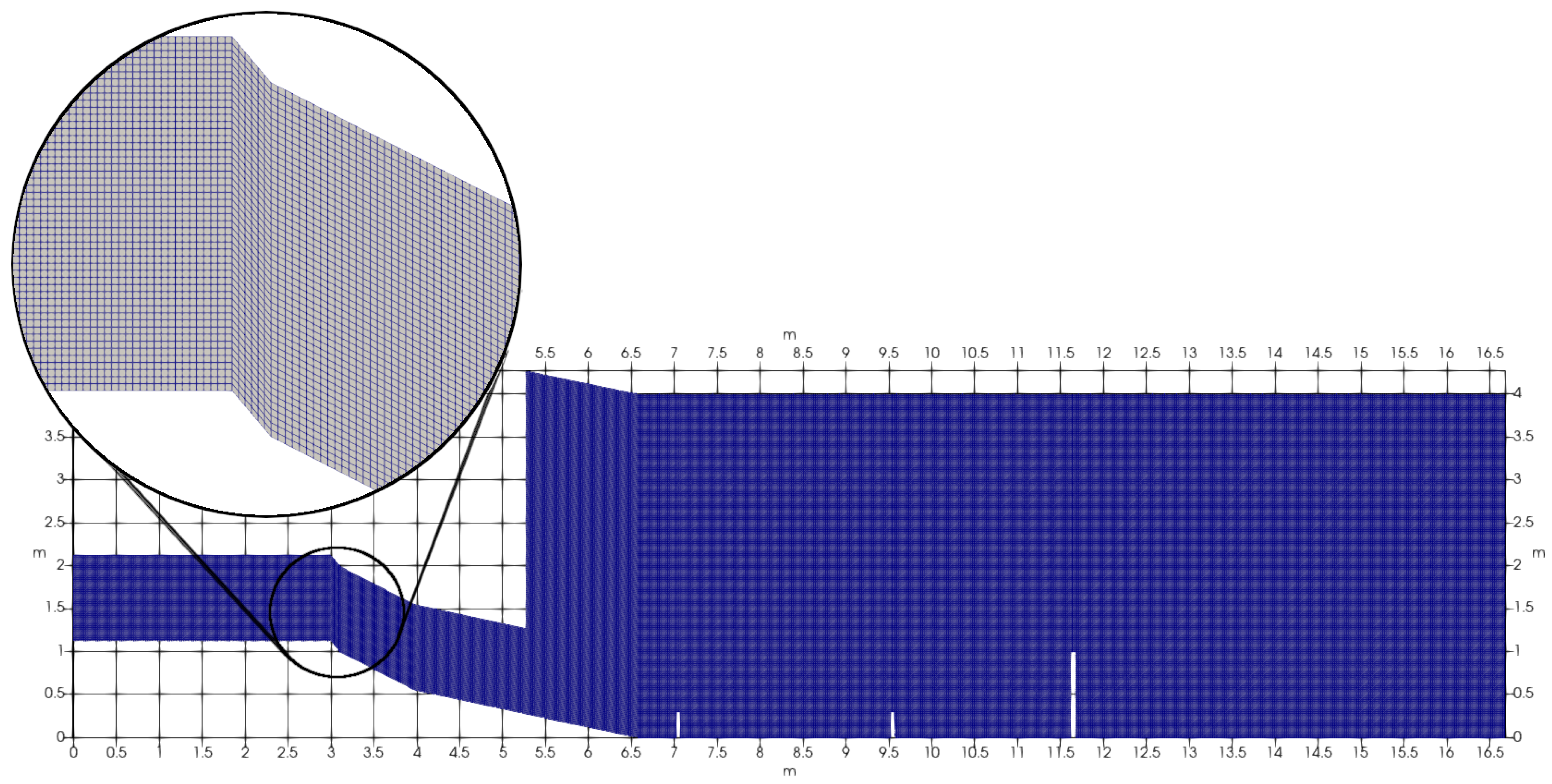
5.3. Computational Mesh for University of Iceland Experiment

To simulate the University of Iceland experiment, a two-dimensional description is used, since the width of the experimental channel is 1 m and the flow depth is about 10 cm. It is reasonable to assume that the side walls do not significantly affect the flow parameters in the middle flow strip where the measurements were made.
The computational domain consists of 254,720 cells. The cells of the mesh are in the form of cubes and parallelepipeds, as shown in the Figure 5.
The solution converges over the mesh. The convergence study was carried out for meshes of 127,360, 254,720, and 509,440 cells.
The following boundaries were determined (Figure 1):
  • the horizontal part of the chute bottom, the reservoir walls, protective structures, end section of the chute are solid walls with the no-slip condition;
  • the inclined parts of the chute bottom: no-slip condition with turbulent rough wall condition with roughness height of 2 mm;
  • computational domain sides: empty boundary condition to implement two-dimensional domain;
  • computational domain upper border: a mixed condition with atmospheric pressure, no inflow through the border and outflow according to zero gradient condition;
At an initial moment of time a 0.9 m depth water column is held in the starting reservoir by a virtual dam, which disappears at the beginning of the calculation.

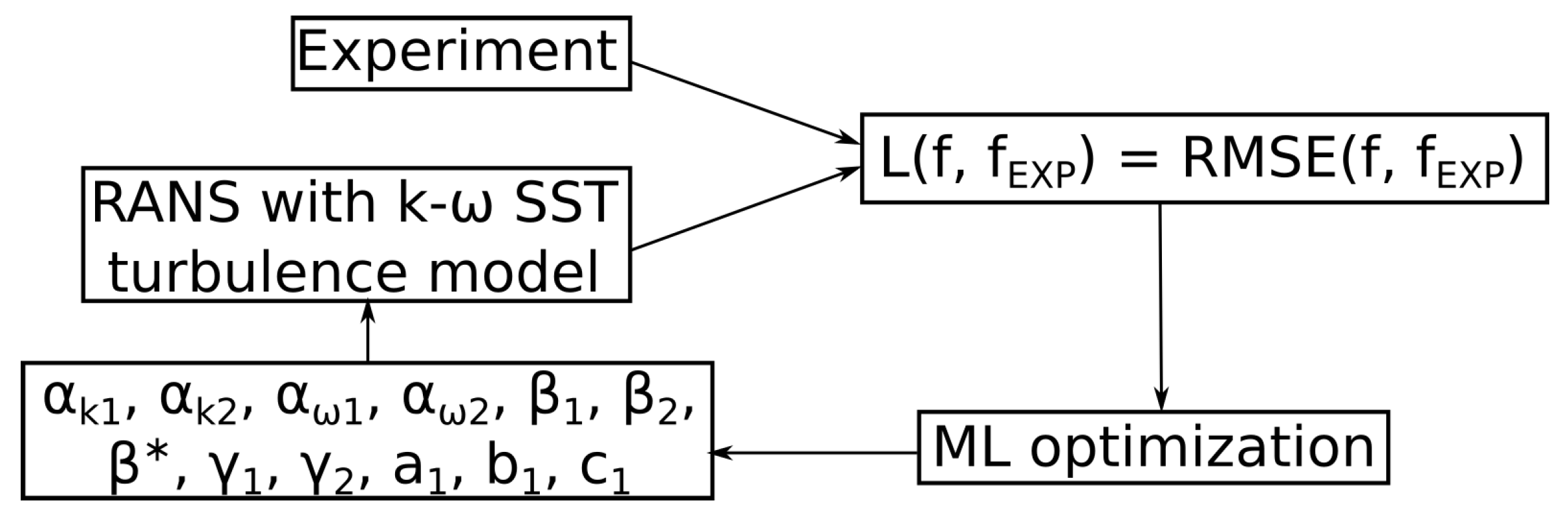
6. Optimization Algorithm

In Section 2 the need to calibrate turbulent models for simulation of free-surface flows on mountain slopes was demonstrated. The efficiency of calibration of the coefficients of turbulence models is shown in [48,49]. Research by Guillas et al. [48] demonstrated the effectiveness of the k- ε turbulence model coefficients calibration for city air flows simulating using Bayesian methods. Ling et al. [49] use deep neural networks trained on high-fidelity simulations to model the Reynolds stress anisotropy tensor in channel flow. The accuracy of modeling the dynamics of avalanches or mudflows is especially important, since it has a strong influence on the design of the protective structures. Without calibration, the difference between the experimental and calculated parameters can reach 50%, as shown in the Table 2.
The standard values of coefficients in the k- ω   S S T turbulence model are:
α k 1 = 0.85 ; α k 2 = 1.0 ; α ω 1 = 0.5 ; α ω 2 = 0.856 ; β 1 = 0.075 ; β 2 = 0.0828 ;
β * = 0.09 ; γ 1 = 5 / 9 ; γ 2 = 0.44 ; a 1 = 0.31 ; b 1 = 1.0 ; c 1 = 10.0 .
In this study the coefficients of the k- ω   S S T model were calibrated using the machine learning algorithm, see Figure 6. The procedure included the following steps:
  • Training of the optimization algorithm based on a Reynolds–Averaged Navier–Stokes equations (RANS) calculations with the k- ω   S S T turbulence model with different constants values;
  • Obtaining new values of the coefficients using the optimization algorithm;
  • Simulation of flow dynamics using obtained turbulence model coefficients;
  • Additional training of the algorithm using the obtained flow dynamics data.
When optimizing the coefficients of the turbulence model, the loss function of the root mean square error (RMSE) of the calculated flow velocity profile in the outlet section from the experimental profile is minimized:
L RMSE = i = 0 N ( v E X P ( i ) v k ω S S T ( i ) ) 2 N .
Here N is the number of points along the normal to the chute bottom in the output section.
The minimization uses the Nelder-Mead method (a multi-variable function optimization method that does not use gradients) implemented in the SciPy library.

Development of an Automatic Optimization Module MLTFoam Optimization

To implement the joint automatic operation of the optimization method and computational fluid dynamics simulation, the MLTFoamOptimization module was developed in Python using the libraries Pandas, NumPy, SciPy, Multiprocessing, Subprocess, PyFoam, etc. The developed module accepts as input the updated values of the coefficients of the turbulent model generated during the optimization process, writes a file with settings for generating a new calculation, and launches the preprocessing utility that prepares the calculation cases. Then the calculations of OpenFOAM cases are started in parallel. Based on the results of the calculations, the value of the loss function is calculated and passed to the optimizer.
The module is available on GitHub along with other utilities necessary for calculating flows on mountain slopes, such as utilities for generating meshes, etc. https://github.com/RomanovaDI/avalancheUtils (accessed on 20 June 2021).

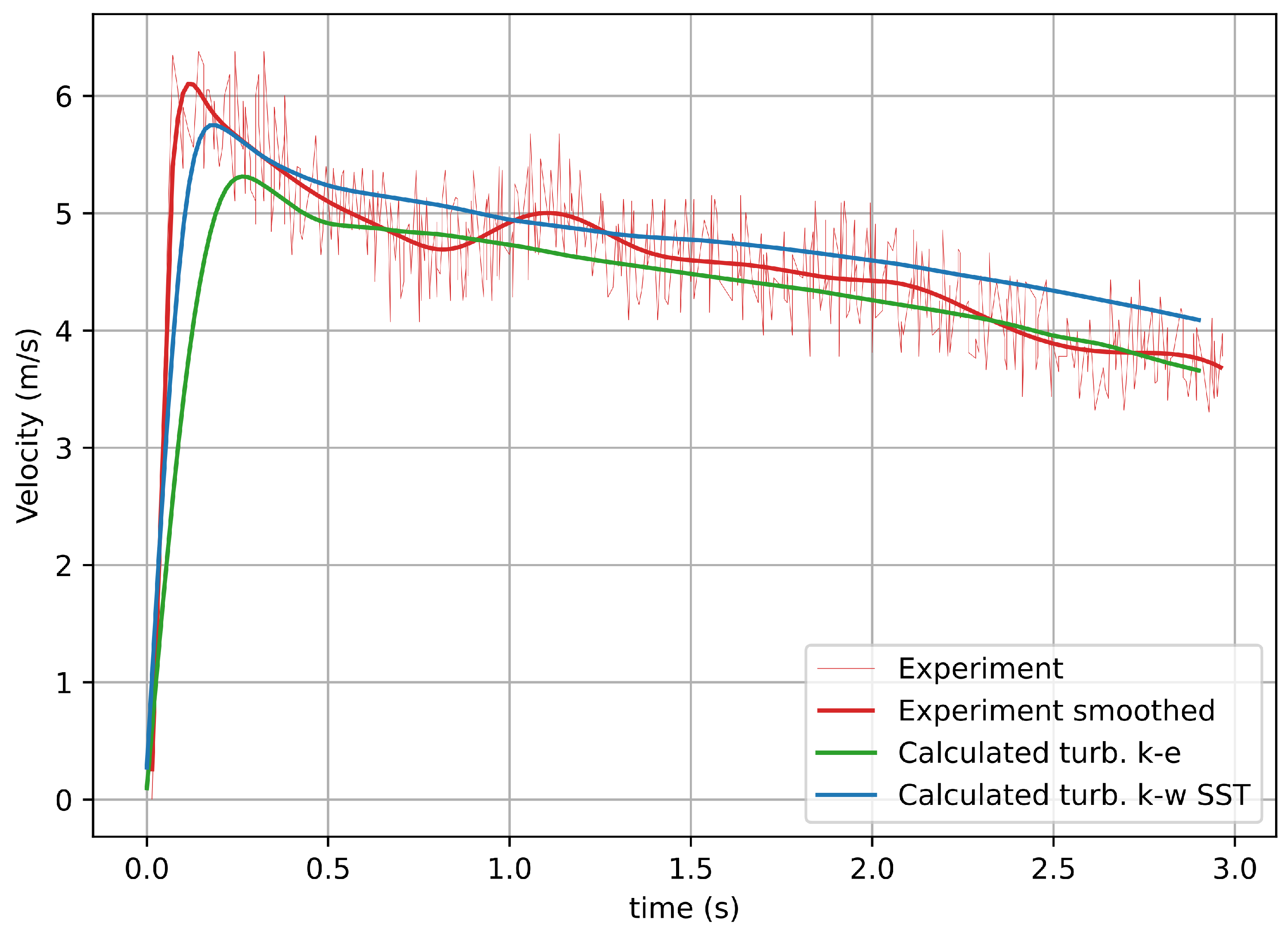
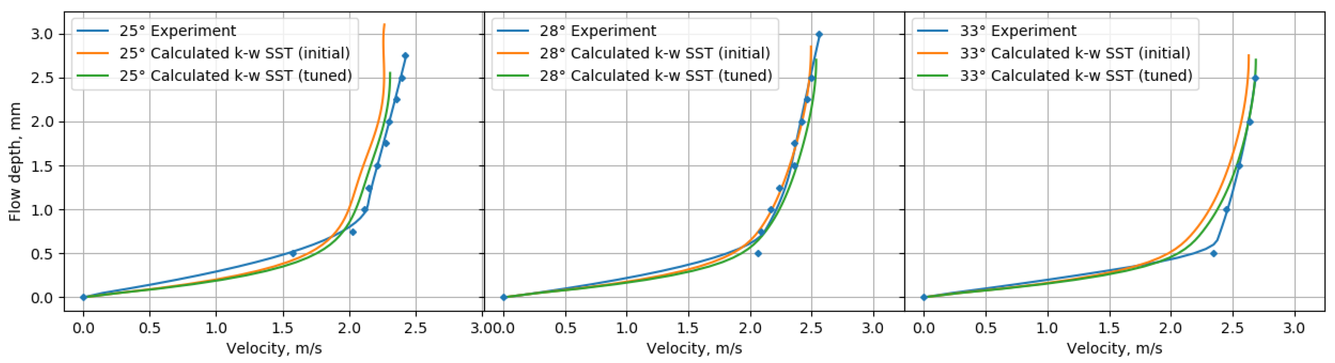
7. Calibration Results

Using the results of an MSU experiment the coefficients of the turbulence model were calibrated. In optimization, the calculated velocity profile tended to be close to the experimental profile.
To optimize the k- ω   S S T turbulence model coefficients 924 calculations of the calibration experiments (Figure 4) were carried out, which took 125 h on 24 cores.
Initial values of the k- ω   S S T turbulence model coefficients:
α k 1 = 0.85 ; α k 2 = 1.0 ; α ω 1 = 0.5 ; α ω 2 = 0.856 ; β 1 = 0.075 ; β 2 = 0.0828 ; β * = 0.09 ; γ 1 = 0.5556 ; γ 2 = 0.44 ; a 1 = 0.31 ; b 1 = 1.0 ; c 1 = 10.0 .
Values of the k- ω   S S T turbulence model coefficients after calibration:
α k 1 = 0.822 ; α k 2 = 1.1304 ; α ω 1 = 0.466 ; α ω 2 = 0.7796 ; β 1 = 0.0852 ; β 2 = 0.0749 ; β * = 0.1131 ; γ 1 = 0.5156 ; γ 2 = 0.4066 ; a 1 = 0.3338 ; b 1 = 0.9508 ; c 1 = 9.8864 .
During the calibration, the following minimization of the loss function (7) was achieved, as shown in Table 4.
Figure 7 compares initial, tuned and experimental velocity profiles in the outlet section for various slope angles.

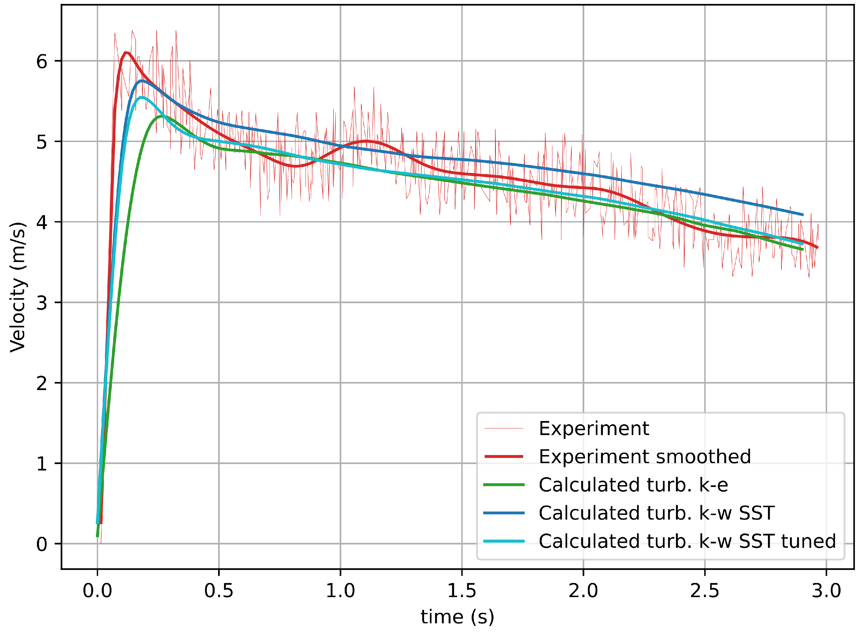
8. Verification of Calibration Results Using the Experiment of the University of Iceland

The UI experiments [38], see Figure 1 and Figure 2, were simulated by the k- ω   S S T turbulence model with the calibrated coefficients. Some results for flows in the presence of three dams are shown in Figure 8 and in Table 5.
The results for a flow in the chute without dams are shown in Figure 9. It shows the decrease in the discrepancy from the experimental data for the flow rate. For the parameters listed in Table 5, we see a decrease in the difference in the height of the initial splash at the main dam from 50% to 15%, the difference in the overflow time of the flow over the main dam decreased from 4% to 1%, for volume of liquid (out of 2.7 m 3 ) retained by the dam in the chute, the difference decreased from 0.8% to 0.3%. Based on the foregoing, we can conclude that the calibration of the coefficients of the turbulence model for the class of problems under study makes it possible to improve the accuracy of calculations.

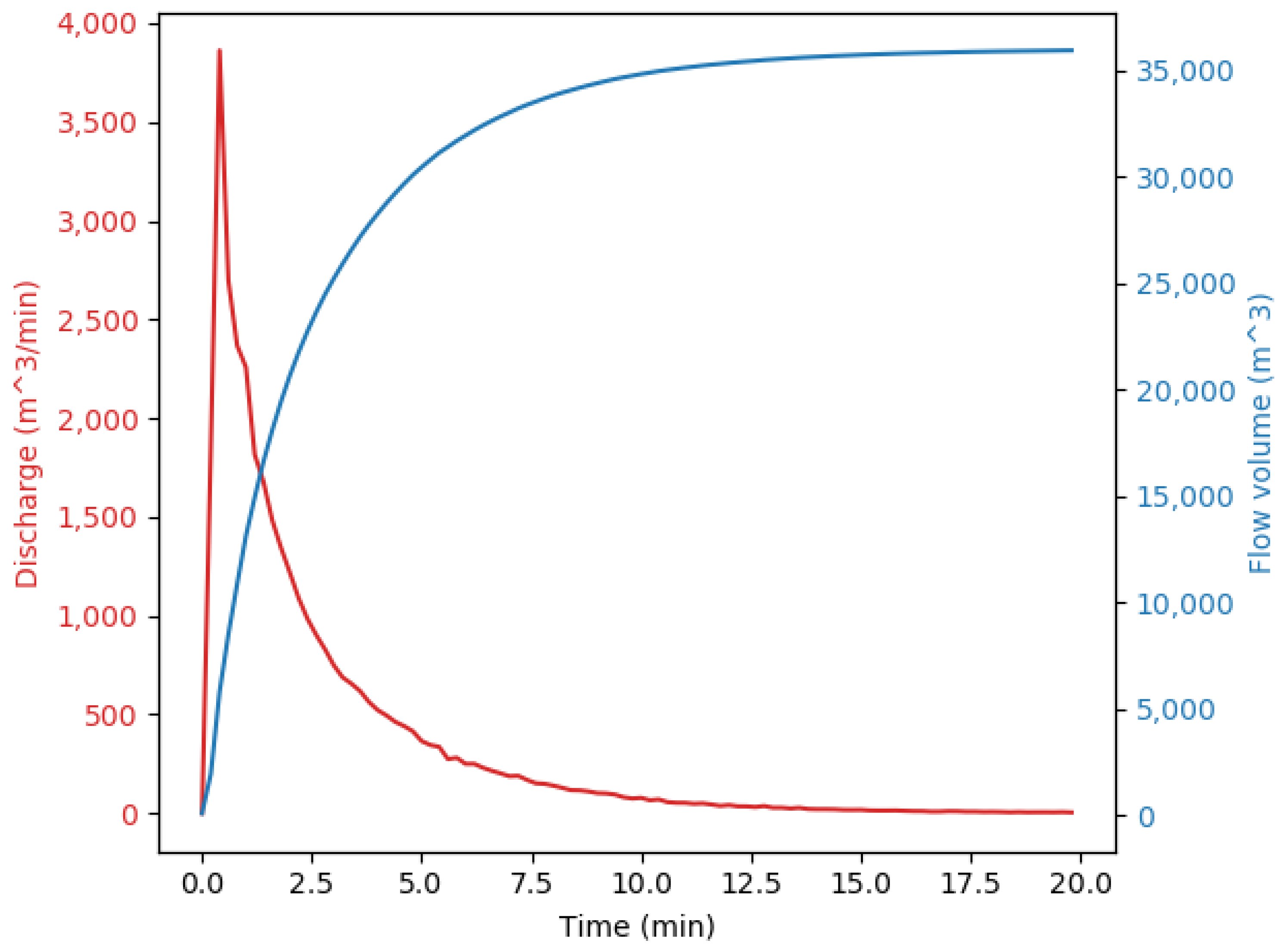
9. Maliy Azau Glacial Lake Outburst Flood

In this section, we provide an example of the application of the developed 3D mathematical model and software for modeling natural mountain currents. Using the k- ω   S S T calibrated turbulence model, a possible outburst of the glacial lake Maliy Azau on Mount Elbrus (Central Caucasus) [50] is simulated.
The group of lakes located near the Maliy Azau glacier on the southern slope of Elbrus is widely known and is annually visited by tourists and climbers. In the period 1957–2021 two cases of lake outburst were recorded: in 1978 and in 2011. The first outburst was associated with the processes of landslide deformations of the moraine massif that composes part of the lake basin, the second with the degradation of the ice dam of the lake and an overflow of water over it.
The developed software allows obtaining the data about the flow path, velocity profiles, pressure distribution in the flow, shear stresses at the bottom of the flow.
At the moment the lake area is about 26 thousand m 2 , lake volume is about 67 thousand m 3 . Simulation of glacial lake outburst flood was carried out. Some results are shown in Figure 10 and Figure 11. On the left part of Figure 10 the map of the studied area is shown [50], the contour of the computational area is schematically marked in green; on the right the 3D simulation of outburst flood is shown 1 min after start, flow is colored according to the magnitude of the velocity (right).
In Figure 11 it is shown that the lake outburst lasts about 20 min, the maximum flow rate is about 4000 m 3 /min. The total outflow water volume is about 35,000 m 3 . In addition, the Figure 11 shows an increase in fluid flow with further leveling, which is typical for outburst floods of glacial lakes.
It should be noted that the results obtained in this Section give only some rough estimates of the flow parameters during the breakthrough flood. For more accurate modeling, it is necessary to additionally take into account a number of factors that can significantly affect the flow dynamics. In particular, one of the important factors is the possible erosion of the bottom by the current and the entrainment of bottom material, which are not taken into account in the mathematical model used in this study.

10. Results and Conclusions

This article is devoted to the problem of three-dimensional modeling of dense turbulent flows on slopes. In particular, our goal was to find out whether the coefficients of the k- ω   S S T turbulence model can be calibrated to simulate such flows. To this end, we considered two experimental studies of water flows in experimental chutes with dams located in the flow path. One of these studies was carried out in the University of Iceland, the other—at the Institute of Mechanics of the Lomonosov Moscow State University using an experimental setup created by the authors of this article.
First, the flows measured in these two studies were simulated by the standard k- ω   S S T turbulent model using the free OpenFOAM software package, and a certain discrepancy was found between some of the measured and simulated flow parameters.
Secondly, additional modules for OpenFOAM package has been developed, which are necessary for organize the calibration of the model coefficients, including the machine learning approach. These additions to the standard package have been posted online to make them available to everyone.
Thirdly, a special experimental setup at the Institute of Mechanics of Lomonosov Moscow State University has been done and the flow parameters needed to calibrate the turbulence model has been measure.
Then the coefficients of the turbulence model were calibrated using the experimental results obtained by the authors at the MSU experimental chute. Three series of experiments were used, which made it possible to avoid algorithm overfitting. As a result, some values of the model coefficients were adjusted.
Finally, simulations of the experiments at UI including the interaction with the dams was performed using the adjusted model coefficients. The results are in better agreement with the experimental data; therefore, coefficients calibration is useful.
At the same time, the discrepancy between some of the measured and calculated parameters was still quite significant. In this article, we do not discuss the reasons, possibly related to a simplified formulation of the problem or the computational methods used. The main content of this article is the development of a method for calibrating the coefficients of the turbulence model and the demonstration of the calibration results. It is worth to note that for the considered water flows, the increase in modeling accuracy due to calibration turned out to be relatively small. However, the method developed here can be useful for finding model coefficients for more complex flows, in particular, for flows with non-Newtonian rheological properties.
The last section of the article describes the modeling of the flow resulting from the breakthrough of the glacial lake Maliy Azau (Elbrus, Central Caucasus), taking into account the real topography of the slope. In recent years, there have been two real breakthroughs of the lake, but, unfortunately, no measurements of the path and flow parameters were carried out. Since the surroundings of the lake are very popular with tourists and climbers, information on the parameters of possible outburst floods is important. The results in this section provide some information. However, it should be emphasized once more that this information presents only some rough estimates of the flow parameters during a breakthrough flood since a number of factors that can significantly affect the flow dynamics have not been taken into account, e.g., possible entrainment of bottom material.
It is important to note that only water flows were modeled in this paper, while most flows on mountain slopes are flows of non-Newtonian fluids. The study of the applicability of the known turbulence models and, in particular, the dependence of the model coefficients on the rheological properties of the moving medium, can be carried out using the calibration algorithms developed here. Unfortunately, it is currently impossible to do this due to the lack of detailed experimental data on turbulent slope non-Newtonian flows. Another important process to consider when simulating slope flows is the underlying material entrainment. Simulations taking into account the complex rheological properties of the flow and the entrainment of material from the slope are planned for the future.

Author Contributions

D.R., O.I., V.T., N.G., D.K., B.G. and N.K. jointly constructed and carried out a turbulent slope flow experiment in the Research Institute of Mechanics of Moscow State University. D.R. carried out simulations of experiments and calibration of the turbulent model and wrote the text of the paper. N.G. and D.K. analyzed the problem of outburst of a lake near the glacier Maliy Azau on the Elbrus (Central Caucasus). M.E. and S.S. supervised the research team. All authors have read and agreed to the published version of the manuscript.

Funding

The reported study was funded by RFBR, project number 19-31-90105.

Institutional Review Board Statement

Not applicable.

Informed Consent Statement

Not applicable.

Data Availability Statement

The optimization algorithm, pre- and post-processing utilities necessary for calculating flows on mountain slopes are available on GitHub https://github.com/RomanovaDI/avalancheUtils (accessed on 20 June 2021).

Acknowledgments

The authors are very grateful to Dieter Issler, whose numerous significant comments helped to improve essentially the quality of this paper. Thanks the anonymous reviewers for their useful comments. Thanks to Project Sirius. Summer for experiment organizing.

Conflicts of Interest

The authors declare no conflict of interest. The funders had no role in the design of the study; in the collection, analyses, or interpretation of data; in the writing of the manuscript, or in the decision to publish the results.

References

  1. Briukhanov, A.; Grigorian, S.; Miagkov, S.; Plam, M.; Shurova, I.; Eglit, M.; Yakimov, Y. On some new approaches to the dynamics of snow avalanches. Phys. Snow Ice 1966, 1, 1223–1241. [Google Scholar]
  2. Grigorian, S.S.; Eglit, M.E.; Iakimov, Y.L. A new formulation and solution of the problem of snow avalanche motion. Tr. Vycokogornogo Geofiz. Inst. 1967, 12, 104–113. [Google Scholar]
  3. Eglit, M. Theoretical approaches to the calculation of the motion of snow avalanches. Itogi Nauki 1968, 60–97. [Google Scholar]
  4. Bakhvalov, N.; Eglit, M. Study of the solutions of equations of motion of snow avalanches. Mater. Glyatsiologicheskikh Issled. (Data Glaciol. Stud.) 1970, 16, 7–14. [Google Scholar]
  5. Eglit, M. Some Mathematical Models of Snow Avalanches. Adv. Mech. Flow Granul. Mater. 1983, 2, 557–588. [Google Scholar]
  6. Eglit, M. Calculation of the parameters of avalanches in the runout zone. Mater. Glyatsiologicheskikh Issled. (Data Glaciol. Stud.) 1982, 53, 35–39. [Google Scholar]
  7. Savage, S.B.; Hutter, K. The motion of a finite mass of granular material down a rough incline. J. Fluid Mech. 1989, 199, 177–215. [Google Scholar] [CrossRef]
  8. Kulikovskii, A.; Eglit, M. Two-dimensional problem of the motion of a snow avalanche along a slope with smoothly changing properties. J. Appl. Math. Mech. 1973, 37, 792–803. [Google Scholar] [CrossRef]
  9. Eglit, M. Unsteady Motions in Channels and on Slopes; MSU Press: Moscow, Russia, 1986. [Google Scholar]
  10. Mironova, E. Mathematical Modelling of the Motion of Water Flows, Snow Avalanches, and Floods. Ph.D. Thesis, Lomonosov Moscow State University, Moscow, Russia, 1987. [Google Scholar]
  11. Volodicheva, N.; Mironova, E.; Oleinikov, A.; Eglit, M. The use of mathematical modelling to determine the boundaries of propagation of avalanches. Mater. Glyatsiologicheskikh Issled. (Data Glaciol. Stud.) 1986, 56, 78–81. [Google Scholar]
  12. Christen, M.; Kowalski, J.; Bartelt, P. RAMMS: Numerical simulation of dense snow avalanches in three-dimensional terrain. Cold Reg. Sci. Technol. 2010, 63, 1–14. [Google Scholar] [CrossRef] [Green Version]
  13. Bühler, Y.; Christen, M.; Kowalski, J.; Bartelt, P. Sensitivity of snow avalanche simulations to digital elevation model quality and resolution. Ann. Glaciol. 2011, 52, 72–80. [Google Scholar] [CrossRef] [Green Version]
  14. Christen, M.; Bartelt, P.; Kowalski, J.; Stoffel, L. Calculation of dense snow avalanches in three-dimensional terrain with the numerical simulation program RAMMS. In Proceedings of the Whistler 2008 International Snow Science Workshop, Whistler, BC, Canada, 21–27 September 2008. [Google Scholar]
  15. Fischer, J.T.; Kowalski, J.; Pudasaini, S.; Miller, S. Dynamic Avalanche Modeling in Natural Terrain. In Proceedings of the International Snow Science Workshop, Davos, Switzerland, 27 September–2 October 2009. [Google Scholar]
  16. Pitman, E.B.; Nichita, C.C.; Patra, A.; Bauer, A.; Sheridan, M.; Bursik, M. Computing granular avalanches and landslides. Phys. Fluids 2003, 15, 3638–3646. [Google Scholar] [CrossRef] [Green Version]
  17. Patra, A.; Bauer, A.; Nichita, C.; Pitman, E.; Sheridan, M.; Bursik, M.; Rupp, B.; Webber, A.; Stinton, A.; Namikawa, L.; et al. Parallel adaptive numerical simulation of dry avalanches over natural terrain. J. Volcanol. Geotherm. Res. 2005, 139, 1–21. [Google Scholar] [CrossRef]
  18. Mousavi Tayebi, S.A.; Moussavi Tayyebi, S.; Pastor, M. Depth-Integrated Two-Phase Modeling of Two Real Cases: A Comparison between r.avaflow and GeoFlow-SPH Codes. Appl. Sci. 2021, 11, 5751. [Google Scholar] [CrossRef]
  19. Naaim, M.; Gurer, I. Two-phase numerical model of powder avalanche: Theory and application. Nat. Hazards 1998, 117, 129–145. [Google Scholar] [CrossRef]
  20. Sampl, P.; Zwinger, T. Avalanche simulation with SAMOS. Ann. Glaciol. 2004, 38, 393–398. [Google Scholar] [CrossRef] [Green Version]
  21. Hermann, F.; Issler, D.; Keller, S. Towards a numerical model of powder snow avalanches. In Computational Fluid Dynamics’ 94; Wiley: Chichester, NY, USA, 1994; pp. 948–955. [Google Scholar]
  22. Yamaguchi, Y.; Takase, S.; Moriguchi, S.; Terada, K.; Oda, K.; Kamiishi, I. Three-dimensional nonstructural finite element analysis of snow avalanche using non-Newtonian fluid model. Trans. Jpn. Soc. Comput. Eng. Sci. 2017, 2017, 20170011. [Google Scholar] [CrossRef]
  23. Oda, K.; Moriguchi, S.; Kamiishi, I.; Yashima, A.; Sawada, K.; Sato, A. Simulation of a snow avalanche model test using computational fluid dynamics. Ann. Glaciol. 2011, 52, 57–64. [Google Scholar] [CrossRef] [Green Version]
  24. Romanova, D.I. 3D avalanche flow modeling using OpenFOAM. Proc. ISP RAS 2017, 29, 85–100. [Google Scholar] [CrossRef] [Green Version]
  25. Romanova, D. Comparison of Single-Velocity and Multi-Velocity Multiphase Models for Slope Flow Simulations. In Proceedings of the 2020 Ivannikov Ispras Open Conference (ISPRAS), Moscow, Russia, 10–11 December 2020; pp. 170–174. [Google Scholar] [CrossRef]
  26. Scheiwiller, T. Dynamics of Powder-Snow Avalanches. Ph.D. Thesis, ETH Zurich, Zürich, Switzerland, 1986. [Google Scholar] [CrossRef]
  27. Brandstatter, W.; Hagen, F.; Sampl, P.; Schaffhauser, H. Dreidimensionalle Simulation von Staublawinen unter Berucksichtigung realer Gelandeformen. Z. Der-Wildbach- Lawinebnverbauung Osterreichs 1992, 120, 107–137. [Google Scholar]
  28. Sampl, P. Current status of the AVL Avalanche Simulation Model—Numerical simulation of dry snow avalanches. In Proceedings of the “Pierre Beghin” International Workshop On Rapid Gravitational Mass Movements, Grenoble, France, 6–10 December 1993; Volume 1, pp. 269–296. [Google Scholar]
  29. Menter, F. Zonal Two Equation k-w Turbulence Models For Aerodynamic Flows. In Proceedings of the 23rd Fluid Dynamics, Plasmadynamics, and Lasers Conference, Nashville, TN, USA, 6–8 July 1992. [Google Scholar] [CrossRef]
  30. Menter, F.R. Two-equation eddy-viscosity turbulence models for engineering applications. AIAA J. 1994, 32, 1598–1605. [Google Scholar] [CrossRef] [Green Version]
  31. Menter, F.; Kuntz, M.; Langtry, R. Ten years of industrial experience with the SST turbulence model. Heat Mass Transf. 2003, 4, 1–8. [Google Scholar]
  32. Kalitzin, G.; Medic, G.; Xia, G. Improvements to SST turbulence model for free shear layers, turbulent separation and stagnation point anomaly. In Proceedings of the 54th AIAA Aerospace Sciences Meeting, San Diego, CA, USA, 4–8 January 2016; p. 1601. [Google Scholar]
  33. Rocha, P.C.; Rocha, H.B.; Carneiro, F.M.; da Silva, M.V.; de Andrade, C.F. A case study on the calibration of the k-ω SST (shear stress transport) turbulence model for small scale wind turbines designed with cambered and symmetrical airfoils. Energy 2016, 97, 144–150. [Google Scholar] [CrossRef]
  34. Rocha, P.; Rocha, H.; Carneiro, F.; Silva, M.; Bueno, A. K-ω SST (shear stress transport) turbulence model calibration: A case study on a small scale horizontal axis wind turbine. Energy 2013, 65, 412–418. [Google Scholar] [CrossRef]
  35. Launder, B.; Spalding, D. The numerical computation of turbulent flows. Comput. Methods Appl. Mech. Eng. 1974, 103, 456–460. [Google Scholar] [CrossRef]
  36. Tahry, S.H.E. k-epsilon equation for compressible reciprocating engine flows. J. Energy 1983, 7, 345–353. [Google Scholar] [CrossRef]
  37. Launder, B.; Morse, A.; Rodi, W.; Spaldiug, D. Spaldiug, The prediction of free shear flows—A comparison of the performance of six turbulence models. In Proceedings of the NASA Conference on Free Shear Flows, Hampton, VA, USA, 20–21 July 1972. [Google Scholar]
  38. Agustsdottir, K.H. The Design of Slushflow Barriers: Laboratory Experiments. Ph.D. Thesis, University of Iceland, Reykjavik, Iceland, 2019. [Google Scholar]
  39. Jones, R.A. The Design of Slushflow Barriers: CFD Simulations. Ph.D. Thesis, University of Iceland, Reykjavik, Iceland, 2019. [Google Scholar]
  40. Romanova, D. Architecture of Open Source Program for Numerical Modeling of Flows on Mountain Slopes. Proc. Inst. Syst. Program. Ras (Proc. ISP RAS) 2020, 32, 183–200. [Google Scholar] [CrossRef]
  41. Ferziger, J.; Peric, M. Computational Methods for Fluid Dynamics; Springer: Berlin/Heidelberg, Germany, 2002; Volume 3. [Google Scholar] [CrossRef]
  42. Berberovic, E.; van Hinsberg, N.P.; Jakirlic, S.; Roisman, I.V.; Tropea, C. Drop impact onto a liquid layer of finite thickness: Dynamics of the cavity evolution. Phys. Rev. E 2009, 79, 036306. [Google Scholar] [CrossRef] [PubMed]
  43. Rusche, H. Computational Fluid Dynamics of Dispersed Two-Phase Flows at High Phase Fractions. Ph.D. Thesis, University of London, London, UK, 2002. [Google Scholar]
  44. Hirt, C.; Nichols, B. Volume of fluid (VOF) method for the dynamics of free boundaries. J. Comput. Phys. 1981, 39, 201–225. [Google Scholar] [CrossRef]
  45. Ubbink, O. Numerical Prediction of Two Fluid Systems with Sharp Interfaces. Ph.D. Thesis, Department of Mechanical Engineering, Imperial College of Science, Technology & Medicine, London, UK, 1997. [Google Scholar]
  46. Holzmann, T. Mathematics, Numerics, Derivations and OpenFOAM®; Holzmann CFD: Loeben, Germany, 2019. [Google Scholar]
  47. Yin, R. Comparison of four algorithms for solving pressure-velocity linked equations in simulating atrium fire. Int. J. Archit. Sci. 2003, 4, 24–35. [Google Scholar]
  48. Guillas, S.; Glover, N.; Malki-Epshtein, L. Bayesian calibration of the constants of the k-ε turbulence model for a CFD model of street canyon flow. Comput. Methods Appl. Mech. Eng. 2014, 279, 536–553. [Google Scholar] [CrossRef] [Green Version]
  49. Ling, J.; Kurzawski, A.; Templeton, J. Reynolds averaged turbulence modelling using deep neural networks with embedded invariance. J. Fluid Mech. 2016, 807, 155–166. [Google Scholar] [CrossRef]
  50. Dokukin, M.; Khatkutov, A. Lakes near the glacier Maliy Azau on the Elbrus (Central Caucasus): Dynamics and outbursts. Ice Snow 2016, 56, 472–479. [Google Scholar] [CrossRef]
Figure 1. Scheme of chute in University of Iceland experiment.
Fluids 07 00111 g001
Figure 2. Calculation domain and initial condition for simulating the experiment at the University of Iceland experiment chute. The green line shows the location of the section in which the data was measured and calculated for the flow without dams.
Fluids 07 00111 g002
Figure 3. The flow without dams. Depth-averaged velocity at a distance of 11.1 m from the beginning of the chute. Red lines—experiment [38]; green line—simulated by k- ε turbulence model; blue line—simulated by the k- ω S S T turbulence model.
Fluids 07 00111 g003
Figure 4. Experiment chute scheme.
Fluids 07 00111 g004
Figure 5. Calculation mesh for University of Iceland experiment chute.
Fluids 07 00111 g005
Figure 6. The architecture of the proposed algorithm for calibrating the k- ω S S T turbulence model coefficients.
Fluids 07 00111 g006
Figure 7. Comparison of velocity profiles calculated by the k- ω S S T model using initial and tuned coefficients with the experimental profile at different chute inclination angles.
Fluids 07 00111 g007
Figure 8. The interaction of the flow with three dams (simulation). There are splashes and formation of jets on the dams. The colors are related to the values of α (i.e., the relative part of the cell occupied by liquid): blue—1, black—0. White lines are dams.
Fluids 07 00111 g008
Figure 9. Depth-averaged velocity measured at a distance of 11.1 m from the beginning of the chute without dams. The water boundary is defined by a water volume fraction of 90%. The experimental data taken from [38] (Experiment) colored in red, calculated data obtained by the authors using the k- ε turbulence model (Calculated k-ε) colored in green, calculated data obtained by the authors using the k- ω S S T turbulence model (Calculated k-ω SST) colored in blue and calculated data obtained by the authors using the k- ω S S T turbulence model (Calculated k-ω SST tuned) with tuned coefficients colored in cyan.
Fluids 07 00111 g009
Figure 10. Maliy Azau glacial lake outburst flood map [50] (left); 3D simulation of outburst flood 1 minute after start (right).
Fluids 07 00111 g010
Figure 11. Discharge (red) and the volume of liquid poured out of the lake (blue) versus time from the start of the outburst.
Fluids 07 00111 g011
Table 1. Parameters of flows in study.
ParametersMSU ExperimentUI ExperimentMaliy Azau GLOF
Density, ρ [ kg / m 3 ]100010001000
Average velocity, u a v [ m / s ]2.5110
Flow path length, L [m]0.5151500
Average depth, h a v [m]0.0040.10.1
Average slope angle, θ a v 30 15 25
Viscosity, ν [ m 2 / s ] 10 6 10 6 10 6
Reynolds number, Re = u a v h a v ν 10 4 10 5 10 6
Table 2. Comparison of measured and calculated parameters for a flow in a chute with three dams.
Comparison ParameterExperiment [38]Simulations
k - ε Model k - ω SSTModel
Height of initial splash on main dam1.3 m1.61 m1.95 m
Overflow time of the flow over the main dam1.25 s1.3 s1.3 s
Volume of liquid (of 2.7 m 3 ) retained by the dam2.684 m 3 2.650 m 3 2.635 m 3
Table 3. Parameters of the experiments.
u 0 (Depth-Averaged), m/s h 0 , mm θ Fr = u 0 / g h 0
1.634.2025 8.03
2.004.9528 9.08
1.783.4533 9.68
Table 4. Loss function minimization.
Slope AngleInitial Value of Loss FunctionMinimized Value of Loss Function
25 0.1650.154
28 0.0850.082
33 0.1500.124
Table 5. Comparison of measured and calculated flow parameters in the presence of three dams.
Comparison ParameterExperiment DataCalculation Data
k - ε Turbulence Model k - ω SST Turbulence ModelTuned k - ω SST Turbulence Model
Height of initial splash on main dam1.3 m1.61 m1.95 m1.5 m
Overflow time of the flow over the main dam1.25 s1.3 s1.3 s1.26 s
Volume of liquid (of 2.7 m 3 ) retained by the dam2.684 m 3 2.650 m 3 2.635 m 3 2.676 m 3
Publisher’s Note: MDPI stays neutral with regard to jurisdictional claims in published maps and institutional affiliations.

