
Efficient Reduced Order Modeling of Large Data Sets Obtained from CFD Simulations


Abstract
:1. Introduction
2. Materials and Methods
3. Results and Discussion
3.1. Time-Averaged Flow Field
3.2. ROM of the Full Data Set
3.3. ROM of the Reduced Data Sets
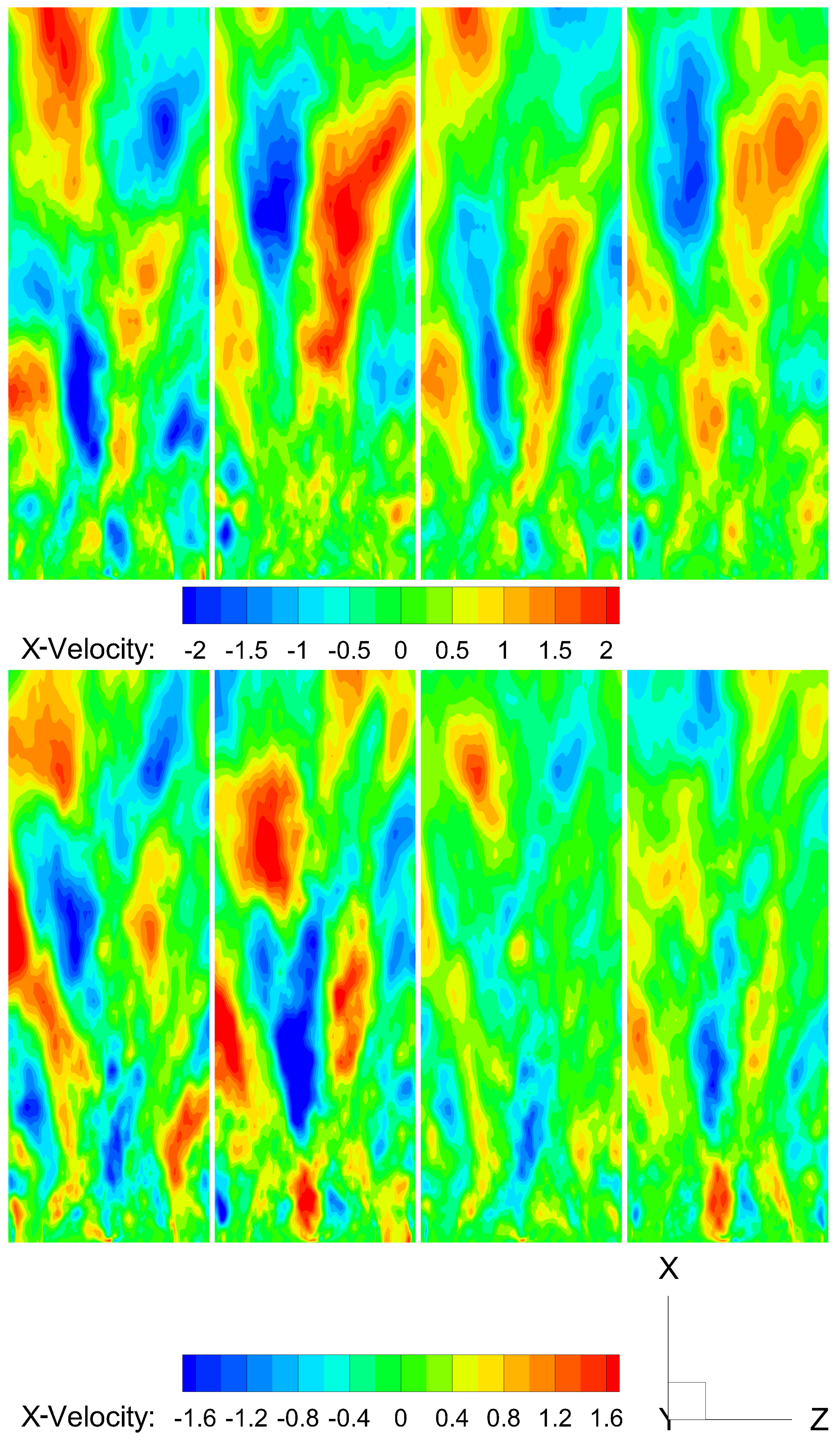
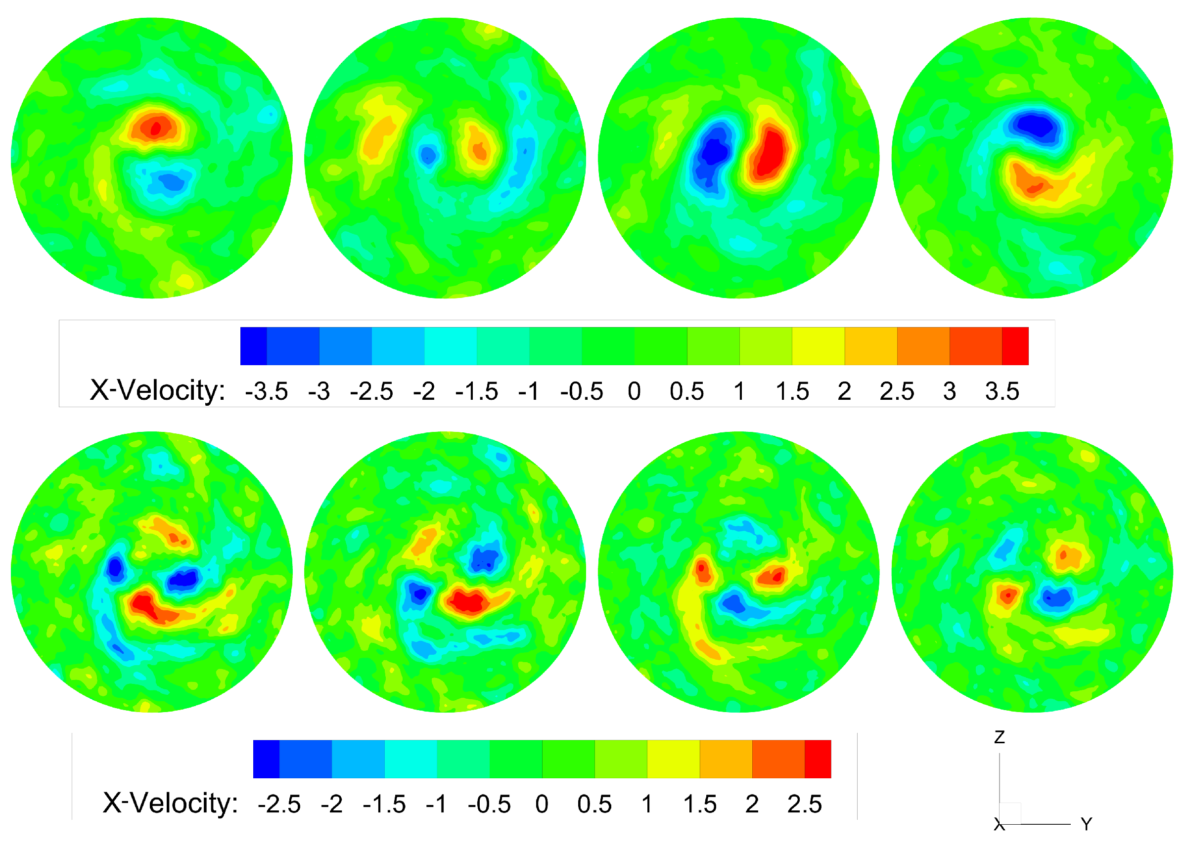
3.4. 3D Spatial Mode Reconstruction from 2D ROM
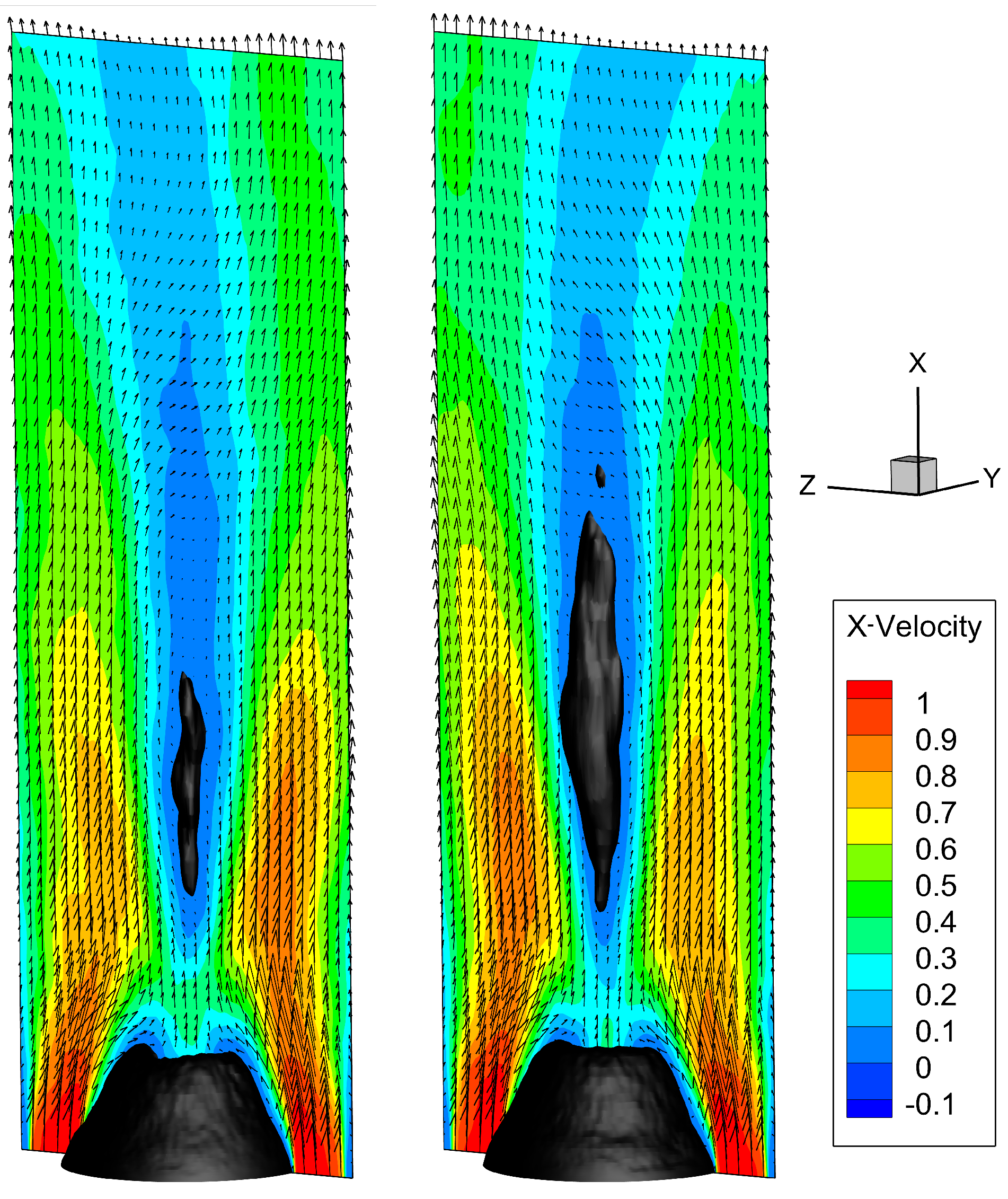
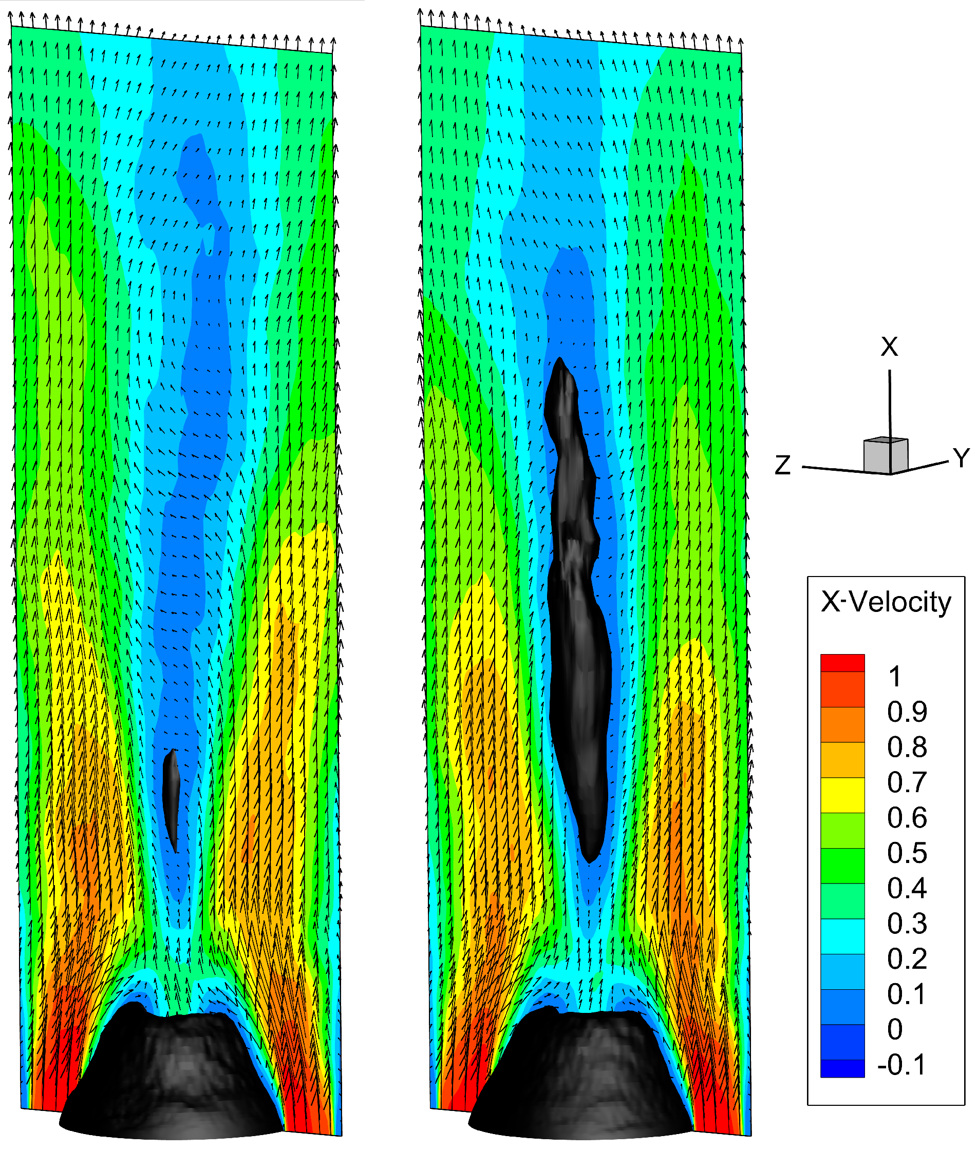
3.5. Flow Field Reconstruction of Low-Frequency Coherent Structures
4. Conclusions
Author Contributions
Funding
Institutional Review Board Statement
Informed Consent Statement
Data Availability Statement
Acknowledgments
Conflicts of Interest
References
- Greco, C.S.; Paolillo, G.; Astarita, T.; Cardone, G. The von Karman street behind a circular cylinder: Flow control through synthetic jet placed at the rear stagnation point. J. Fluid Mech. 2020, 901, A39. [Google Scholar] [CrossRef]
- Wang, F.; Lam, K.M. Experimental and numerical investigation of turbulent wake flow around wall-mounted square cylinder of aspect ratio 2. Exp. Therm. Fluid Sci. 2021, 123, 110325. [Google Scholar] [CrossRef]
- Motoori, Y.; Goto, S. Hairpin vortices in the largest scale of turbulent boundary layers. Int. J. Heat Fluid Flow 2020, 86, 108658. [Google Scholar] [CrossRef]
- Vanierschot, M.; Müller, J.; Sieber, M.; Percin, M.; Van Oudheusden, B.; Oberleithner, K. Single- and double-helix vortex breakdown as two dominant global modes in turbulent swirling jet flow. J. Fluid Mech. 2020, 883, A31. [Google Scholar] [CrossRef]
- Sharaborin, D.K.; Savitskii, A.G.; Bakharev, G.Y.; Lobasov, A.S.; Chikishev, L.M.; Dulin, V.M. PIV/PLIF investigation of unsteady turbulent flow and mixing behind a model gas turbine combustor. Exp. Fluids 2021, 62, 96. [Google Scholar] [CrossRef]
- Vanierschot, M.; Percin, M.; van Oudheusden, B.W. Asymmetric vortex shedding in the wake of an abruptly expanding annular jet. Exp. Fluids 2021, 62, 77. [Google Scholar] [CrossRef]
- Tiwari, S.S.; Bale, S.; Patwardhan, A.W.; Nandakumar, K.; Joshi, J.B. Insights into the physics of dominating frequency modes for flow past a stationary sphere: Direct numerical simulations. Phys. Fluids 2019, 31, 045108. [Google Scholar] [CrossRef]
- Zhang, Y.; Vanierschot, M. Determination of single and double helical structures in a swirling jet by spectral proper orthogonal decomposition. Phys. Fluids 2021, 33, 015115. [Google Scholar] [CrossRef]
- Lumley, J.L. Stochastic Tools in Turbulence. Applied Mathematics and Mechanics Series: Volume 12; Academic Press: New York, NY, USA, 1970. [Google Scholar]
- Sirovich, L. Turbulence and the dynamics of coherent structures. Part I: Coherent structures. Quat. Appl. Math. 1987, 45, 561–571. [Google Scholar] [CrossRef] [Green Version]
- Boreé, J. Extended proper orthogonal decomposition: A tool to analyse correlated events in turbulent flows. Exp. Fluids 2003, 35, 188–192. [Google Scholar] [CrossRef]
- Schmid, P.J. Dynamic mode decomposition of numerical and experimental data. J. Fluid Mech. 2010, 656, 5–28. [Google Scholar] [CrossRef] [Green Version]
- Williams, M.O.; Kevrekidis, I.G.; Rowley, C.W. A Data-Driven Approximation of the Koopman Operator: Extending Dynamic Mode Decomposition. J. Nonlinear Sci. 2015, 25, 1307–1346. [Google Scholar] [CrossRef] [Green Version]
- Sieber, M.; Paschereit, C.O.; Oberleithner, K. Spectral Proper Orthogonal Decomposition. Fluid Mech. 2016, 792, 798–828. [Google Scholar] [CrossRef] [Green Version]
- Gadalla, M.; Cianferra, M.; Tezzele, M.; Stabile, G.; Mola, A.; Rozza, G. On the Comparison of LES Data-Driven Reduced Order Approaches for Hydroacoustic Analysis. Comput. Fluids 2021, 216, 104819. [Google Scholar] [CrossRef]
- Hall, B.T.; Chou, C.-S.; Chen, J.-P. Using the Nonuniform Dynamic Mode Decomposition to Reduce the Storage Required for PDE Simulations. Int. J. Aerosp. Eng. 2019, 2019, 8291616. [Google Scholar] [CrossRef] [Green Version]
- Sieber, M.; Paschereit, C.O.; Oberleithner, K. Advanced Identification of Coherent Structures in Swirl-Stabilized Combustors. J. Eng. Gas Turbine Power 2017, 139, 021503. [Google Scholar] [CrossRef]
- Zixiang, C. Large-Scale Coherent Structures and Three-Dimensional Velocity Estimation in the Turbulent Wake of a Low Aspect Ratio Surface-Mountede Cone. Ph.D. Thesis, University of Calgary, Calgary, AB, Canada, 2017. [Google Scholar]
- Vázquez, J.A.R. A Computational Fluid Dynamics Investigation of Turbulent Swirling Burners. Ph.D. Thesis, Universidad De Zaragoza, Zaragoza, Spain, 2012. [Google Scholar]
- Zhang, Y.; Vanierschot, M. Modeling capabilities of unsteady RANS for the simulation of turbulent swirling flow in an annular bluff-body combustor geometry. Appl. Math. Mod. 2020, 89, 1140–1154. [Google Scholar] [CrossRef]
- Vanierschot, M.; Ogus, G. Experimental investigation of the precessing vortex core in annular swirling jet flows in the transitional regime. Exp. Therm. Fluid Sc. 2019, 106, 148–158. [Google Scholar] [CrossRef]


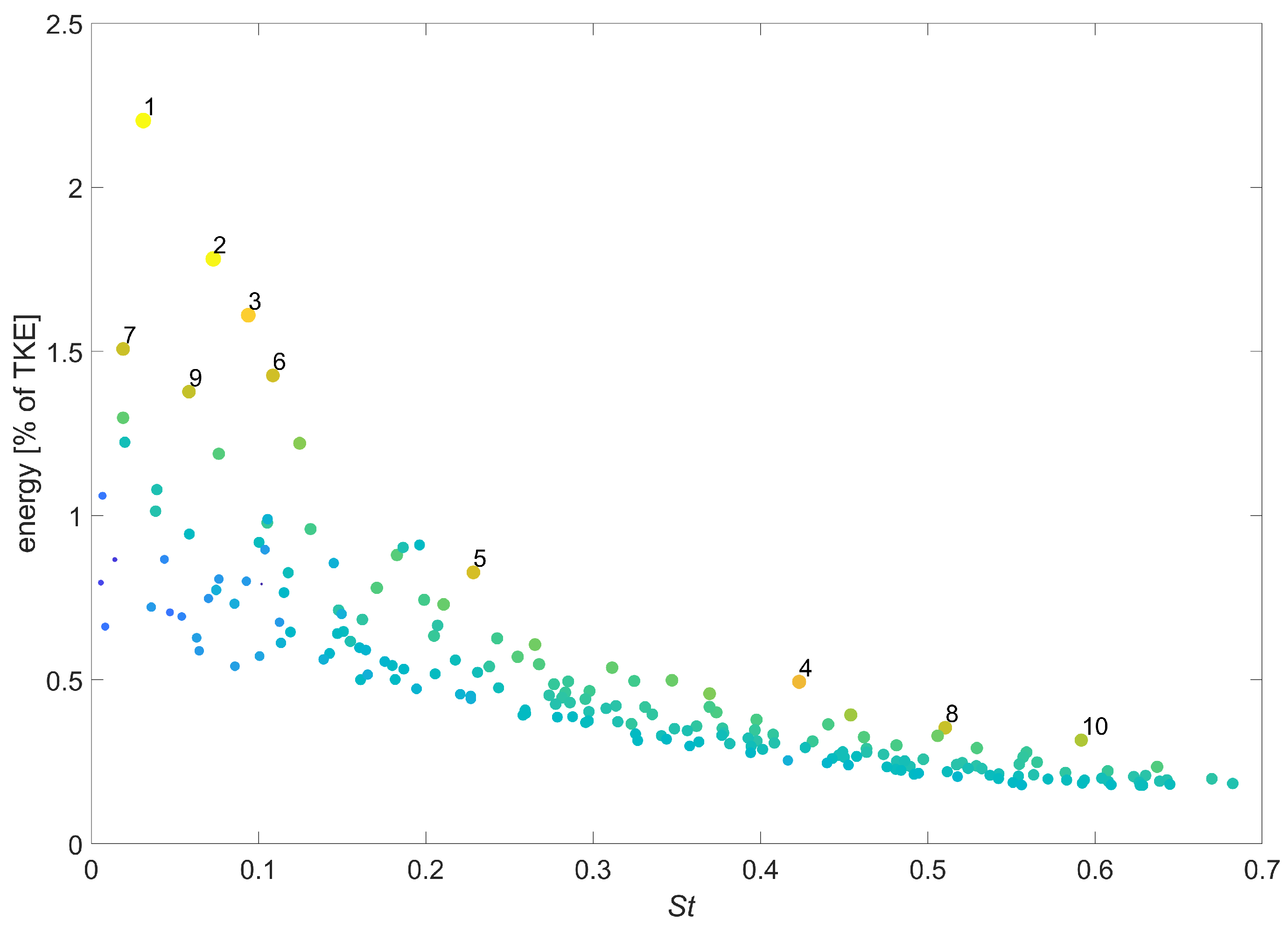
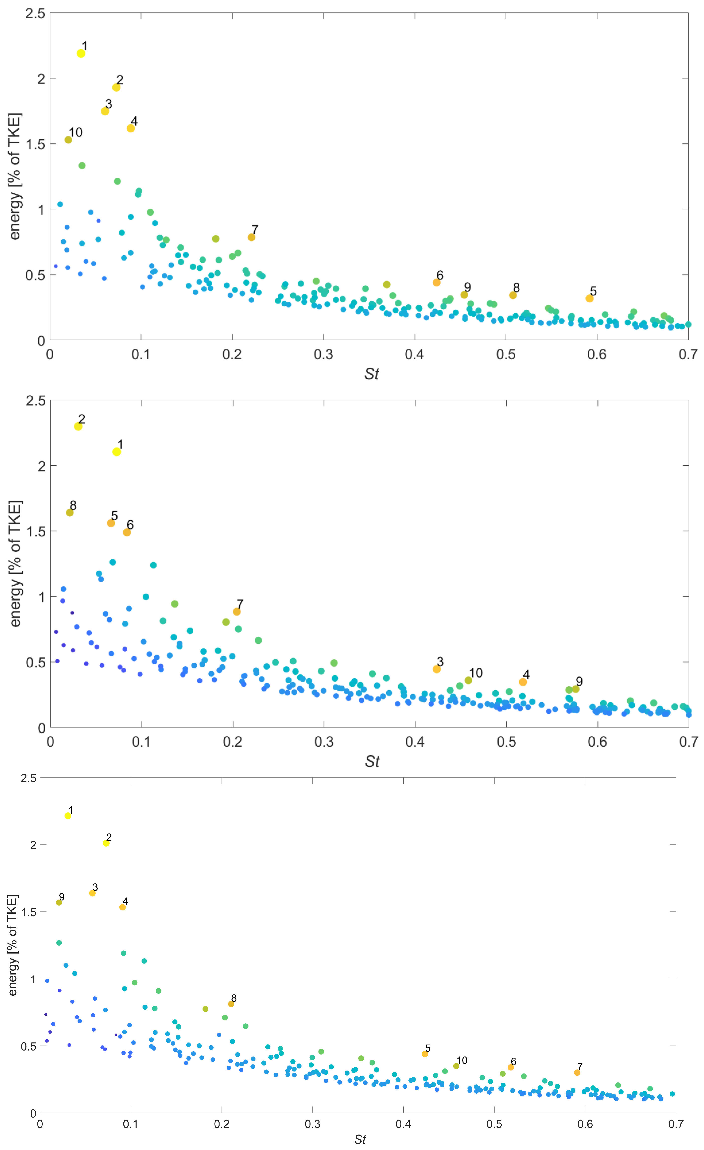
| 3D-Data | YZ-Plane | ||||
|---|---|---|---|---|---|
| Strouhal | Energy | Harmonic Correlation | Strouhal | Energy | Harmonic Correlation |
| 0.0311 | 2.20 | 0.914 | 0.0307 | 2.21 | 0.969 |
| 0.0729 | 1.78 | 0.900 | 0.0729 | 2.01 | 0.966 |
| 0.0938 | 1.61 | 0.810 | 0.0577 | 1.64 | 0.876 |
| 0.4231 | 0.49 | 0.744 | 0.0909 | 1.53 | 0.862 |
| 0.2283 | 0.83 | 0.706 | 0.4236 | 0.44 | 0.854 |
| 0.1085 | 1.43 | 0.701 | 0.5181 | 0.34 | 0.849 |
| 0.0190 | 1.51 | 0.694 | 0.5911 | 0.30 | 0.825 |
| 0.5104 | 0.35 | 0.691 | 0.2103 | 0.81 | 0.803 |
| 0.0584 | 1.38 | 0.685 | 0.0209 | 1.57 | 0.768 |
| 0.5917 | 0.32 | 0.661 | 0.4579 | 0.35 | 0.756 |
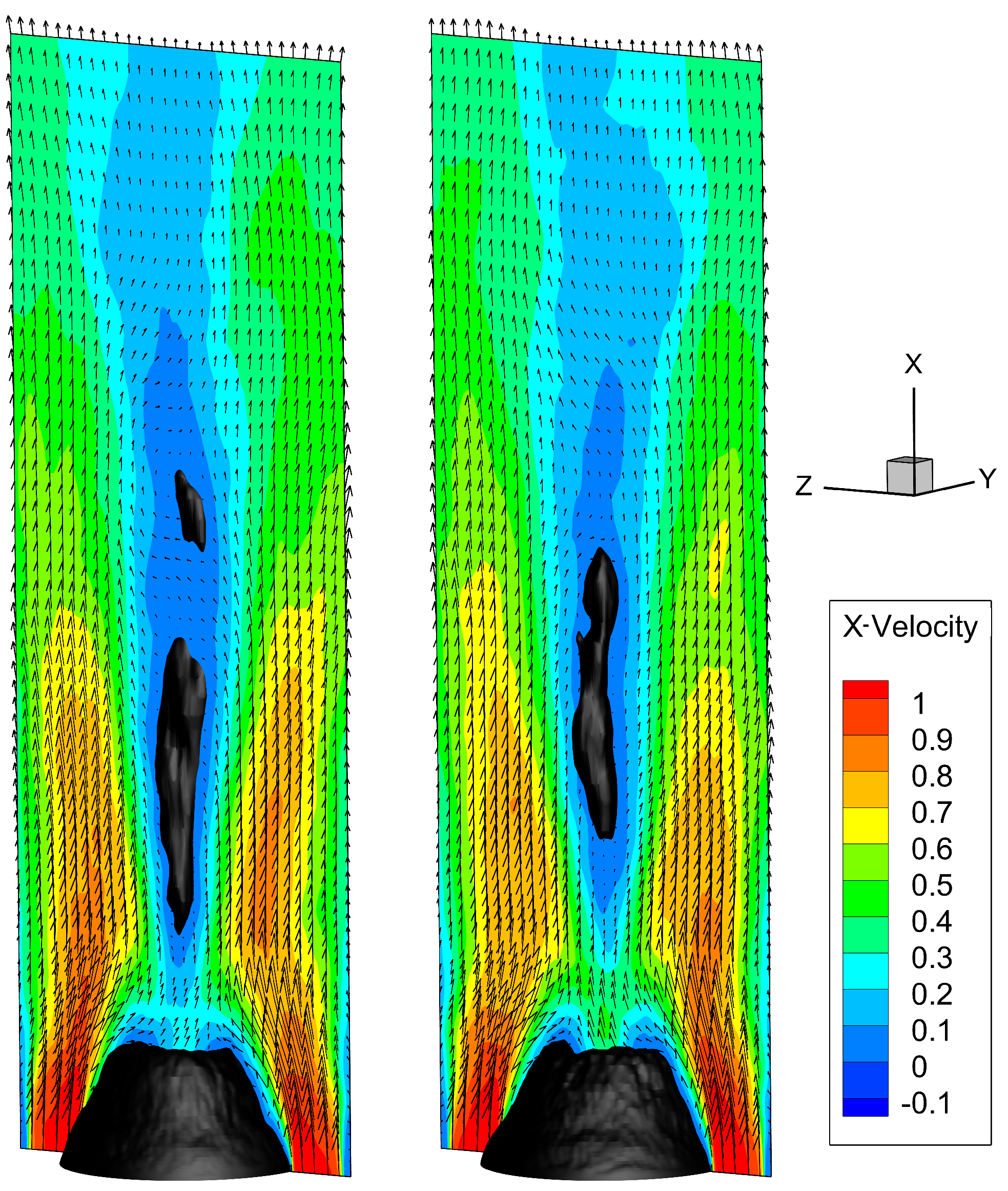
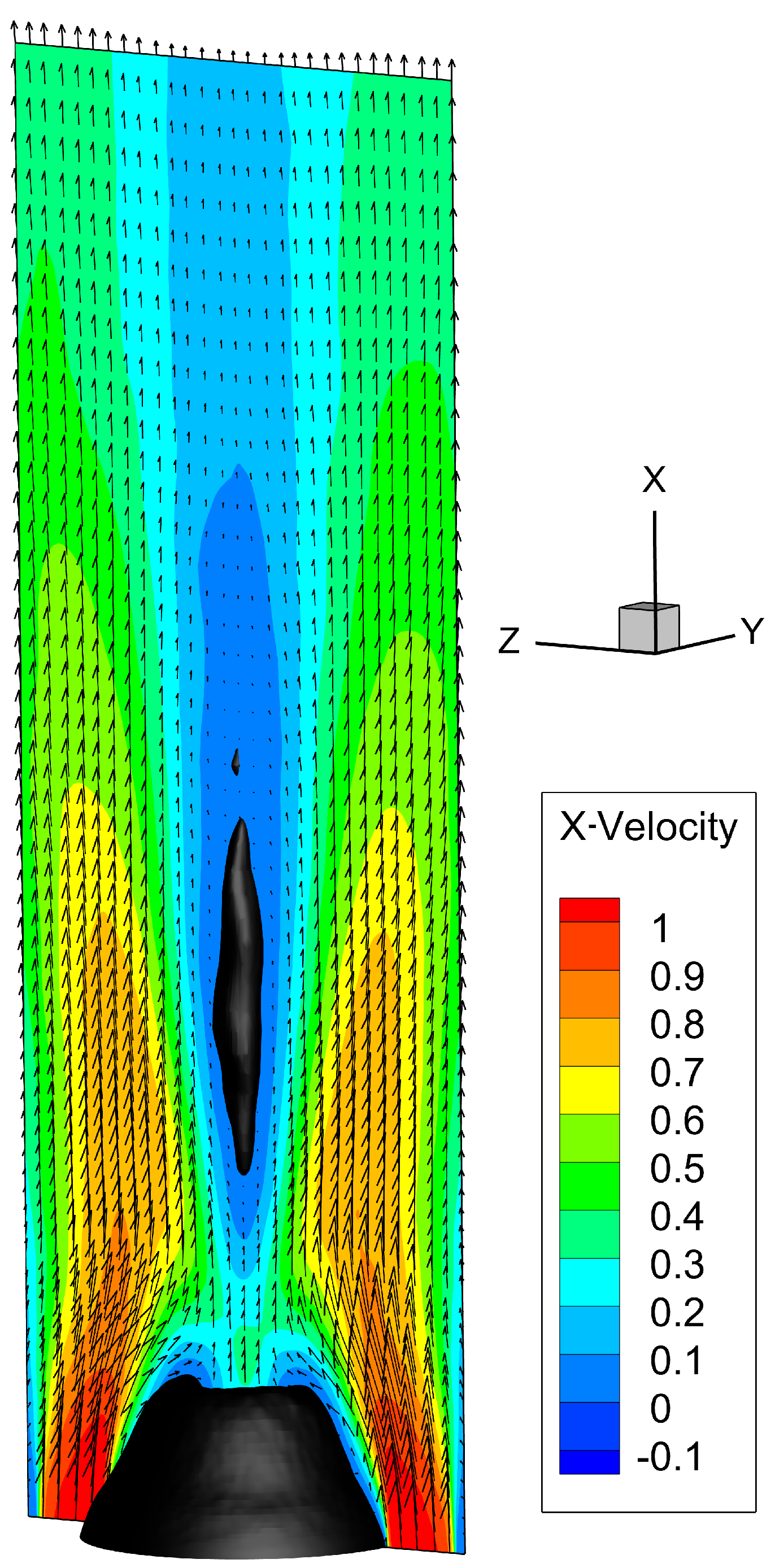
| Processing Time (s) | Strouhal Number–Single Helix | Strouhal Number–Double Helix | |
|---|---|---|---|
| 2D ROM—Y plane | 13 | 0.221 | 0.508 |
| 2D ROM—Z plane | 0.204 | 0.518 | |
| 2D ROM—YZ plane | 26 | 0.210 | 0.518 |
| 3D ROM | 1775 | 0.228 | 0.510 |
Publisher’s Note: MDPI stays neutral with regard to jurisdictional claims in published maps and institutional affiliations. |
© 2022 by the authors. Licensee MDPI, Basel, Switzerland. This article is an open access article distributed under the terms and conditions of the Creative Commons Attribution (CC BY) license (https://creativecommons.org/licenses/by/4.0/).
Share and Cite
Holemans, T.; Yang, Z.; Vanierschot, M. Efficient Reduced Order Modeling of Large Data Sets Obtained from CFD Simulations. Fluids 2022, 7, 110. https://doi.org/10.3390/fluids7030110
Holemans T, Yang Z, Vanierschot M. Efficient Reduced Order Modeling of Large Data Sets Obtained from CFD Simulations. Fluids. 2022; 7(3):110. https://doi.org/10.3390/fluids7030110
Chicago/Turabian StyleHolemans, Thomas, Zhu Yang, and Maarten Vanierschot. 2022. "Efficient Reduced Order Modeling of Large Data Sets Obtained from CFD Simulations" Fluids 7, no. 3: 110. https://doi.org/10.3390/fluids7030110
APA StyleHolemans, T., Yang, Z., & Vanierschot, M. (2022). Efficient Reduced Order Modeling of Large Data Sets Obtained from CFD Simulations. Fluids, 7(3), 110. https://doi.org/10.3390/fluids7030110