Note on the Bulk Estimate of the Energy Dissipation Rate in the Oceanic Bottom Boundary Layer

Abstract

The dissipation of the kinetic energy (KE) associated with oceanic flows is believed to occur primarily in the oceanic bottom boundary layer (BBL), where bottom drag converts the KE from mean flows to heat loss through irreversible mixing at molecular scales. Due to the practical difficulties associated with direct observations on small-scale turbulence close to the seafloor, most up-to-date estimates on bottom drag rely on a simple bulk formula ($C_d{U}^3$) proposed by G.I. Taylor that relates the integrated BBL dissipation rate to a drag coefficient ($C_d$) as well as a flow magnitude outside of the BBL (U). Using output from several turbulence-resolving direct numerical simulations, it is shown that the true BBL-integrated dissipation rate is approximately 90% of that estimated using the classic bulk formula, applied here to the simplest scenario where a mean flow is present over a flat and hydrodynamically smooth bottom. It is further argued that Taylor’s formula only provides an upper bound estimate and should be applied with caution in the future quantification of BBL dissipation; the performance of the bulk formula depends on the distribution of velocity and shear stress near the bottom, which, in the real ocean, could be disrupted by bottom roughness.

1. Introduction

Large-scale ocean currents are primarily powered by atmospheric winds and astronomical tidal forces at rates well quantified through satellite observations [1]. The work done by winds acting on the large-scale ocean currents inputs kinetic energy (KE) at a rate of around 0.8–0.9 TW [1,2,3], but the subsequent fate of this KE flux remains elusive. A large fraction of the KE input is converted into a vigorous mesoscale eddy field through the baroclinic instabilities of the large-scale currents and accounts for approximately 90% of the total ocean KE [4]. It is a topic of active research how the mesoscale energy is eventually dissipated at molecular scales. A prime candidate is thought to be bottom drag, i.e., the generation of vigorous turbulence along the ocean seafloor, which effectively transfers energy to smaller dissipative scales. Problematically, attempts to estimate the energy dissipated through bottom drag have resulted in widely differing estimates [1,5,6,7].

Bottom drag is experienced by oceanic flows above the seafloor, where a stress develops that brings the flow to zero. This occurs in a thin bottom boundary layer (BBL) characterized by enhanced shear and turbulence. The bottom stress ${\tau }_b$ is given by:

$${\tau }_b\equiv {\rho }_0\nu {\left.\frac{\partial u}{\partial z}\right|}_{z=0},$$

(1)

where z is the vertical coordinate relative to the bottom, $\nu$ is the molecular viscosity, ${\rho }_0$ is a reference density (seawater density varies by no more than a few percent across the global ocean) and $u\left(z\right)$ is the velocity component parallel to the seafloor. The bottom friction is often expressed in terms of a friction velocity defined as

$$u_{\tau }\equiv \sqrt{{\tau }_b/{\rho }_0}.$$

(2)

In the real turbulent ocean, it is difficult to estimate the bottom stress using Formula (1), because it requires detailed knowledge of rapid shear fluctuations very close to the boundary. Instead, the bottom stress is typically calculated using an empirical quadratic drag law

$${\tau }_b={\rho }_0{C}_d{U}^2,$$

(3)

where $C_d$ is a drag coefficient and U is the magnitude of the mean flow above the BBL, the so-called “far-field” velocity. This formula relates the bottom stress to dynamic pressure (proportional to $U^2$) associated with the mean flow [8].

Taylor went a step further and proposed to estimate the KE dissipation within the BBL, $\mathcal{D}$, as the product of the bottom stress and the “far-field” velocity [9]:

$$\mathcal{D}\equiv {\int }_{\mathrm{BBL}}ϵ\left(z\right)dz\simeq \frac{{\tau }_b}{{\rho }_0}U=C_d{U}^3,$$

(4)

where $ϵ$ is the point-wise KE dissipation rate defined as

$$ϵ=\frac{\nu }{2}{S}_{ij}{S}_{ij},$$

(5)

and $S_{ij}=\partial u_i/\partial x_j+\partial u_j/\partial x_i$ is the rate of strain tensor. Taylor used this bulk formula to estimate the dissipation experienced by barotropic tides over continental shelves and set U to be the barotropic tidal velocity [9]. This bulk formula was later used to estimate the dissipation of sub-inertial flows in the global ocean and returned values anywhere between 0.2 and 0.83 TW [1,5,6,7]. Based on these estimates, bottom drag could be a dominant sink of the 0.8–0.9 TW KE input by winds or a second-order process.

In this study, we will take a closer look at the reasoning and assumptions behind Taylor’s KE dissipation formula (Equation (4)) and compare this bulk estimate with explicitly diagnosed KE dissipation rates from turbulence-resolving direct numerical simulations (DNS). We find that although the formula slightly overestimates the integrated BBL energy dissipation rate, it provides satisfying bulk estimates in idealized numerical simulations of flows over a smooth flat bottom. The difference between the two depends on the distribution of velocity and shear stress close to the seafloor, which implies a possibly larger discrepancy when the inner layer BBL structure is disrupted by bottom roughness in the real ocean. The DNS data are described in Section 2. In Section 3, we illustrate how the vertical profiles of stress and velocity shear determine the performance of Taylor’s formula. Our hypothesis is confirmed by computing the vertical profiles of shear, stress and KE dissipation from the DNS in Section 4. In Section 5, we derive a heuristic formula that predicts the performance of Taylor’s formula at a realistically large frictional Reynolds number Re${}_{\tau }$. The implications of our work for oceanographic estimates of energy dissipation in the BBL are discussed in Section 6.

2. Data and Methods

The data analyzed in this study come from four DNS of a mean flow over a smooth flat bottom—two without rotation [10] and two with rotation [11]—the so-called bottom Ekman layer. The simulations are characterized using frictional Reynolds number Re${}_{\tau }=u_{\tau }\delta /\nu =\delta /{\delta }_{\nu }$, where ${\delta }_{\nu }=\nu /u_{\tau }$ is the viscous length scale. The bottom boundary condition is no-slip in all simulations, and the top boundary condition is a prescribed velocity equal to the free-stream flow. The diagnostics are obtained by horizontally averaging over the model domain once the solutions have achieved a statistically steady state. More details about the simulations are given in

Table 1. Summary of the DNS experiments. Note that the drag coefficient $C_d$ in each run can be obtained using $C_d={(u_{\tau }/U)}^2$ considering ${\tau }_b={\rho }_0{C}_d{U}^2$ and $u_{\tau }\equiv \sqrt{{\tau }_b/{\rho }_0}$.

No.	Re${}_{\mathit{\tau }}$(Re${}_{\mathit{f}}$)	${\mathit{u}}_{\mathit{\tau }}/\mathit{U}$	Type	$\mathcal{D}$/${\mathit{C}}_{\mathit{d}}{\mathit{U}}^3$
1	830	4.08$\times {10}^{-2}$	non-rotating	0.8614
2	1271	3.85$\times {10}^{-2}$	non-rotating	0.8638
3	943	5.61$\times {10}^{-2}$	rotating	0.9082
4	1765	5.21$\times {10}^{-2}$	rotating	0.9178

.

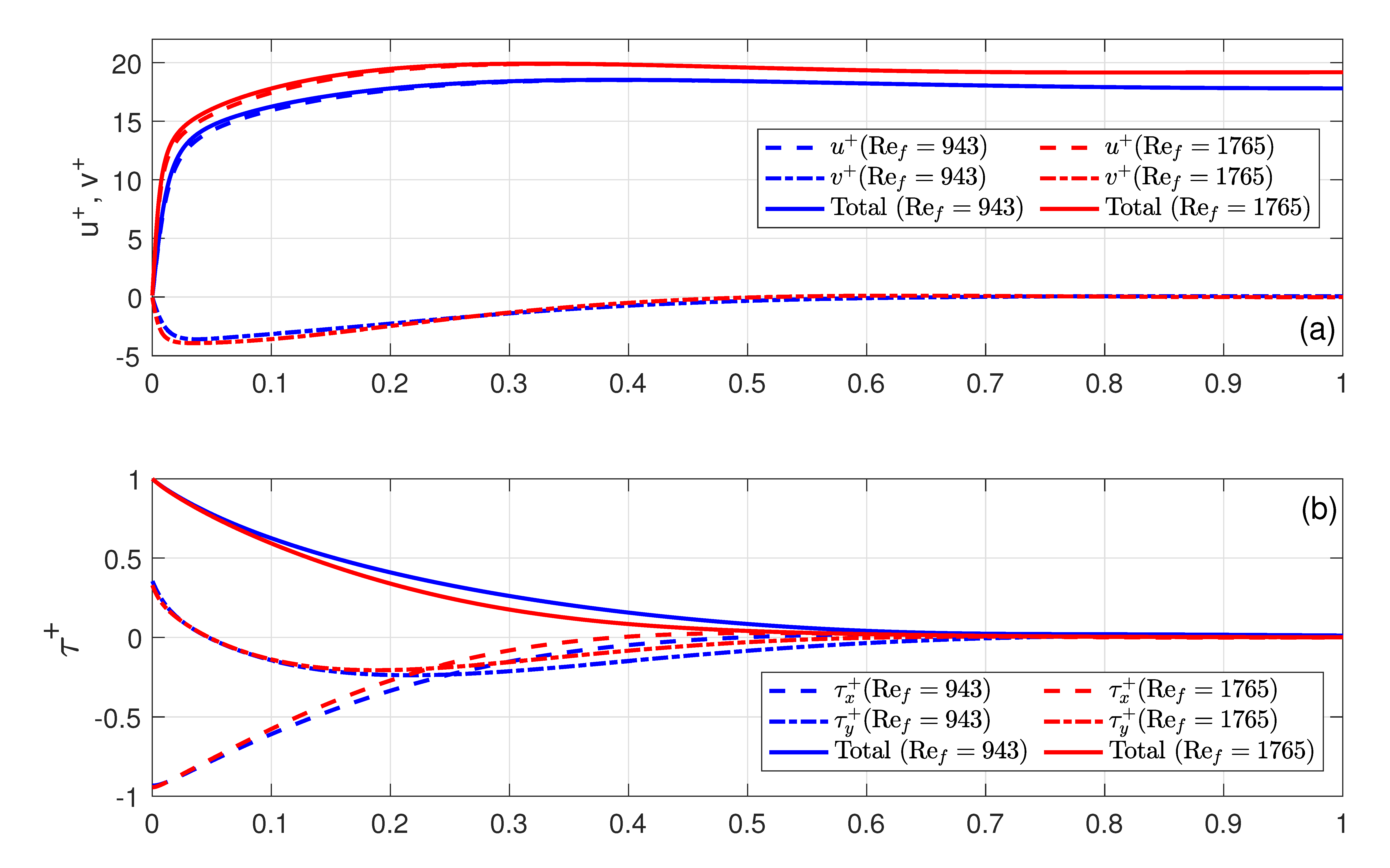
For the rest of the paper, we will use $\delta$ as the boundary layer thickness for both setups. In the non-rotating case, $\delta$ denotes the distance across the boundary layer from the bottom wall to a point where the flow velocity has essentially reached the ’free-stream’ velocity (99% of U); in the rotating case, we adopt the common Ekman layer scaling, $\delta =u_{\tau }/f$, where f is the Coriolis frequency. Considering the difference in the definition of boundary layer thickness, we will use Re${}_{\tau }=u_{\tau }\delta /\nu$ for the non-rotating BBL and Re${}_f=u_{\tau }^2/f\nu$ for the rotating BBL, where the boundary layer thickness is replaced with the Ekman layer scaling. Note, however, that these two Reynolds numbers are comparable, as will be shown in Section 4. Finally, all the diagnostics are non-dimensionalized by the appropriate combination of frictional variables $\nu$ and $u_{\tau }$; for instance, the non-dimensional dissipation rate is given by ${ϵ}^{+}=ϵ\nu /u_{\tau }^4$.

3. The Impact of the Vertical Shear Profile on BBL Dissipation

We start by computing the integrated BBL dissipation rate in a non-rotating BBL for idealized vertical profiles of velocity and shear stress in order to illustrate their impacts on the bulk estimates. We assume a horizontal flow u above a solid bottom, and that all variables are independent of horizontal position and vary only with distance above the bottom. The total energy dissipation rate (per unit mass) within the BBL can simply be calculated as the vertical integral of the product of u and the vertical gradient of total shear stress $\tau$:

$$\begin{array}{c}\hfill \mathcal{D}=-{\int }_0^{\delta }u\frac{\partial \tau }{\partial z}dz={\int }_0^{\delta }\tau \frac{\partial u}{\partial z}dz={\int }_0^{\delta }{C}_d{U}^2\left(\frac{\delta -z}{\delta }\right)\frac{\partial u}{\partial z}dz.\end{array}$$

(6)

where $\tau$ includes both viscous and Reynolds stresses and we integrated by parts using the fact that the velocity u vanishes at $z=0$ and the shear stress vanishes at $z=\delta$. The shear stress has been approximated as a linearly decaying profile in z [12]:

$$\tau \left(z\right)={\tau }_b\left(\frac{\delta -z}{\delta }\right).$$

(7)

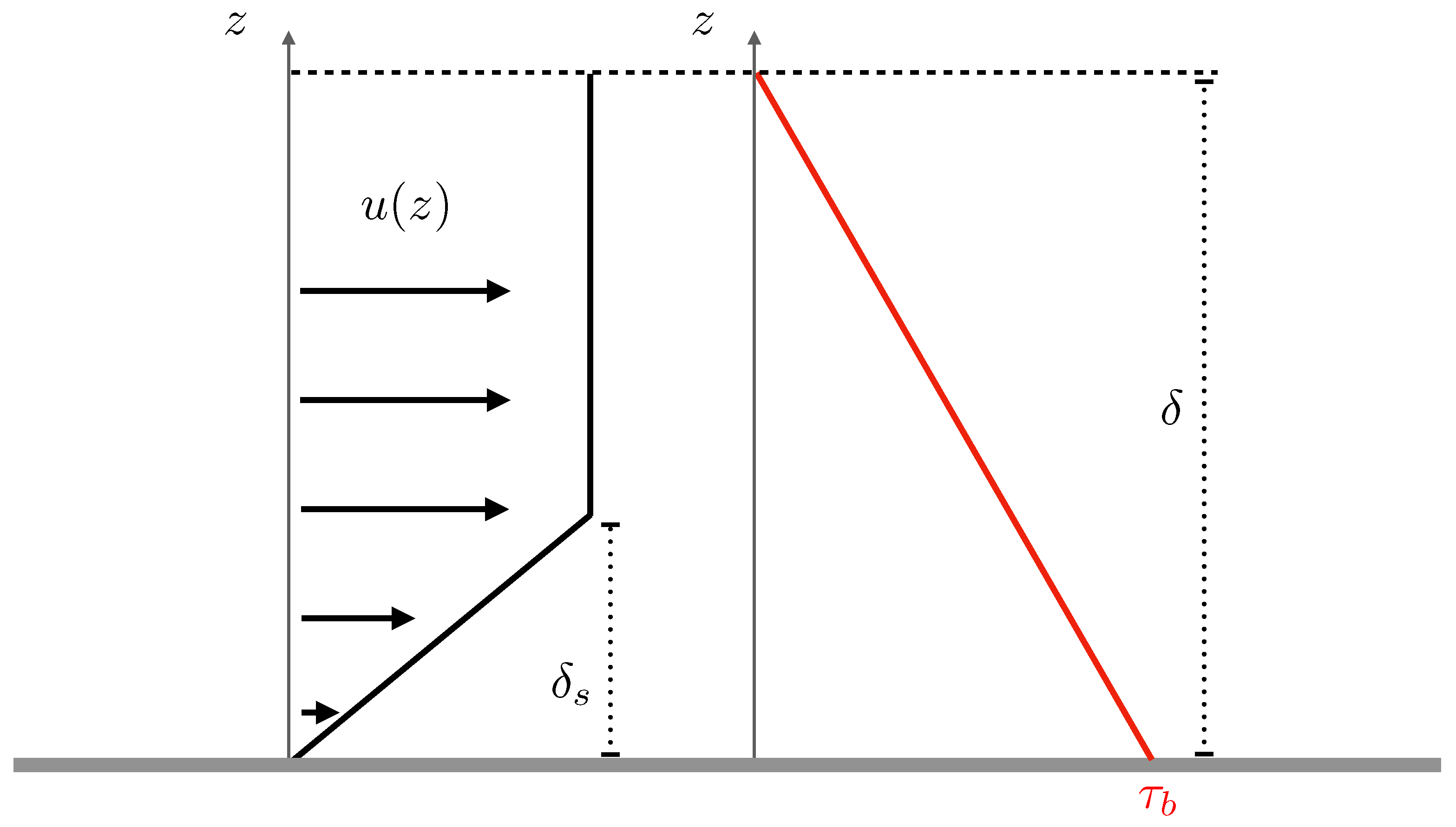
Taylor’s formula follows from Equation (6) only if the velocity profile u is uniform and equal to the far-field velocity U, but this is not the case in reality. Instead, the velocity profile decays to zero within the BBL due to the no-slip bottom boundary condition. If we assume, for simplicity, that the velocity profile is linear in z up to $z={\delta }_s$, where it reaches the far-field velocity U, and remains constant above (Figure 1) (in other words, we only consider the large velocity shear confined in a thin layer of thickness ${\delta }_s$ near the bottom and we ignore any negligibly small changes above), the integral in Equation (6) can be rewritten as:

$$\mathcal{D}={\int }_0^{{\delta }_s}{C}_d{U}^2\left(\frac{\delta -z}{\delta }\right)\frac{U}{{\delta }_s}dz=C_d{U}^3(1-\frac{1}{2}\frac{{\delta }_s}{\delta }).$$

(8)

For this admittedly idealized piece-wise linear velocity profile, Taylor’s formula is recovered only in the limit where the velocity shear is confined to a layer much thinner than the BBL (${\delta }_s\ll \delta$).

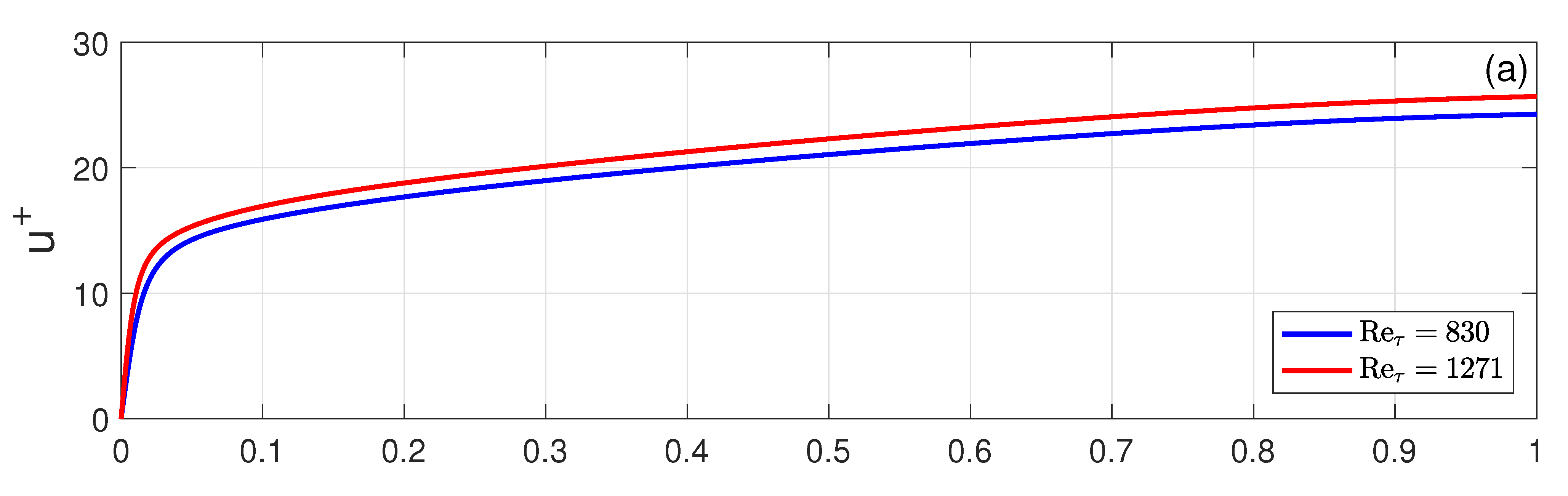
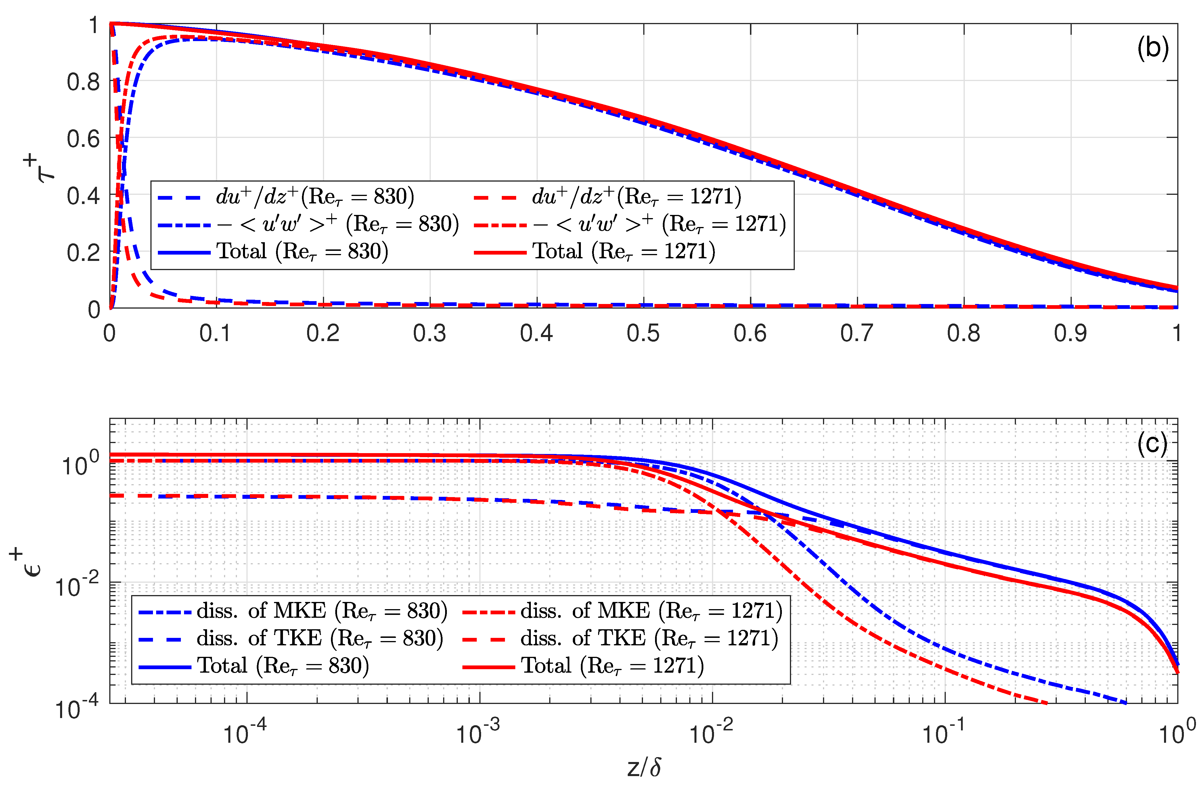
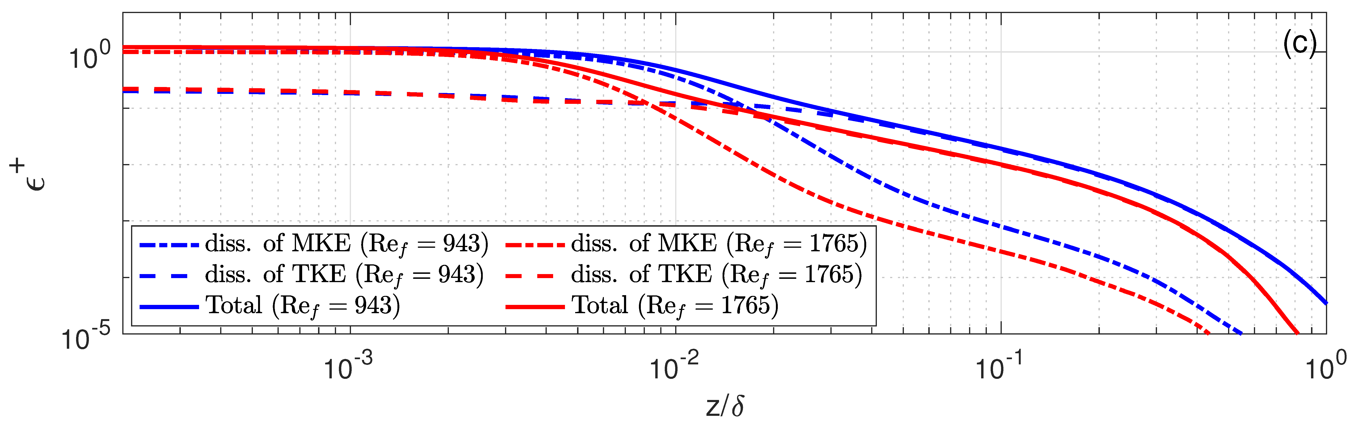
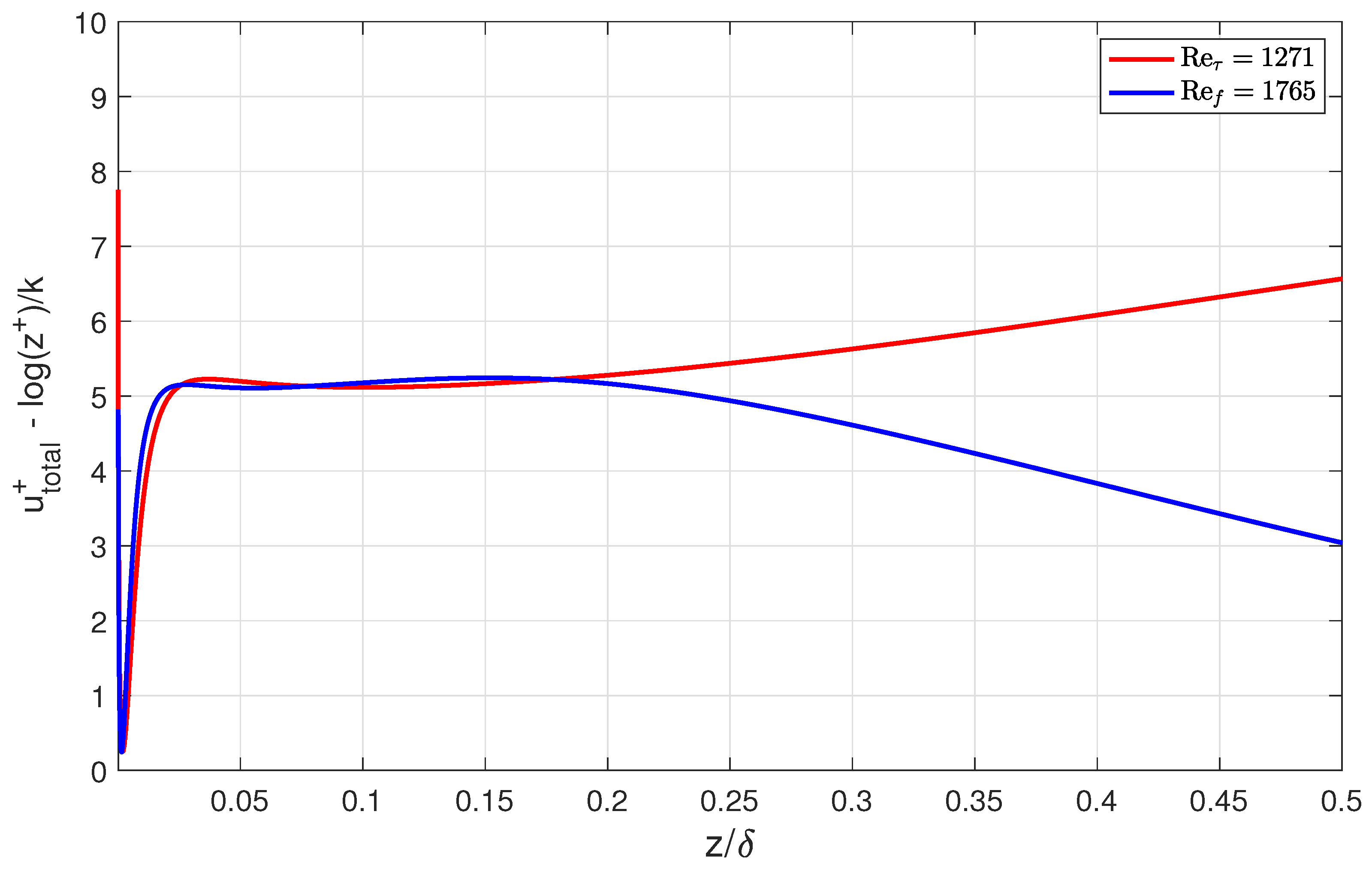
The vertical profiles of velocity and shear stress in the DNS of non-rotating BBL are shown in Figure 2 for two different Re${}_{\tau }$. Supporting the main idealization associated with our heuristic model introduced above, two observations can be made: (i) the largest velocity shear is confined within a thin layer near the bottom (Figure 2a and dashed lines in Figure 2b); (ii) the decay of the total shear stress follows a rather linear profile (solid lines in Figure 2b). As Re${}_{\tau }$ increases, the layer accounting for the large velocity shear becomes thinner and closer to the wall. While the shear layer thickness is always thinner than $\delta$, and progressively more so for increasing Re${}_{\tau }$, it clearly differs from the limit where the shear layer is infinitesimally thin, as assumed in Taylor’s formula. We will evaluate the impact of this discrepancy in the next section.

4. Vertical Structures of the BBL

4.1. Non-Rotating BBL

Along with the thin layer containing the large velocity shear is enhanced viscous stress and the associated dissipation of mean kinetic energy (MKE) within the BBL (Figure 2b,c). The viscous stress is dominant for $z/\delta ⪅0.02$ due to both the enhanced velocity shear and the damping of Reynolds stress in the presence of the solid bottom. Again, the distribution of the total shear stress provides support for the linear approximation made in the idealized heuristic model in the last section. As Re${}_{\tau }$ increases, both the viscous and Reynolds stress become closer to the bottom, but the structure of the total shear stress remains relatively unchanged (Figure 2b).

The dissipation of MKE acts as an additional route to energy dissipation and has been typically thought to be negligible in turbulent flows away from boundaries with moderate to large Reynolds numbers. It cannot be ignored, however, in the BBL, where the velocity shear is confined close to the bottom. In this case, MKE dissipation contributes around 40% of the total energy dissipation rate. On the other hand, the dissipation of turbulent kinetic energy (TKE) becomes dominant beyond $z/\delta =0.02$ and remains so all the way to the top of the BBL. The transition point between the dissipation of MKE and TKE becomes closer to the bottom with larger Re${}_{\tau }$.

From the simulations, we can calculate the ratios between the true KE dissipation rate (using Equation (5)) integrated across the BBL and those estimated with Taylor’s bulk formula: ${\tau }_b$ can be directly obtained from Equation (1) in each run, as with the drag coefficient $C_d$ and friction velocity $u_{\tau }$ (Table 1). The ratio of the two can be written as:

$$\frac{\mathcal{D}}{C_d{U}^3}=\frac{u_{\tau }^3{\int }_{\mathrm{BBL}}{ϵ}^{+}\left(z^{+}\right)d{z}^{+}}{u_{\tau }^{2}U}=\frac{u_{\tau }}{U}{\int }_{\mathrm{BBL}}{ϵ}^{+}\left(z^{+}\right)d{z}^{+}.$$

(9)

The calculated $\mathcal{D}/C_d{U}^3$ ratios for the two simulations of non-rotating BBL are 86.1% and 86.4%, respectively (Table 1). These ratios imply that the ${\delta }_s/\delta$ ratio in Equation (8) is around 0.28; this depth of shear layer ${\delta }_s$ roughly corresponds to ${ϵ}^{+}={10}^{-2}$ (Figure 2c). We will examine the performance of Taylor’s formula in the rotating BBL next.

4.2. Rotating BBL

When rotation is introduced, the simulated velocity profiles show a spiral structure as they approach the far-field mean flow (Figure 3a). One noticeable difference from the non-rotating BBL is the more bottom-confined or concave profiles for both velocity shear and shear stress (Figure 3a,b), compared with the more linear shear profile in the non-rotating BBL. The rest of the structures remain similar in the BBL with or without rotation.

In the two simulations of rotating BBL, the true integrated KE dissipation rate is 90.8% and 91.8% of those estimated using Taylor’s bulk formula (using Equation (9)), higher than those for the non-rotating BBL for comparable Re${}_f$. This better performance could be explained by the more bottom-confined velocity shear and shear stress profiles.

In summary, Taylor’s bulk formula provides reasonable first-order estimates for the true integrated dissipation rate. In fact, $\mathcal{D}$/$C_d{U}^3\approx 0.9$, which is the equivalent of ${\delta }_s/\delta \approx 0.2$, is consistent with the observations that the log-layer, where the largest velocity shear and shear stress reside, roughly occupies 20% of the BBL thickness for both the rotating and non-rotating BBLs (Figure 4). This 20% has also been shown to hold for natural turbulent flows with much larger Re${}_{\tau }$ [13], which implies that Taylor’s formula could provide a reasonable integrated dissipation estimate in the real ocean, given that the log-layer structure remains intact.

5. An Empirical Formula for Large Re${}_{\tau }$

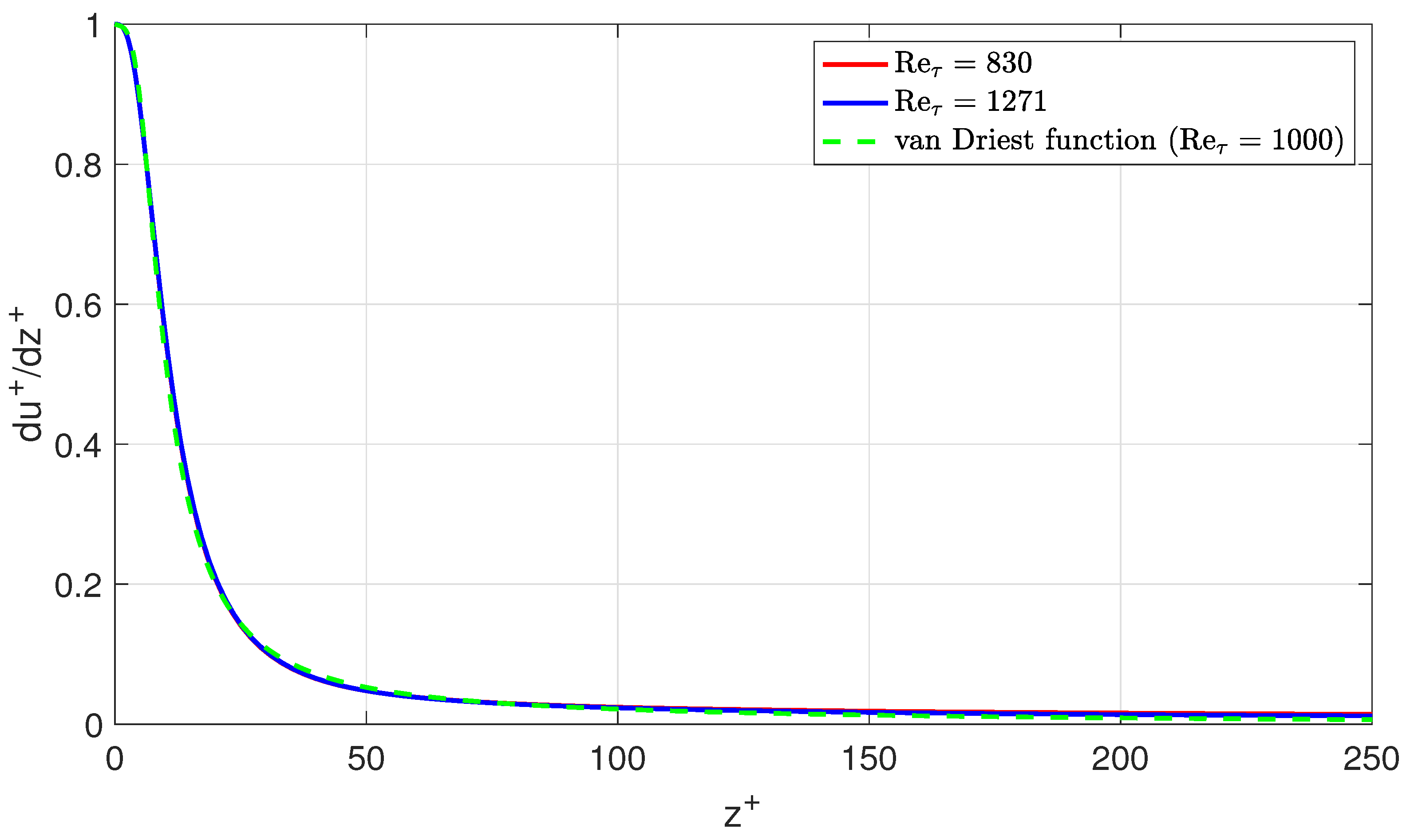
To improve on the prediction of the heuristic model and extend the findings to realistically large Re${}_{\tau }$ for real ocean applications, we repeat the analysis in Section 3 but with a more physical velocity profile derived by van Driest [14]. Note that the prediction is only performed for the non-rotating BBL since relevant analytical profiles for the rotating BBL structures are still lacking. The analytical shear profile is introduced based on mixing length arguments:

$$\frac{\partial u^{+}}{\partial z^{+}}=\frac{2(1-z^{+}/{\mathrm{Re}}_{\tau })}{1+{[1+4(1-z^{+}/{\mathrm{Re}}_{\tau }){\left(l_m^{+}\right)}^2]}^{1/2}}$$

(10)

where

$$l_m^{+}=k{z}^{+}[1-exp(-z^{+}/\zeta )]$$

(11)

is a mixing length that decreases rapidly close to the wall, representing the damping of the log-layer mixing length $k{z}^{+}$ due to the presence of the solid boundary. $k=0.41$ is the von Kármán constant and $\zeta$ is a constant with a typical value of 26. Figure 5 demonstrates that the analytical profile captures well the velocity shear from the numerical simulations.

Substituting van Driest’s analytical Formula (10) into the integral formula for the BBL dissipation given in Equation (6) and again assuming a linear decaying function for the total shear stress, we obtain:

$$\mathcal{D}=C_d{U}^2{u}_{\tau }{\int }_0^{{\mathrm{Re}}_{\tau }}\left(1-\frac{z^{+}}{{\mathrm{Re}}_{\tau }}\right)\frac{\partial u^{+}}{\partial z^{+}}\mathrm{d}{z}^{+}=\mathrm{I}\left({\mathrm{Re}}_{\tau }\right)\frac{u_{\tau }}{U}{C}_d{U}^3,$$

(12)

where I$\left({\mathrm{Re}}_{\tau }\right)$ is a growing function of Re${}_{\tau }$ given by the integral expression:

$$\mathrm{I}\left({\mathrm{Re}}_{\tau }\right)={\int }_0^{{\mathrm{Re}}_{\tau }}\frac{2{(1-z^{+}/{\mathrm{Re}}_{\tau })}^2}{1+{[1+4(1-z^{+}/{\mathrm{Re}}_{\tau }){\left(l_m^{+}\right)}^2]}^{1/2}}\mathrm{d}{z}^{+}.$$

(13)

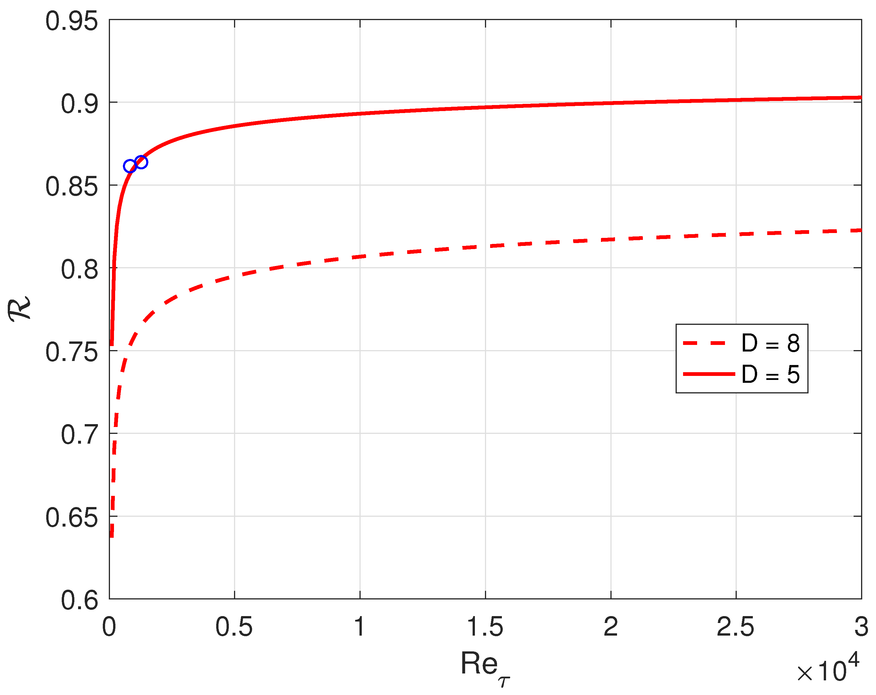
Finally, the ratio of the integrated BBL dissipation rate based on van Driest’s analytical expression and that proposed by Taylor is given by:

$$\mathcal{R}\equiv \frac{\mathcal{D}}{C_d{U}^3}=\mathrm{I}\left({\mathrm{Re}}_{\tau }\right)\frac{u_{\tau }}{U}.$$

(14)

Pope [12] showed that $U/u_{\tau }=k^{-1}ln\left({\mathrm{Re}}_{\tau }\right)+D$, where D is a constant that depends on the problem geometry. Thus, the ratio in Equation (14) can be expressed as a function of ${\mathrm{Re}}_{\tau }$ only:

$$\mathcal{R}\left({\mathrm{Re}}_{\tau }\right)=\frac{\mathrm{I}\left({\mathrm{Re}}_{\tau }\right)}{k^{-1}ln\left({\mathrm{Re}}_{\tau }\right)+D}.$$

(15)

The prediction of $\mathcal{R}\left({\mathrm{Re}}_{\tau }\right)$ to realistically large ${\mathrm{Re}}_{\tau }$ is shown in Figure 6 with two different choices of D. For our two non-rotating BBL simulations, D is found to be around 8 based on the $U/u_{\tau }$ ratios given in Table 1, but we need to adjust the D value to 5 when estimating the integrated dissipation rate to match the existing simulation results. This adjustment for higher-order statistics (i.e., dissipation) may be justified as a way to compensate for the idealizations introduced in the heuristic model, such as possible deviations from the assumed perfect linear profile of shear stress. While it is indeed the case that the ratio approaches one for infinite ${\mathrm{Re}}_{\tau }$, the convergence for larger ${\mathrm{Re}}_{\tau }$ becomes very slow and our non-rotating BBL results are very close to the “saturated” value of $\mathcal{R}=0.9$ (Figure 6). It is unclear whether the prediction for the rotating BBL follows a similar asymptotic trend; it is likely that the calculated $\mathcal{R}$ values for the rotating BBL presented here are already in the slow-converging regime considering that the velocity shear is more confined to the solid bottom compared with the non-rotating BBL at comparable Reynolds numbers. This will need to be addressed in future studies.

Formula (15) quantifies the amount by which Taylor’s formula overpredicts the integrated dissipation taking place over a flat BBL. To appreciate the oceanographic implications of this result, it is worth applying the formula to parameters typical of oceanic BBL: $C_d=1\times {10}^{-3}$, $U=0.15$ m/s, $\delta =10$ m and $\nu =1.5\times {10}^{-6}$ m${}^2$/s. With these values, Re${}_{\tau }=3\times {10}^4$ and the formula gives $\mathcal{R}=\frac{\mathcal{D}}{C_d{U}^3}=0.90$. The degree to which results based on flat walls may be used over the rugged ocean bottom will be discussed in the next section.

6. Conclusions and Discussion

Four DNS experiments were used to demonstrate that the KE dissipation rate in the BBL over a flat wall is less than predicted by the celebrated formula proposed by Taylor [9]: $\mathcal{D}\simeq C_d{U}^3$, where $C_d$ is a constant drag coefficient and U the "far-field" velocity above the BBL. Taylor’s estimate should be treated as an upper and singular limit of the true BBL-integrated KE dissipation rate. The discrepancy arises due to the assumption that the shear in the BBL is confined to an infinitesimally thin layer within the viscous sublayer in Taylor’s formula. It is shown that the shear actually extends far above the viscous sublayer to approximately 20% of the BBL thickness for even the largest frictional Reynolds numbers Re${}_{\tau }$ expected in natural flows. Taylor’s formula could thus be improved to be $\mathcal{D}\approx 0.9\times C_d{U}^3$ for a more accurate prediction. We note that this is a modest correction compared with the other uncertainties in real ocean applications. The local uncertainties associated with the drag coefficient $C_d$ and the identification of the far-field velocity U when using Taylor’s formula could introduce much larger errors in problems encountered in the real ocean. Nonetheless, we believe that the findings in this study will be helpful in future BBL dissipation estimates, especially in cases where $C_d$ and U are well measured or when their local variations can be ignored in large-scale BBL dissipation quantification.

Admittedly, Taylor’s formula provides a good first-order estimate for the integrated BBL dissipation rate. However, the evaluation performed in this note only applies to a smooth bottom where the viscous and log-layers are intact. The ocean seafloor is far from flat. Corrugations on scales smaller than the BBL thickness, typical of the ocean seafloor, could modify or even destroy the inner layer structures [15]. The small roughness can be accounted for by introducing a roughness parameter that quantifies the characteristic height of the corrugations, $z_o$. This results in a modification of the log-layer away from the bottom: $u\left(z\right)=\frac{u_{\tau }}{\kappa }log\frac{z}{z_o}$, e.g., [12,16]. It remains to be studied whether the disrupted viscous sublayer and the modified log-layer structure could have an impact on the energy dissipation estimate. Moreover, the log-layer could be completely destroyed when the roughness is large. A common parameter to consider here is the blockage ratio $\delta /k$, where k is the roughness height. This non-dimensional parameter measures the direct effect of the roughness on the log-layer, where most of the mean shear is concentrated. Previous studies have shown that $\delta /k$ has to be at least 40 for a general log-layer structure to hold [15]. This suggests that Taylor’s formula could fail over rough seafloors where the velocity shear is no longer concentrated close to the wall. Detailed velocity measurements near the seabed are very sparse and the existence of log-layer structures has only been reported over a few locations over the continental shelf, e.g., [17,18,19]; more observations are needed to assess the applicability of Taylor’s formula in the global ocean over more complex topography.

The DNS experiments presented here do not include stratification. This may not be the most problematic simplification of our work, because stratification is expected to be quite weak in oceanic BBL. Stratification is indeed very weak in the inner layer close to the seafloor due to enhanced mixing, e.g., [20,21]. Stratification may, however, be strong enough in the outer layer to suppress turbulent overturns larger than the Ozmidov scale $L_o={(ϵ/N^3)}^{1/2}$ (N being the Brunt–Väisälä frequency) and lead to a modification of the shear profile [18,19]. However, we showed that the bulk of the KE dissipation occurs in the log-layer, and not in the outer layer, where the distance to the bottom is the dominant limit on the eddy overturn size rather than the Ozimdov scale. Thus, we expect the influence of stratification on the integrated dissipation rate to be small. In real ocean applications, however, stratification may pose problems in identifying the far-field flow U, especially when over a sloping bottom [22,23,24,25].

In addition to small-scale roughness, BBL dissipation can be modified by the presence of large-scale slopes, such as along the flanks of ridges and seamounts [26,27,28], detachment of BBL at large Froude numbers, e.g., [29], and the development of a whole gamut of hydrodynamic subemsoscale instabilities and hydraulic jumps, e.g., [30,31]. Clearly, a full quantitative picture of BBL dissipation in the ocean remains far from complete. Our work has only shown that Taylor’s formula should be used with caution and treated as an upper limit of the integrated BBL dissipation rate in the case of a mean flow over the seafloor. Future examinations are needed to account for seafloor roughness and more realistic velocity and stress profiles before applying Taylor’s formula in global energy dissipation studies.

References

1. Wunsch, C.; Ferrari, R. Vertical mixing, energy, and the general circulation of the oceans. Annu. Rev. Fluid Mech. 2004, 36, 281–314. [Google Scholar] [CrossRef] [Green Version]
2. Wunsch, C. The work done by the wind on the oceanic general circulation. J. Phys. Oceanogr. 1998, 28, 2332–2340. [Google Scholar] [CrossRef]
3. Scott, R.B.; Xu, Y. An update on the wind power input to the surface geostrophic flow of the World Ocean. Deep. Sea Res. Part Oceanogr. Res. Pap. 2009, 56, 295–304. [Google Scholar] [CrossRef]
4. Ferrari, R.; Wunsch, C. Ocean circulation kinetic energy: Reservoirs, sources, and sinks. Annu. Rev. Fluid Mech. 2009, 41, 253–282. [Google Scholar] [CrossRef] [Green Version]
5. Sen, A.; Scott, R.B.; Arbic, B.K. Global energy dissipation rate of deep-ocean low-frequency flows by quadratic bottom boundary layer drag: Computations from current-meter data. Geophys. Res. Lett. 2008, 35. [Google Scholar] [CrossRef]
6. Arbic, B.K.; Shriver, J.F.; Hogan, P.J.; Hurlburt, H.E.; McClean, J.L.; Metzger, E.J.; Scott, R.B.; Sen, A.; Smedstad, O.M.; Wallcraft, A.J. Estimates of bottom flows and bottom boundary layer dissipation of the oceanic general circulation from global high-resolution models. J. Geophys. Res. Ocean. 2009, 114. [Google Scholar] [CrossRef]
7. Wright, C.J.; Scott, R.B.; Furnival, D.; Ailliot, P.; Vermet, F. Global observations of ocean-bottom subinertial current dissipation. J. Phys. Oceanogr. 2013, 43, 402–417. [Google Scholar] [CrossRef] [Green Version]
8. Tritton, D.J. Physical Fluid Dynamics; Springer Science & Business Media: Berlin/Heidelberg, Germany, 2012. [Google Scholar]
9. Taylor, G.I. I. Tidal friction in the Irish Sea. Philos. Trans. R. Soc. Lond. Ser. Contain. Pap. Math. Phys. Character 1920, 220, 1–33. [Google Scholar]
10. Schlatter, P.; Örlü, R. Assessment of direct numerical simulation data of turbulent boundary layers. J. Fluid Mech. 2010, 659, 116–126. [Google Scholar] [CrossRef]
11. Miyashita, K.; Iwamoto, K.; Kawamura, H. Direct numerical simulation of the neutrally stratified turbulent Ekman boundary layer. J. Earth Simulator 2006, 6, 3–15. [Google Scholar]
12. Pope, S.B. Turbulent Flows; Cambridge University Press: Cambridge, UK, 2001. [Google Scholar]
13. Marusic, I.; Monty, J.P.; Hultmark, M.; Smits, A.J. On the logarithmic region in wall turbulence. J. Fluid Mech. 2013, 716. [Google Scholar] [CrossRef] [Green Version]
14. Van Driest, E.R. On turbulent flow near a wall. J. Aeronaut. Sci. 1956, 23, 1007–1011. [Google Scholar] [CrossRef]
15. Jiménez, J. Turbulent flows over rough walls. Annu. Rev. Fluid Mech. 2004, 36, 173–196. [Google Scholar] [CrossRef]
16. Tennekes, H.; Lumley, J.L. A first Course in Turbulence; MIT Press: Cambridge, MA, USA, 2018. [Google Scholar]
17. Caldwell, D.; Chriss, T. The viscous sublayer at the sea floor. Science 1979, 205, 1131–1132. [Google Scholar] [CrossRef] [PubMed]
18. Sanford, T.B.; Lien, R.C. Turbulent properties in a homogeneous tidal bottom boundary layer. J. Geophys. Res. Ocean. 1999, 104, 1245–1257. [Google Scholar] [CrossRef]
19. Perlin, A.; Moum, J.N.; Klymak, J.; Levine, M.D.; Boyd, T.; Kosro, P.M. A modified law-of-the-wall applied to oceanic bottom boundary layers. J. Geophys. Res. Ocean. 2005, 110. [Google Scholar] [CrossRef]
20. Perlin, A.; Moum, J.; Klymak, J.; Levine, M.; Boyd, T.; Kosro, P. Organization of stratification, turbulence, and veering in bottom Ekman layers. J. Geophys. Res. Ocean. 2007, 112. [Google Scholar] [CrossRef] [Green Version]
21. Ruan, X.; Thompson, A.F.; Flexas, M.M.; Sprintall, J. Contribution of topographically generated submesoscale turbulence to Southern Ocean overturning. Nat. Geosci. 2017, 10, 840. [Google Scholar] [CrossRef]
22. MacCready, P.; Rhines, P.B. Buoyant inhibition of Ekman transport on a slope and its effect on stratified spin-up. J. Fluid Mech. 1991, 223, 631–661. [Google Scholar] [CrossRef]
23. Brink, K.H.; Lentz, S.J. Buoyancy arrest and bottom Ekman transport. Part I: Steady flow. J. Phys. Oceanogr. 2010, 40, 621–635. [Google Scholar] [CrossRef] [Green Version]
24. Ruan, X.; Thompson, A.F.; Taylor, J.R. The Evolution and Arrest of a Turbulent Stratified Oceanic Bottom Boundary Layer over a Slope: Downslope Regime. J. Phys. Oceanogr. 2019, 49, 469–487. [Google Scholar] [CrossRef] [Green Version]
25. Ruan, X.; Thompson, A.F.; Taylor, J.R. The evolution and arrest of a turbulent stratified oceanic bottom boundary layer over a slope: Upslope regime and PV dynamics. J. Phys. Oceanogr. 2021, 51, 1077–1089. [Google Scholar] [CrossRef]
26. Callies, J. Restratification of abyssal mixing layers by submesoscale baroclinic eddies. J. Phys. Oceanogr. 2018, 48, 1995–2010. [Google Scholar] [CrossRef]
27. Wenegrat, J.O.; Callies, J.; Thomas, L.N. Submesoscale baroclinic instability in the bottom boundary layer. J. Phys. Oceanogr. 2018, 48, 2571–2592. [Google Scholar] [CrossRef]
28. Ruan, X.; Callies, J. Mixing-driven mean flows and submesoscale eddies over mid-ocean ridge flanks and fracture zone canyons. J. Phys. Oceanogr. 2020, 50, 175–195. [Google Scholar] [CrossRef] [Green Version]
29. Armi, L. Some evidence for boundary mixing in the deep ocean. J. Geophys. Res. Ocean. 1978, 83, 1971–1979. [Google Scholar] [CrossRef] [Green Version]
30. Thurnherr, A.; St. Laurent, L.; Speer, K.; Toole, J.; Ledwell, J. Mixing associated with sills in a canyon on the midocean ridge flank. J. Phys. Oceanogr. 2005, 35, 1370–1381. [Google Scholar] [CrossRef] [Green Version]
31. Wenegrat, J.O.; Thomas, L.N. Centrifugal and symmetric instability during Ekman adjustment of the bottom boundary layer. J. Phys. Oceanogr. 2020, 50, 1793–1812. [Google Scholar] [CrossRef]
Figure 1. Schematic of idealized distribution of velocity and shear stress in the non-rotating bottom boundary layer (BBL). On the left is the mean velocity profile as a function of depth, where a constant shear layer of thickness δ s is present. On the right is the linearly decaying profile of shear stress, where it takes the bottom stress value τ = τ b at z = 0 and τ = 0 at z = δ .
Fluids 07 00082 g001
Figure 2. Profiles of non-dimensional velocity (a), shear stress including both viscous stress d u + / d z + and Reynolds stress < u w > + (b) and dissipation rate (c) as a function of z / δ (depth normalized by the boundary layer thickness) in the DNS of non-rotating BBL.
Fluids 07 00082 g002aFluids 07 00082 g002b
Figure 3. Profiles of non-dimensional velocity (a), shear stress including both viscous stress d u + / d z + and Reynolds stress < u w > + (b) and dissipation rate (c) as a function of z / δ (depth normalized by the boundary layer thickness) in the DNS of rotating BBL.
Fluids 07 00082 g003aFluids 07 00082 g003b
Figure 4. The difference between non-dimensional velocity in the simulations and a logarithmic function of depth ( z + ), where the relatively flat lines indicate the location of the logarithmic layer. Both the rotating and non-rotating profiles are shown here.
Fluids 07 00082 g004
Figure 5. The non-dimensional velocity shear as a function of z + for the DNS of non-rotating BBL. The dashed green curve is the van Driest function with ζ = 26 and Re τ =1000 (Equation (10)).
Fluids 07 00082 g005
Figure 6. The predicted ratio R (Equation (15)) as a function of Re τ . The blue circles mark the ratios from the two non-rotating BBL runs.
Fluids 07 00082 g006