Modeling Transport of SARS-CoV-2 Inside a Charlotte Area Transit System (CATS) Bus

Abstract

We present in this paper a model of the transport of human respiratory particles on a Charlotte Area Transit System (CATS) bus to examine the efficacy of interventions to limit exposure to SARS-CoV-2, the virus that causes COVID-19. The methods discussed here utilize a commercial Navier–Stokes flow solver, RavenCFD, using a massively parallel supercomputer to model the flow of air through the bus under varying conditions, such as windows being open or the HVAC flow settings. Lagrangian particles are injected into the RavenCFD predicted flow fields to simulate the respiratory droplets from speaking, coughing, or sneezing. These particles are then traced over time and space until they interact with a surface or are removed via the HVAC system. Finally, a volumetric Viral Mean Exposure Time (VMET) is computed to quantify the risk of exposure to the SARS-CoV-2 under various environmental and occupancy scenarios. Comparing the VMET under varying conditions should help identify viable methods to reduce the risk of viral exposure of CATS bus passengers during the COVID-19 pandemic.

1. Introduction

The study of air circulation, a primary medium of viral spread, has become a subject of great importance for public health during the COVID-19 pandemic period. Due to wide-spread misinformation on topics related to closed environment air recirculation, particularly in indoor spaces, buildings, and public transport vehicles, the right form of ventilation that minimizes the risk of viral exposure remains an area that requires rigorous and carefully executed scientific investigations. Understanding and monitoring airflow is critical to monitoring the presence and spread of viral particles—especially in enclosed spaces such as, office buildings, restaurants, gymnasium, and public transportation systems. Analyzing and categorizing the airflow within a closed system can be used in determining the configurations with the least viral exposure in that given environment. This paper aims to apply Computational Fluid Dynamics (CFD) to characterize the airflow inside a public transportation system bus and simulate modes of transmission, such as, breathing, sneezing, and coughing via Lagrangian Particle Tracking (LPT) methods which may be used to make informed operational decisions. This research presents a joint effort by the University of North Carolina at Charlotte and Corvid Technologies to create a monitoring model of a Charlotte Area Transportation System (CATS) bus. This project is supported by the Coronavirus Aid, Relief, and Economic and Security Act (CARES Act) as part of an award from the North Carolina Pandemic Recovery Office. The contents are those of the authors and do not necessarily represent the official views of, nor an endorsement, by the State of North Carolina or the U.S. Government.

In the COVID-19 pandemic, the most critical safety concern for transit operators and riders is the air circulation. This is because indoor environments are at higher risk than outdoor environments, due to the lack of natural air exchange and the potential accumulation of viral particles in a closed environment. There is an abundance of news headlines relating to passengers and riders that have been infected. For example, a reported cluster in Zhejiang province in China, observed that 24 out 67 passengers were infected during a 50-minute bus ride. Interestingly, most of the riders seated adjacent to an open window were not infected [1,2,3]. Another example is the outbreak on the Diamond Princess cruise ship where out of 3711 passengers and crew members on board, more than 700 were infected over a one-month period [4,5]. It was observed that commercial airlines are safer than other transportation modes, due to the utilization of displacement ventilation with air entering from the ceiling and exiting at the floor [6,7] implying that aircraft-like ventilation designs, in which air is not passed among the passengers, are most effective in limiting airborne transmission. As most public and urban buses have exhaust vents located either at the center ceiling or the back of the bus, air exchange increases viral transmission risks [8,9]. This makes a systematic study on the viral transmission risk minimization inside public buses a very important issue.

Though such studies are not in abundance, however, there exists some interesting works relevant to this study. For example, Zhu et al. [8] and Yang [10] investigated the effects of HVAC vent placements and orientations on internal viral transmission on buses without the influence of windows. Kale et al. [11] showed that opening windows significantly alters the flow field inside the bus, in which the air enters from the rear windows, moves to the front of the bus, and exits from the front windows. Studies by Li et al. [12] and Chaudhry et al. [13] show that this makes the internal environment susceptible to external air pollution. Naturally, the COVID-19 pandemic has once again highlighted the importance of outdoor air interactions and altered interior flow field on the transmission of the virus; these two factors are important to ensure the safety of the driver and passengers. This aspect is the central interest of a few other recent studies (cf. [14,15]). Other similar studies include analyzing the ventilation systems, aerosol dispersion, and performing COVID-19 viral traces on commercial airlines [6,16], buses, trains, and subways [17,18,19], patient transport vans [20], and cars [21,22]. Using the experimentally validated Computational Fluid-particle Dynamics (CFPD) model, Feng et al. [23] investigated airborne transmission, deposition, and clearance of the COVID-19 virus-laden droplets emitted from a patient in a patient room.

However, the effects of opening windows on passenger cars have led to two conflicting conclusions. One study concluded that car windows should be open diagonally opposite the driver and passenger [21], while the other observed that maximum HVAC settings will clear up the air more effectively than opening windows [22]. Yao and Liu [24] studied the effect of the opening window position on aerosol transmission in an enclosed bus under a windless environment. The results from this study indicate that opening a window next to an infected person results in an unsatisfactory performance in both limiting the droplet spreading range and reducing droplet concentration, which eventually leads to a high risk of infection by aerosol transmission. Additionally, this study shows that as the turbulence inside the bus accelerates the spreading speed and expands the spreading range, opening multiple windows also proves to be unsatisfactory in removing droplets. Another very recent study by Ou et al. [25] analyzed a COVID-19 outbreak in January 2020 in Hunan Province, China, involving an infected person taking two subsequent buses in the same afternoon. Their study shows that the difference in ventilation rates and exposure time could explain why passengers in one bus had a higher rate of infection than the other and concluded that a ventilation rate below 3.2 L/s would significantly increase the infection spread rate.

Given the internal structure of the vehicle, its ventilation systems, and the location of passengers, we aim to determine the likely distribution of viruses in the bus resulting from three common respiratory events: speaking, coughing, and sneezing. This allows for the identification of any specific surfaces or locations where virus particles are most likely to accumulate (given the flow dynamics). These areas can then be targeted for cleaning or passenger avoidance. The overarching goals of this study include:

• Develop first-principle-based, high-fidelity, interior airflow data sets;
• Create an automated Lagrangian Particle Tracking (LPT) technique relevant to respiratory particle sizing;
• Generate viral load models for various vehicle configurations and transmission mechanisms.

Utilizing these data sets, this research effort aims to address the following questions by developing a COVID-19 Public Transportation Monitoring Model that uses the data generated by hundreds of first-principles, physics-based Navier–Stokes calculations:

• Are deposition location and particle density dependent on the distribution and density of passengers?
• Given the ventilation structure and the behavior of aerosol and droplet particles, where are the optimal locations for placement of air samplers in the vehicle to maximize the chance of detecting the virus?
• Assuming that new findings pointing to the greater-than-anticipated aerosol spread of SARS-CoV-2 are correct, to what extent do aerosol particles accumulate in the interior air while the vehicle is operating?

Throughout the COVID-19 pandemic, the scientific community has been learning at an incredibly fast pace and has been met with significant informational challenges. Lack of information and inaccurate information (both intentional and accidental) can all create significant uncertainty. In order to shed light on viral transmission, this research effort relies on a first principles physics-based approach rather than a collection of controlled and uncontrolled field studies wrapped into a statistical representation. The number of variables associated with the problem of viral transmission are significant and case-specific which requires a research team to dedicate significant resources and rely heavily on automation in order to develop required number of datasets. Our approach is to model bulk flow patterns using Navier–Stokes methods, evaluate viral dispersion via LPT methods modified to include aerosols, and produce a viral load map that can be leveraged to identify probable areas of contamination throughout the control volume. Trends in the aggregate of solutions will provide insight into common areas of deposit, which would be primary target areas for sanitation measures and/or avoidance, and possibly operational procedures and configuration changes (seating arrangement/HVAC settings).

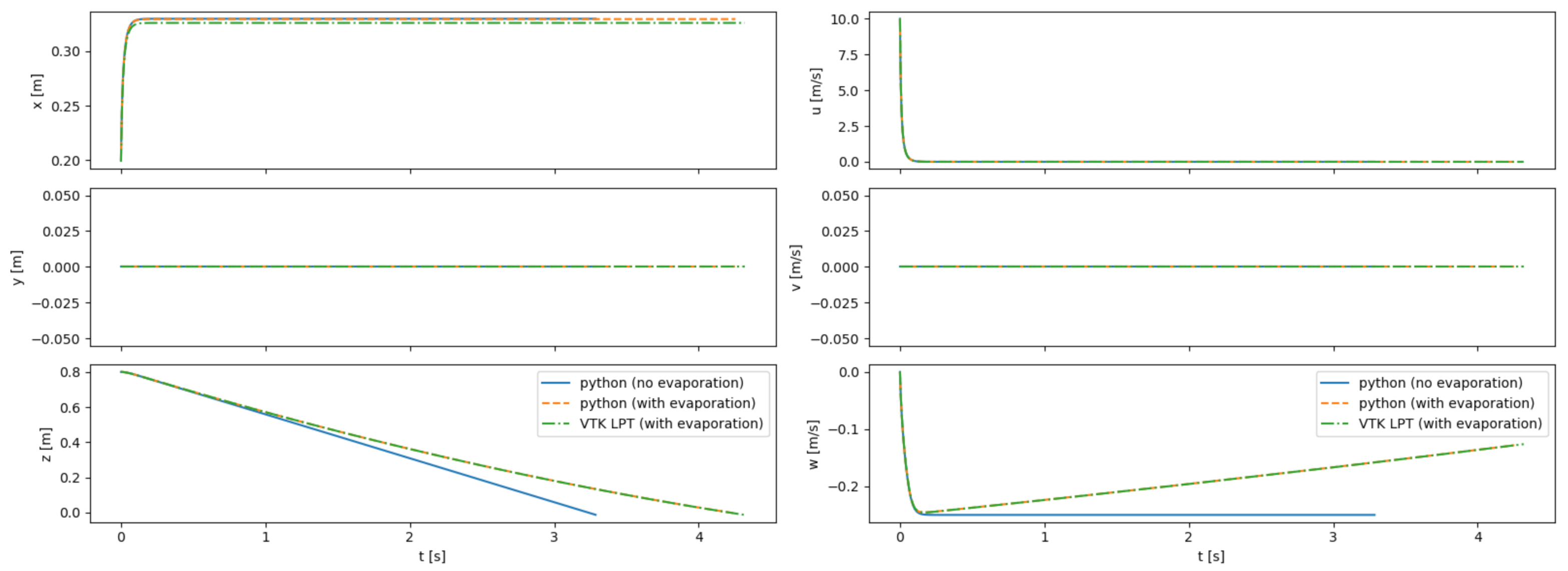
This paper is structured as following: A description of the problem setup and methods, including the bus model, Navier–Stokes flow solver, LPT algorithm, and viral load, are described in Section 2. Section 3 details the validation studies of the flow solver and the LPT algorithms. Section 4 presents results of the study, which are finally summarized in Section 5.

2. Setup and Methods

2.1. Flow Solver

Simulations are performed using RavenCFD, a proprietary Navier–Stokes solver developed by Corvid Technologies. RavenCFD solves the Reynolds-Averaged Navier–Stokes (RANS) equations on an unstructured, arbitrary polyhedral mesh. Simulations are performed using fully implicit time integration based on the methods of [26,27]. Gradients are computed using a weighted least-squares approach and limited using the minmod algorithm (e.g., [28]). Face values are reconstructed using second-order interpolation from cell centers. Inviscid fluxes are computed using the all-speed ‘Low-Diffusion Flux Splitting Scheme’ (LDFSS formulation) of [29], and viscous fluxes are computed using the approach of [26]. Turbulence is modeled using the Shear Stress Transport (SST) model of [30].

Simulations are evolved to steady-state as determined by a reduction in density and turbulent residuals, as well as the convergence of forces on surfaces in the simulation. The final state is determined from time averaging of the last 10 s of simulation time.

2.1.1. Bus Model

A CAD model of a standard Charlotte Area Transit Systems (CATS) bus, as shown in shown in Figure 1, was generated based on detailed measurements performed by the authors, with the assistance of CATS operators and management. The CAD model was then verified against the Gillig low-floor bus model layout obtained from CATS through an NDA between UNC Charlotte and CATS; bus HVAC operating condition data were also obtained through the same NDA. Note that the Gillig low-bus bus model is the most common variant of CATS buses. This bus is approximately $11.6\times 2.4\times 2.5$ m (L × W × H). There are 25 seats for passengers in the main cabin, and the seating at the rear of the bus is elevated.

2.1.2. Passenger Model

CAD models of both seated and standing passengers were created using Corvid Technologies’ proprietary CAVEMAN model, which has previously been used for combat damage mitigation simulations. The passenger models were integrated with the bus model for the various seating and occupancy scenarios described in Section 2.2.2. Figure 2 shows an example of an integrated grid at maximum capacity.

2.1.3. Grid Generation

Conformal grids were created for each bus/passenger combination using a commercial software ANSA by Beta CAE (Luzern, Switzerland).All surfaces were meshed with triangular elements, including the passenger models (Figure 3). Prism layers were grown from the surfaces to capture near-wall gradients, and tetrahedral elements were used in the remaining volumes, see Figure 4. Inside the bus, the maximum cell size (surface and volume) was 25 mm, with additional refinement around the curvature and regions of interest. As shown in Figure 4, on passengers, the maximum surface cell size was 15 mm, with cell sizes of 5 mm near noses and mouths. Volume mesh refinement regions limited volume cell sizes within 100 mm of each passenger to 15 mm.

Initial testing showed that aspect ratio-based layer growth with a first layer aspect ratio of 0.05 produced a high quality near-wall mesh with average wall y+ values of approximately 0.7. This first layer specification was used for all surfaces in all meshes. Due to the complex nature of the interior flow field, the actual y+ values vary significantly and typically range, on average, from 0.3–1.0 for all interior surfaces. It should be noted that for some of the higher-speed flow configurations y+ can exceed 1.0 in the vicinity of source boundary conditions (see Section 2.1.5).

2.1.4. Ambient Conditions

The ambient fluid conditions in the bus are treated as air and initialized to a uniform pressure of $P_{f,0}=\mathrm{101,325}\mathrm{Pa}=1\mathrm{atm}$ and $T_{f,0}=288.15\mathrm{K}=59{}^o\mathrm{F}$. We assume the air is a calorically perfect ideal gas with a ratio of specific heats $\gamma =1.4$ and specific gas constant $R=287.1\mathrm{J}/\left(\mathrm{kg}\mathrm{K}\right)$. This yields a uniform density of ${\rho }_{f,0}=1.225\mathrm{kg}/{\mathrm{m}}^3$.

The dynamic viscosity ${\mu }_{f,0}$ is computed using Sutherland’s law [31], defined as:

$${\mu }_f=\frac{C_1{T}^{3/2}}{T+S}$$

(1)

where $C_1$ and S are constants, defined for air as $C_1=1.458\times {10}^{-6}\mathrm{kg}/\left(\mathrm{m}\mathrm{s}\sqrt{\mathrm{K}}\right)$ and $S=110.4\mathrm{K}$. At the initial bus temperature of $T_{f,0}=288.15\mathrm{K}$, this yields ${\mu }_{f,0}=1.79\times {10}^{-5}\mathrm{kg}/\left(\mathrm{m}\mathrm{s}\right)$.

Table 1. Summary of ambient conditions for the flow solver.

Variable	Definition	Value
$\gamma$	Ratio of specific heats	1.4
R	Specific gas constant	287.1 J/(kg K)
$T_{f,0}$	Initial fluid temperature	288.15 K
$P_{f,0}$	Initial fluid pressure	101,325 Pa
${\rho }_{f,0}$	Initial fluid density	1.225 kg/m${}^3$
${\mu }_{f,0}$	Initial fluid dynamic viscosity	$1.79\times {10}^{-5}$ kg/(m s)

summarizes the ambient conditions for the flow solver.

2.1.5. Boundary Conditions

All surfaces, such as the bus walls, seats, closed windows, and passengers, are treated in the flow solver using an adiabatic no-slip boundary condition. The HVAC registers are modeled as mass flow inlets, which enforce a mass flow rate at a given temperature. The static pressure is extrapolated from the interior of the domain and the fluxes through the boundary are specified directly. Similarly, the HVAC returns are modeled as mass flow outlets. The density, pressure, and velocity are all calculated to provide the specified mass flow rate.

2.2. Flow Considerations

The transport of respiratory particles containing SARS-CoV-2 viruses from an infected passenger is governed by the flow field in the bus. The current study examines the effect of both environmental effects, such as HVAC settings and open windows, as well as mandated COVID-19 interventions by CATS management, such as seating and occupancy restrictions.

2.2.1. HVAC System

When the windows and doors are shut, the internal flow dynamics will be largely determined by the HVAC system. The main cabin HVAC system has multiple registers in the cabin ceiling and a single return at the rear of the bus. The main cabin registers blow air downward from the ceiling. The main HVAC system also feeds a driver cabin register, which also blows downward from the ceiling and can be controlled independently from the main cabin. The front of the bus also has defroster HVAC; the intake is in the driver cabin, and the air is exhausted upward on the front window interior. Four settings are considered here: off, low, medium, and high. The locations of the HVAC system components are shown in Figure 5.

Certain components can be adjusted to increase or decrease the airflow rate inside the bus. The main cabin airflow rate is controlled indirectly by specifying a desired temperature. The airflow rate then adjusts automatically. Five flow rates are considered here for the main cabin registers, based on the maximum possible flow rate: off, 1/4 maximum, 1/2 maximum, 3/4 maximum, and maximum. The driver register can be adjusted independently and has three settings: off, low, and high. Finally, the front defroster has four settings: off, low, medium, and high. To characterize the airflow from the HVAC system inside the CATS bus, air speed measurements were taken by the authors using an anemometer. Up to 14 measurements were performed and averaged for each component. The volume of air contained on the bus is roughly 55 m${}^3$. The HVAC system is capable of up to 140 air changes per hour; i.e., the average parcel of air on the bus will be replaced every 26 s. Results of our measurements are summarized in

Table 2. Summary of HVAC measurements on a CATS bus. Reported values are averages of up to 14 measurements.

HVAC Component	Area (m${}^2$)	Setting	Airspeed (m/s)
Main cabin register	0.08495	Max	4.125
Main cabin return	0.37016	N/A	3.0
Driver area register	0.02065	Low	10.0
		High	20.0
Defroster (blower)	0.03871	Low	5.0
		Med	6.66
		High	8.0
Defroster (return)	0.04935	Low	4.0
		Med	5.3
		High	6.4

.

2.2.2. Seating and Occupancy

In response to the COVID-19 pandemic, CATS has mandated limited seating on buses. To examine the efficacy of these restrictions, we examine multiple seating and occupancy scenarios. We consider passenger arrangements both without and with the current COVID-19 restrictions, as indicated in Figure 6. CATS currently allows passengers to stand, even when all available seats are in use. We therefore consider three occupancy configurations: maximum seated and standing occupancy, maximum seated occupancy (no passengers standing), and half-seated occupancy (no passengers standing). These configurations are also indicated in Figure 6.

2.2.3. Ventilation

Depending on the weather conditions, CATS can open some or all of the windows on the bus. We consider several scenarios: All windows fully shut, all windows fully open, half of the windows fully open, and two mixed configurations labeled as “alternate open A” and “alternate open B”. The first two configurations are obvious, however, the latter three configurations are shown in Figure 7.

When the windows are open, the speed of the bus will alter the flow dynamics. We consider two typical speeds of 25 MPH and 35 MPH. The CATS bus considered for this study also has two doors, a forward and an aft door, that open at the same time. We consider a scenario in which the doors are open, however the bus is not moving. In this case, the wind in the environment around the bus can also affect the internal flow dynamics. We consider two wind speeds of 6 MPH and 12 MPH, based on the average annual wind speed of roughly 8 MPH in Charlotte, NC [32].

2.2.4. Run Groups

Due to the large number of variables considered, the flow simulations are divided into three run groups, labeled A, B, and C, based on the window and door configurations. Run groups A, B, and C are summarized in

Table 3. Summary of run group A, which is performed with all windows and the door closed. A total of 144 flow simulations are performed for group A.

Variable	Values
Windows	all closed
Doors	closed
Bus speed	N/A
Wind speed	N/A
Main cabin HVAC setting	1/4 max, 1/2 max, 3/4 max, max
Driver area HVAC setting	low, high
Defroster setting	low, med, high
Seating restrictions	none, current
Passenger count	max (standing), max (sitting), half

,

Table 4. Summary of run group B, which is performed with some or all windows open and the door closed. A total of 48 flow simulations are performed for group B.

Variable	Values
Windows	all open, half open, config A, config B
Doors	closed
Bus speed	25 MPH, 35 MPH
Wind speed	0 MPH
Main cabin HVAC setting	off
Driver area HVAC setting	off
Defroster setting	off
Seating restrictions	none, current
Passenger count	max (standing), max (sitting), half

, and

Table 5. Summary of run group C, which is performed with all windows closed and the door open. A total of 96 flow simulations are performed for group C.

Variable	Values
Windows	all closed
Doors	open
Bus speed	0 MPH
Wind speed	6 MPH, 12 MPH
Main cabin HVAC setting	1/4 max, 1/2 max, 3/4 max, max
Driver area HVAC setting	low, high
Defroster setting	low, med
Seating restrictions	none, current
Passenger count	max (standing), half

, respectively.

2.3. Lagrangian Particle Tracking

A Lagrangian Particle Tracking (LPT) approach is used to model the transport of SARS-CoV-2 viruses in respiratory droplets. Three injection scenarios are examined for each potential infected bus occupant: speaking, coughing, and sneezing. The injection of particles is modeled as an instantaneous event. The flow conditions are derived from the final time-averaged output of the flow solver.

2.3.1. Particle Dynamics

The trajectories of the particles are evolved using the LPT algorithms in VTK [33], an open-source post-processing and visualization tool. The VTK LPT algorithm uses the formulation of [34]:

$$\begin{array}{cc}\hfill \frac{d{\overrightarrow{x}}_p}{dt}& ={\overrightarrow{u}}_p\hfill \end{array}$$

(2)

$$\begin{array}{cc}\hfill \frac{d{\overrightarrow{u}}_p}{dt}& =\frac{\alpha ({\overrightarrow{u}}_f-{\overrightarrow{u}}_p)}{{\tau }_p}-\overrightarrow{g}(1.0-\frac{{\rho }_f}{{\rho }_p})\hfill \end{array}$$

(3)

where ${\overrightarrow{x}}_p$ is the particle location vector, ${\overrightarrow{u}}_p$ is the particle velocity vector, $\alpha$ is a drag coefficient, ${\tau }_p$ is the particle stopping time, ${\overrightarrow{u}}_f$ is the fluid velocity vector, ${\rho }_f$ is the fluid density, ${\rho }_p$ is the density of the particle, which we assume is constant at roughly the density of water such that ${\rho }_p=1000\mathrm{kg}/{\mathrm{m}}^3$, and $\overrightarrow{g}=[0,0,9.8]\mathrm{m}/{\mathrm{s}}^2$ is the gravitational acceleration vector.

The drag coefficient $\alpha$ is defined as:

$$\alpha =1.0+0.15{\mathrm{Re}}_p^{0.687}$$

(4)

with ${\mathrm{Re}}_p$ the Reynolds number of the particle defined as:

$${\mathrm{Re}}_p=\frac{{\rho }_f|{\overrightarrow{u}}_f-{\overrightarrow{u}}_p|d_p}{{\mu }_f}$$

(5)

where $d_p$ is the particle diameter and ${\mu }_f$ is the dynamic viscosity of the fluid, computed using Sutherland’s Law (Equation (1)).

The particle stopping time ${\tau }_p$ is defined as:

$${\tau }_p=\frac{{\rho }_p{d}_p^2}{18{\mu }_f}.$$

(6)

The trajectories are integrated forward in time using an adaptive fourth order Runge–Kutta algorithm with fifth order correction (RK45). The necessary fluid quantities (density ${\rho }_f$, velocity vector ${\overrightarrow{u}}_f$, and dynamic viscosity ${\mu }_f$) are interpolated from the flow solver output to the particle location at each particle time step.

The stopping time ${\tau }_p$ is a characteristic time over which the relative velocity between the particles and the fluid is brought to zero. In other words, after one or more stopping times, the particle can be assumed to move with the fluid. Figure 8 shows the stopping time as a function of the initial particle diameter at the initial bus flow conditions.

The stopping time is directly proportional to the square of the particle diameter; therefore the smallest particles more rapidly become entrained in the fluid flow. Due to the computational cost associated with modeling the smallest particles using the LPT dynamics, which would limit the timestep to approximately the stopping time, we instead model the smallest particles using the VTK “Streamline” integrator. The streamline integration is similar to the LPT algorithm; however, it is much simpler, as the particle velocity is assumed to be the local fluid velocity, and no drag equation need be solved. Note that this approach neglects gravity, which is a reasonable assumption for the small particles where the gravitational settling time is on the order of minutes or hours, which is much longer than the HVAC air change time (roughly 30 s).

We have verified the accuracy of the use of streamlines by comparing results to LPT trajectories of particles. For particles with initial diameter $d_{p,0}\le 25\mathsf{\mu }\mathrm{m}$, the results obtained with the LPT algorithm and the streamline algorithm are indistinguishable; however, the streamline method required several orders of magnitude fewer iterations, greatly reducing the computational expense. However, for particles with an initial diameter greater than 25 $\mathsf{\mu }\mathrm{m}$, the deviations between the LPT and the streamline integration are apparent. We therefore use the streamline integration for particles $d_{p,0}\le 25$$\mathsf{\mu }\mathrm{m}$, and the LPT algorithm for all larger particles in the size distribution.

The LPT formulation does not include the Brownian motion. In a similar study of SARS-CoV-2 particle transport, [35] estimated that the typical deviation of a respiratory particle due to Brownian motion is approximately 0.03 m in 5000 s, which is negligible compared to the total distance traveled.

2.3.2. Cunningham Slip Correction Factor

Very small particles ($d<1\mu$) require a correction to the drag force known as the Cunningham Slip Correction Factor.

$$C_C=1.0+\mathrm{Kn}(2.514+0.80exp\frac{-0.55}{\mathrm{Kn}})$$

(7)

where $\mathrm{Kn}=\frac{\lambda }{d_p}$ is the Knudsen number, $d_p$ is the particle diameter, and $\lambda$ is the mean free path of the gas (air in our simulation). We neglected small deviations in temperature and pressure in the domain and set the mean free path to be a constant value based on the initial pressure $P_0=\mathrm{101,325}\mathrm{Pa}$ and temperature $T_0=288.15\mathrm{K}$:

$${\lambda }_0=\frac{k_B{T}_0}{\sqrt{2}\pi d_m^2{P}_0}\approx 68\mathrm{\mu }\mathrm{m}$$

(8)

with the average diameter of an air molecule $d_m\approx 0.36\mathrm{nm}$. We have modified the LPT algorithms in VTK to include this factor in the drag law. Note that for large particles, the correction factor is still included but is essentially unity.

2.3.3. Particle Evaporation

The respiratory droplets contain a large amount of volatiles that will evaporate in the air. Evaporation will reduce the effective diameter of the particle and alter the particle dynamics. We have therefore modified the LPT algorithms in VTK to include particle evaporation.

A time-dependent equation for the diameter of respiratory particles is given by [36],

$$d_p\left(t\right)={\left[d_{p,0}^2-8v_m{D}_{{\mathrm{H}}_2\mathrm{O}}\frac{(P_{\mathrm{sat}}-P_{{\mathrm{H}}_2\mathrm{O}})}{k_{B}T}\right]}^{1/2}$$

(9)

where $d_{p,0}$ is the initial diameter of the particle, $v_m=3\times {10}^{-29}{\mathrm{m}}^3$ is the condensed-phase volume occupied by a single water molecule, $D_{{\mathrm{H}}_2\mathrm{O}}=1.8\times {10}^{-5}{\mathrm{m}}^2/\mathrm{s}$ is the molecular diffusivity of water vapor in air, $P_{\mathrm{sat}}$ is the partial pressure of water vapor in equilibrium with the particle surface, $P_{{\mathrm{H}}_2\mathrm{O}}$ is the partial pressure of water vapor in ambient air, T is the temperature, and $k_b=1.38\times {10}^{-23}\mathrm{J}/\mathrm{K}$ is Boltzmann’s constant. $P_{{\mathrm{H}}_2\mathrm{O}}$ is equivalent to $P_{\mathrm{sat}}$ multiplied by the Relative Humidity (RH), $P_{{\mathrm{H}}_2\mathrm{O}}=\left(\mathrm{RH}\right)P_{\mathrm{sat}}$. We treat both the relative humidity and the saturation pressure as constant at $\mathrm{RH}=0.50$ and $P_{\mathrm{sat}}=2320\mathrm{Pa}$.

Following Nicas et al. [36], we approximate the equilibrium diameter of a particle $d_{p,eq}$ to be roughly half of its initial diameter:

$$d_{p,\mathrm{eq}}\approx 0.5d_{p,0}.$$

(10)

Figure 9 shows the time required to reach the equilibrium diameter, $t_{p,eq}$, as a function of the initial diameter. The smallest particles rapidly evaporate to their equilibrium diameter, while the largest particles require substantially more time.

2.3.4. Particle Distributions

Biological particles of saliva and mucus are introduced into the air by means of typical respiratory functions: speaking, coughing, and sneezing. A wide and varying distribution of respiratory particle sizes are generated in each of these events. Although there is substantial variation in the literature on the exact size distribution of the particles, likely due to differences in sample collection, most particles are typically within the range of 1–1000 $\mathsf{\mu }\mathrm{m}$ [35,37,38].

Contraction of viruses can occur through breathing in small particles (≲10 $\mathsf{\mu }\mathrm{m}$) as well as touching contaminated surfaces [36]. This provides motivation to understand the paths of particles with a wide range of diameters to determine ways to reduce the chance of virus contraction.

We independently model three possible injection events: speaking, a cough, and a sneeze. Each event is treated as an instantaneous injection of a given particle size distribution. For speaking and a cough, we use the distributions reported by [39] sampled at a distance of 10 mm. For a sneeze, we use the distribution reported by [40]. For consistency, we resample these distributions to a single distribution given in

Table 6. Particle initial diameter sampling distribution. The average number of particles injected $N_p$ and the average number of copies of the SARS-CoV-2 virus injected $N_v$ are also shown.

Diameter Range $\left[\mathsf{\mu }\mathbf{m}\right]$	LPT Sample Diameter $\left[\mathsf{\mu }\mathbf{m}\right]$	Average ${\mathit{N}}_{\mathit{p}}$ (Speaking)	Average ${\mathit{N}}_{\mathit{v}}$ (Speaking)	Average ${\mathit{N}}_{\mathit{p}}$ (Cough)	Average ${\mathit{N}}_{\mathit{v}}$ (Cough)	Average ${\mathit{N}}_{\mathit{p}}$ (Sneeze)	Average ${\mathit{N}}_{\mathit{v}}$ (Sneeze)
0.0–25.0	streamlines	44.50	2.55	87.66	5.02	936,247.16	53,617.58
25.0–42.5	40	3.56	0.83	4.23	0.99	34,879.55	8181.77
42.5–47.5	45	0.94	0.32	1.11	0.37	5000.65	1670.17
47.5–52.5	50	0.51	0.24	0.57	0.26	2857.52	1309.17
52.5–57.5	55	0.51	0.31	0.57	0.35	2857.52	1742.50
57.5–62.5	60	0.51	0.41	0.57	0.45	2857.52	2262.24
62.5–67.5	65	0.39	0.39	0.43	0.43	1878.82	1891.13
67.5–72.5	70	0.26	0.33	0.28	0.35	900.12	1131.59
72.5–77.5	75	0.26	0.40	0.28	0.43	900.12	1391.81
77.5–82.5	80	0.26	0.49	0.28	0.53	900.12	1689.14
82.5–87.5	85	0.26	0.59	0.28	0.63	900.12	2026.06
87.5–92.5	90	0.30	0.80	0.31	0.83	700.09	1870.59
92.5–97.5	95	0.34	1.07	0.34	1.07	500.07	1571.43
97.5–105.0	100	0.34	1.25	0.34	1.25	500.07	1832.83
105.0–115.0	110	0.68	3.32	0.68	3.32	1000.13	4879.01
115.0–125.0	120	0.65	4.12	0.65	4.12	790.10	5004.08
125.0–135.0	130	0.64	5.15	0.64	5.15	720.09	5798.50
135.0–150.0	140	0.59	5.97	0.77	7.78	673.42	6772.79
150.0–170.0	160	0.91	13.61	2.35	35.23	1066.81	16,015.56
170.0–190.0	180	0.83	17.74	2.01	42.96	940.12	20,095.49
190.0–212.5	200	0.60	17.59	1.00	29.32	560.07	16,422.20
212.5–237.5	225	0.75	31.31	1.25	52.19	700.09	29,227.99
237.5–262.5	250	0.23	13.36	0.35	20.04	350.05	20,046.63
262.5–287.5	275	0.23	17.79	0.35	26.68	350.05	26,682.07
287.5–325.0	300	0.23	23.09	0.35	34.64	350.05	34,640.58
325.0–375.0	350	0.47	73.33	0.70	110.00	700.09	110,015.91
375.0–450.0	400	0.27	62.55	0.44	103.99	416.72	97,751.19
450.0–550.0	500	0.13	61.09	0.37	171.04	266.70	122,188.99
550.0–650.0	600	0.13	105.56	0.37	295.56	266.70	211,142.58
650.0–750.0	700	0.13	167.62	0.37	469.34	266.70	335,286.59
750.0–1000.0	800	0.07	125.11	0.19	350.29	142.69	267,760.07
Total		60.50	758.27	110.10	1774.62	1,001,440.00	1,411,918.24

. Figure 10 compares the cumulative distributions of the references with the resampled distributions used in this study. Figure 11 compares the number of particles in each diameter sampling interval between the references and this study.

Table 7. Summary of particle injection event parameters. For the distributions from [39], we use the samples collated at a distance of 10 mm.

Event	Distribution Reference	Injection Speed [38]
Speaking	[39]	1 m/s
Cough	[39]	10 m/s
Sneeze	[40]	35 m/s

summarizes the particle injection speeds and diameter distributions.

2.3.5. Viral Mean Exposure Time

To enable comparison of the numerous runs and infection mitigation strategies, the relative amount of exposure to viruses is quantified using a volumetric Mean Exposure Time (MET) [41,42,43]. This quantity is similar to a Particle Residence Time (PRT) and is defined over a discrete element.

We define the Viral MET (VMET) at a discrete volume element e as:

$$\mathrm{VMET}\left(\mathrm{e}\right)=\frac{1}{{\left(V_e\right)}^{(1/3)}}\sum _{p=1}^{N_p}{N}_v\left(p\right){\int }_{t=0}^{\infty }{\chi }_e(p,t)dt$$

(11)

where $V_e$ is the volume of element e, $N_p$ is the total number of particles injected, ${\chi }_e(p,t)$ is a sharp Heaviside function defined as unity if particle p resides in the volume $V_e$ at time t and zero otherwise, and $N_v\left(p\right)$ is the estimated number of SARS-CoV-2 viruses in particle p.

We assume that SARS-CoV-2 viruses are initially uniformly distributed in a given volume of respiratory fluid, at a constant number density of $n_v=7\times {10}^{12}\mathrm{copies}/{\mathrm{m}}^3$ [44]. Note that this is an average viral load; the maximum number of copies can be orders of magnitude greater [44]. Furthermore, we assume that the viruses are not evaporated but remain in the particle; therefore the number of viruses in a given particle is purely a function of its initial diameter:

$$N_v\left(p\right)=\frac{4}{3}\pi n_v{\left(\frac{d_{p,0}}{2}\right)}^3.$$

(12)

Figure 12 shows the number of viruses released in each injection event in each diameter range sampled.

We note that our definition of VMET (Viral Mean Exposure Time) differs from the MET of [41] in two ways. First, we include the viral load in the definition because we are focused on the risk of transmission of COVID-19. This weighs the exposure to a larger particle more heavily than a smaller particle, as the larger particle contains a greater number of copies of the SARS-CoV-2 virus. Second, Duvernois et al. [41] included a normalizing factor based on the number of unique ‘encounters’ of a particle with a volume element. The authors noted that this resulted in recirculating particles, contributing less to the MET than a stagnant particle. While this may be true in some circumstances, we do not see a need to include this factor, as our volume elements are quite small and recirculation can still result in exposure.

To compute the VMET, we first resample the particle trajectories to a uniform time step of $\Delta t=0.001\mathrm{s}$. To obtain consistent volume elements, we compute the VMET on a uniform Cartesian grid of cell length $\Delta x=0.01\mathrm{m}$. These two steps ensure that no particle will move more than one cell length in a given timestep based on the maximum particle injection speed is 35 m/s. The volumetric VMET computed on the structured grid can then be resampled back to the unstructured grid used in the flow solver for visualization and analysis. The VMET is a cell-centered quantity with units of viral copies multiplied by time per length (e.g., copies-s/m). Intuitively, the VMET represents the average amount of viruses present in a given volume element when sampled over a finite amount of time. The greater the VMET, the higher the risk of exposure to SARS-CoV-2.

We also note that the VMET is not normalized by the total amount of viruses in the injection event. A sneeze produces roughly 10,000 times more respiratory particles than speaking or coughing (and correspondingly 1000 times more viruses) and is therefore potentially much more dangerous. Our definition of VMET captures this when comparing injection events.

2.4. A Note on Post-Processing

ParaView [45] is a powerful open-source tool for flow visualization. The latest version of ParaView can be found on the website (http://www.paraview.org/download, accessed on 5 January 2021). The majority of processing was completed using version ParaView v5.7.0; however, general post processing of solutions may be accomplished with any version that has the eXtensible Data Model and Format (XDMF) reader (for CFD solutions) or Visual Took Markup Language (VTML) reader (for viral load solutions). The authors intend to make the simulation data sets available to researchers interested to investigate viral-particle flows for scenarios other than those presented in this paper. For that matter, a brief description of a general flow, or pipeline, for visualizing and post-processing CFD solutions is outlined below:

• Step 1: Load XDMF data file;
• Step 2: Pick appropriate variables and mesh components (volume/surface) to load and apply;
• Step 3: Extract surfaces;
• Step 4: Extract volume.

From this point, the surface and volume elements are available to interrogate however the user wishes, e.g., coloring surfaces by pressure or seeding streamlines in the volumes. A similar approach is taken for the viral load data, which is stored in a VTML format file. However, there are no surface data elements in the VTML files; only volumetric field data. Any surface visualization that is desired must be completed using the XMDF files; note that these can be included in the same pipeline and overlaid. The Viral Mean Exposure Time (VMET) (Equation (11)) is stored as field data in the VTML files, labeled as the person number followed by the type of injection event (speaking, cough, or sneeze). The viral load data can be sliced, as in Figure 13, thresholded, or rendered volumetrically.

3. Validation and Grid Convergence

3.1. Flow Solver Validation

To validate the ability of RavenCFD to simulate low-speed flows, we compared with the results of Hooff et al. [46]. The authors presented both experimental and simulation results of cross-ventilation flow through an isolated building. Similar results are reported in Ramponi & Blocken [47] and Karava et al. [48].

A building of dimensions $0.2\times 0.2\times 0.16{\mathrm{m}}^3$ is placed in a computational domain of extent $2.16\times 1.8\times 0.96{\mathrm{m}}^3$. The building has an open window of area $3.3\times {10}^{-3}{\mathrm{m}}^2$ on both the windward and leeward walls.

The flow is injected into the domain with a vertical power-law profile designed to match the experimental wind tunnel; see Equation 1 of Hooff et al. [46]. The velocity is normalized using a reference velocity of $U_{H}H=4.3\mathrm{m}/\mathrm{s}$ which is computed at the building height $H=0.16\mathrm{m}$.

RANS simulations are performed in RavenCFD using the SST model of Menter [30]. The turbulent kinetic energy k and specific dissipation rate $\omega$ are also initialized with a vertical profile; see Equations 2–5 of Hooff et al. [46].

Simulations are evolved to steady-state, as determined by a reduction of density residuals and by convergence of the forces and moments on the building. The results are time-averaged over 7 s.

Qualitatively, the authors identify several flowfield features in the RANS simulations of Hooff et al. [46]. First, the flow entering the building through the windward window creates a jet that points downward and spreads with a characteristic width. Second, the flow leaving building creates a jet the points upward and also spreads with a characteristic width. Finally, the impinging flow on the top of the building creates a stagnation region. It is worth noting that none of the RANS methods considered in Hooff et al. [46] captured the vertical jet flapping observed in the experiments and LES simulations. Despite this, the authors find that the RANS models do sufficiently capture the volume flow rates and general flow dynamics.

For comparison to experimental results, the horizontal velocity profile is extracted at various locations inside the building. Figure 14 shows the experimental and SST simulation results of Hooff et al. [46], as well as the RavenCFD SST results. Overall, the RavenCFD results show good agreement with both the experimental measurements and the SST results of Hooff et al. [46], providing high confidence in the ability of RavenCFD to model subsonic cross-flow scenarios similar to those on the CATS bus.

3.2. Lagrangian Particle Tracking Validation

The Lagrangian particle tracking (LPT) algorithm in VTK, including the modifications described above to include the Cunningham slip correction factor and the evaporation model, are validated by comparing to results obtained with an external ODE solver implemented in Python. The external solver uses the “ivp_solve” routine from the “scipy” package.

Particle trajectories are simulated in an empty room with either static or uniform flow. Particles are injected from a known position and with constant velocity. Figure 15 shows a comparison between the results obtained with the Python code with the VTK LPT results for a single particle injected into static flow. The LPT results from VTK are nearly identical to the results obtained with the external tool, providing high confidence in the ability of VTK to model the particles as well as validating our modifications to the VTK code to include evaporative effects and the Cunningham correction factor.

3.3. Grid Convergence Test

A grid resolution study was performed on a filled bus model, with velocity profiles extracted and compared along each of the green columns visualized in Figure 16. For ease of mesh generation, all meshes were unstructured. Each of the grids included near-wall prism layers to ensure proper resolution of the low-Re boundary layers that manifests in regions of higher velocities. All surface generated grids leverage a minimum internal angle of 18${}^{\circ }$ and an Equiarea skewness (see Ansys User Guide [49]) of 0.5. All volume grids have target quality metrics of a 0.4 solid Jacobian, a cell skewness (see OpenFOAM User Guide [50]) of 4, and a maximum volume ratio of 105. The grid was progressively refined starting at a 39 million element grid for the coarse mesh, a 54 million element grid for the medium, and a 106 million element grid as the fine. A subset of the results extracted from the columns shown in Figure 16 is shown in Figure 17 and includes results of flow variation in the $X-$, $Y-$, and Z-Velocity. Based on the results shown, the meshes in the present study leverage the fine grid level of refinement. While cell counts varied depending on occupancy, each grid used contained roughly 100 million elements, including the additional refinements in the near proximity of each occupant.

4. Results

Due to the number of cases considered as a part of the current study, all cases have not yet been thoroughly interrogated. In order to provide some perspective on the solution contents, we share preliminary observations by comparing a windows closed case with arbitrarily selected HVAC settings to the windows fully open and half open cases at 35 MPH.

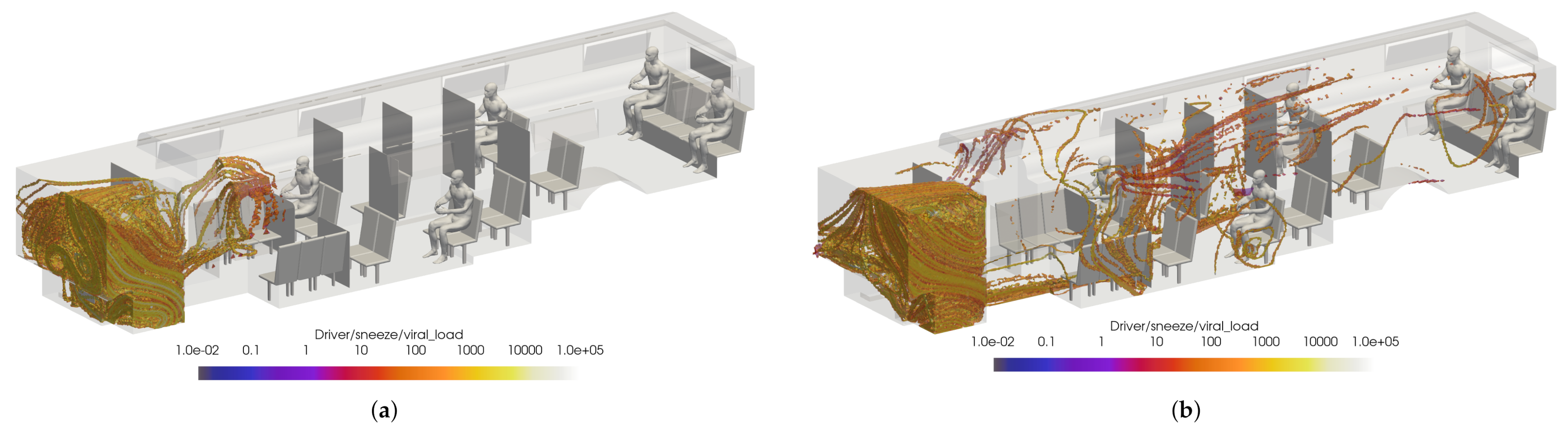
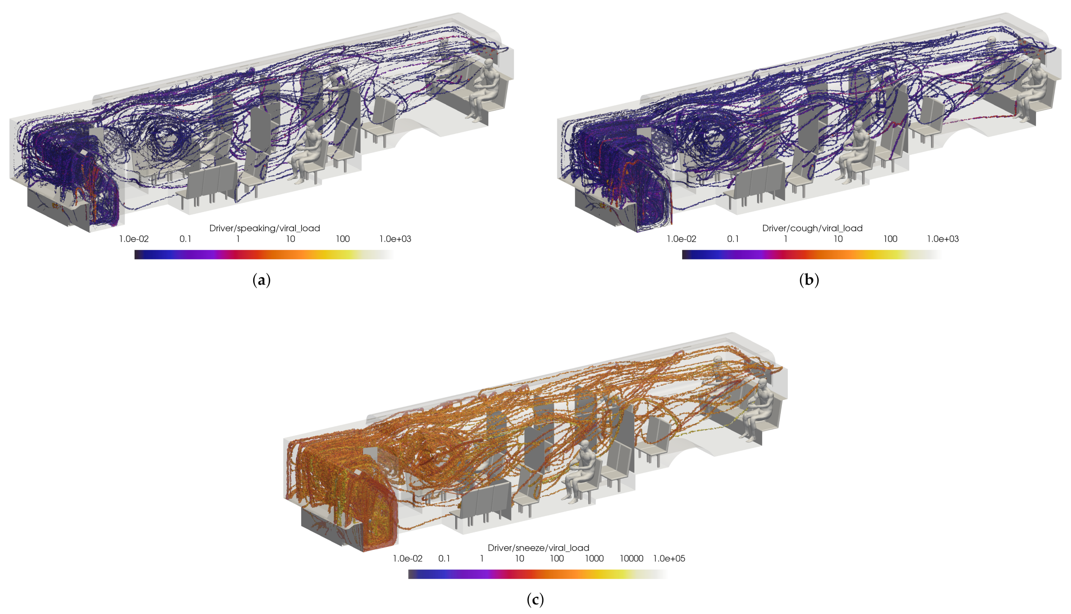
Preliminary results are shown for a case with windows and doors closed, at half-seated occupancy under COVID-19 restrictions, with the main HVAC at a maximum flow rate, the driver HVAC on low, and the defroster on medium. The VMET is presented for injection events from the bus driver to show a comparison of the three types of events: speaking, coughing, and sneezing.

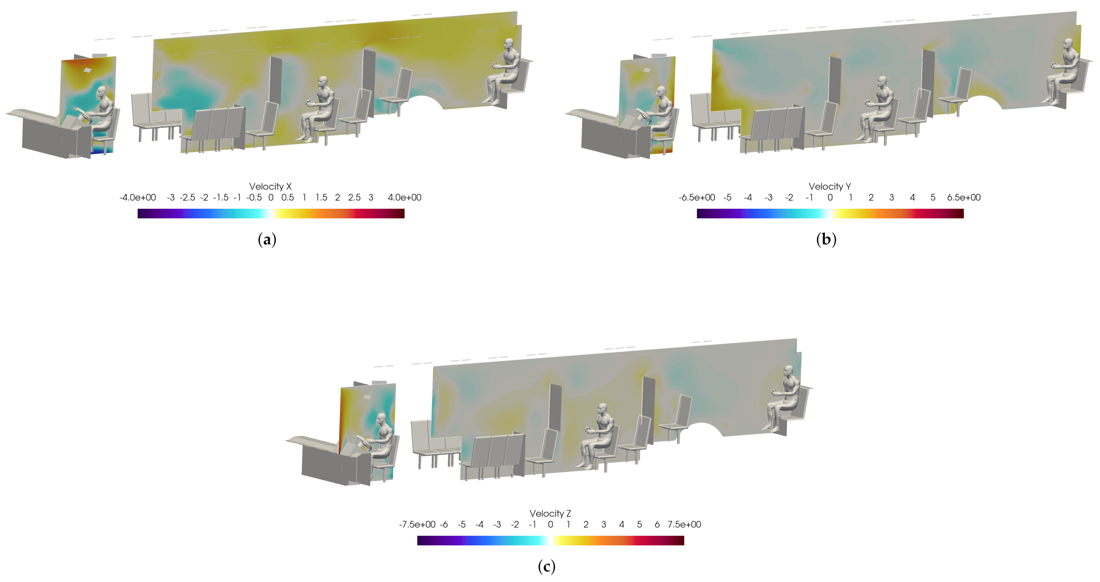
Figure 18 shows slices taken through the domain and centered on the driver. It can be seen in Figure 18a that the overall flow is toward the rear of the bus, as indicated by the positive x-direction velocity. Also, Figure 18c shows that the injection of air from the defroster is also clearly visible in the z-direction velocity. For all injection events, the viral load is most concentrated in the area immediately in front of the driver. This is because most of the viral load is contained in the largest particles which have the most inertia and are therefore least affected by the flow dynamics; they are also the largest and therefore drop rapidly due to gravity.

Figure 19 shows a volumetric threshold in the domain, which identifies any cells with a non-zero VMET. Although the viral load is concentrated in the area surrounding the driver, there is still an exposure risk from the smaller particles (i.e., aerosols) that are entrained in the flow and can spread throughout the bus. The smallest particles are correspondingly light and do not rapidly drop to the ground. The overall flow dynamics in the bus with the windows and doors closed is directed toward the rear of the bus, which is where the main HVAC return is located. This can be seen in Figure 20, where the positive velocity in the x-direction indicates flow toward the rear of the bus. Therefore the aerosolized particles will migrate backwards from the driver.

To help determine the best HVAC/window configuration for CATS, the previous case was compared to cases with the windows fully open and half open with the HVAC off. The VMET was presented for a sneeze injection event for the driver. Figure 21 shows the comparison of the volumetric threshold for the driver’s sneeze for each case. For both the windows fully open and half open cases, the VMET for the driver remains largely the same. While the viral load is more concentrated in the area surrounding the driver, there is no flow directed toward the rear of the bus as the AC remains off and the particles are instead ejected from the window just rear of the driver.

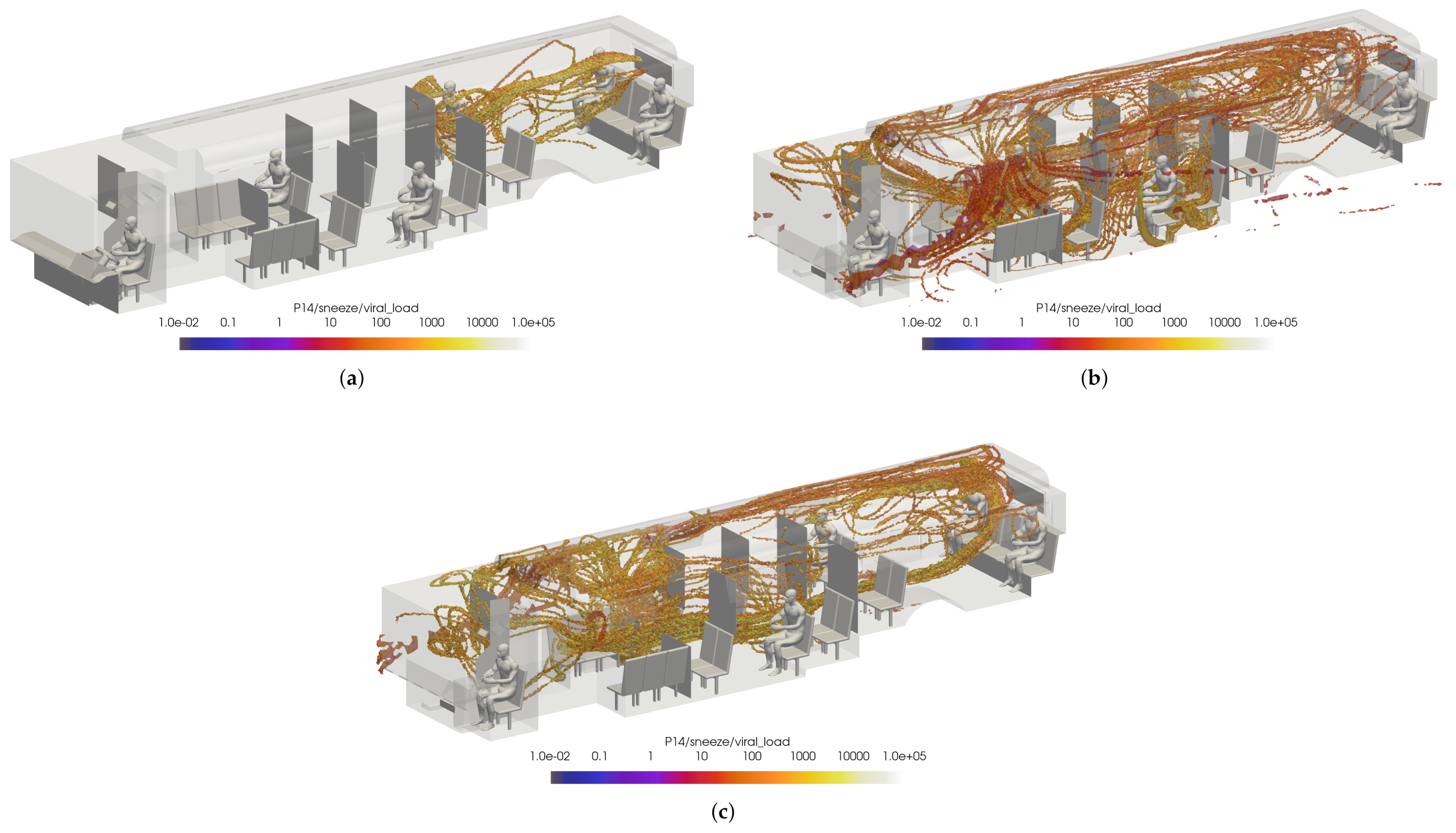
While this initially leads to the conclusion that the windows fully/half open cases are better for the prevention viral transmission, this does not represent the overall flow dynamics in the bus. To ensure incorrect conclusions were not drawn, two passengers were arbitrarily selected for comparison: passenger 14 and passenger 15. Once again, the VMET was presented for a sneeze injection event. Figure 22 shows the comparisons of the volumetric threshold for passenger 14’s sneeze for each case. For the windows closed case, passenger 14’s aerosols largely move towards the rear of the bus where the main HVAC return is located. In contrast, the windows fully open case shows the aerosols circulating throughout the entire bus. This is a result of the increased turbulence within the bus from having multiple competing inlets in the form of open windows. The windows half open case shows a similar result, only to a slightly lesser degree. 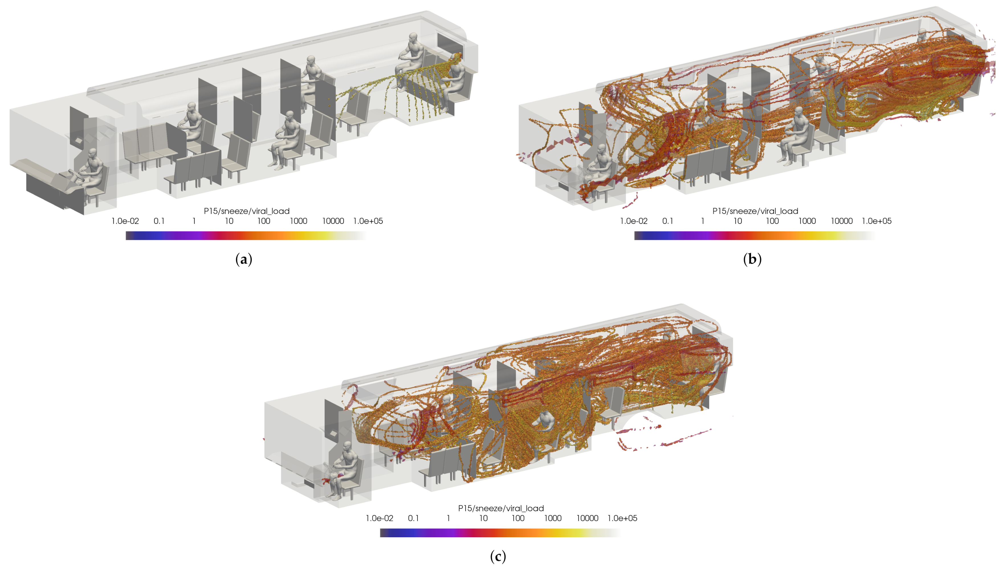Figure 23 shows the comparisons of the volumetric threshold for passenger 15’s sneeze for each case. The results are comparable to those for passenger 14, with the windows closed case directing a majority of the particles aside from the initial injection into the HVAC return. Both cases with windows open similarly show an increase in circulation of aerosols, with the windows fully open case again circulating more of the particles with a higher VMET.

With a significant number of cases yet to be investigated, it is difficult at this time to recommend a complete configuration of HVAC and windows open/closed for the best prevention of viral transmission. However, from these initial cases it seems that the spread of viral particles from infected passengers is reduced with the windows closed and the cabin HVAC set to high. This is a result of the positive velocity in the x-direction directing the particles toward the main HVAC return rather than circulating the particles throughout the bus due to the increased turbulence in the flow field from open windows. In contrast, it seems that both windows open cases reduce the spread of viral particles from the driver. It is possible that keeping the majority of the windows closed, however leaving the window just rear of the driver open could lead to a best case scenario. However, it is also possible that having the driver HVAC off is contributing to the lack of circulation. To isolate this phenomena, one more case was observed. The alternate configuration B for the windows half open case has the same HVAC settings as both previous windows open cases, but has the window behind the driver closed. Figure 24 shows the comparison of the volumetric threshold for the driver’s sneeze for the windows half open and alternate open B cases. This clearly demonstrates that having the window just rear of the driver open can significantly limit the spread of the driver’s aerosols in most cases. While these preliminary results show a general trend of best practices, there are still many other cases to compare.

5. Conclusions

In this research effort, our team developed a high-fidelity database of scenarios that relate to operation in a Charlotte Area Transit System Bus. High-fidelity Navier–Stokes solutions were developed for a range of configurations, HVAC settings, and operational settings. An open-source Lagrangian particle tracking method was modified to include evaporative effects and used to simulate the trajectories of respiratory particles injected into the flow via speaking, coughing, and sneezing. The trajectories were then mapped to quantify the average risk of exposure to the SARS-CoV-2 virus across all considered flow scenarios. This viral exposure map provides insight into the common areas of virus collection across all configurations and settings which may be leveraged to better understand viral transmission and thus establish procedural changes that can mitigate the spread of COVID-19, and other aerosolized virus particles.

References

1. Shen, Y.; Li, C.; Dong, H.; Wang, Z.; Martinez, L.; Sun, Z.; Handel, A.; Chen, Z.; Chen, E.; Ebell, M.H.; et al. Community outbreak investigation of SARS-CoV-2 transmission among bus riders in eastern China. JAMA Intern. Med. 2020, 180, 1665–1671. [Google Scholar] [CrossRef] [PubMed]
2. Shen, Y.; Li, C.; Dong, H.; Wang, Z.; Martinez, L.; Sun, Z.; Handel, A.; Chen, Z.; Chen, E.; Ebell, M.; et al. Airborne Transmission of COVID-19: Epidemiologic Evidence from Two Outbreak Investigations. 2020. preprint. Available online: https://www.researchgate.net/publication/340418430_Airborne_transmission_of_COVID-19_epidemiologic_evidence_from_two_outbreak_investigations (accessed on 29 April 2021).
3. Shen, Y.; Li, C.; Ling, F. Community outbreak investigation of SARS-CoV-2 transmission among bus riders in eastern China—More detailed studies are needed—Reply. JAMA Intern. Med. 2021, 181, 719–720. [Google Scholar] [CrossRef] [PubMed]
4. Mallapaty, S. What the cruise-ship outbreaks reveal about COVID-19. Nature 2020, 580, 18–19. [Google Scholar] [CrossRef] [PubMed] [Green Version]
5. Azimi, P.; Keshavarz, Z.; Laurent, J.G.C.; Stephens, B.; Allen, J.G. Mechanistic transmission modeling of COVID-19 on the Diamond Princess cruise ship demonstrates the importance of aerosol transmission. Proc. Natl. Acad. Sci. USA 2021, 118, e2015482118. [Google Scholar] [CrossRef]
6. McCartney, S. The Key to Safe Airflow for Planes before Takeoff. The Wall Street Journal. 7 April 2021. Available online: https://www.wsj.com/articles/the-key-to-safe-airflow-for-planes-before-takeoff-11617800215?st=j3mzpfpzp2h0uyi&reflink=desktopwebshare (accessed on 29 April 2021).
7. Schwartz, S. Public Transit and COVID-19 Pandemic: Global Research and Best Practices; American Public Transportation Association: Washington, DC, USA, 2020. [Google Scholar]
8. Zhu, S.; Srebric, J.; Spengler, J.D.; Demokritou, P. An advanced numerical model for the assessment of airborne transmission of influenza in bus microenvironments. Build. Environ. 2012, 47, 67–75. [Google Scholar] [CrossRef]
9. Gurley, G. Reducing Risks in the Air on Buses. The American Prospect. 15 July 2020. Available online: https://prospect.org/coronavirus/reducing-risks-in-the-air-on-buses (accessed on 29 April 2021).
10. Yang, X.; Ou, C.; Yang, H.; Liu, L.; Song, T.; Kang, M.; Lin, H.; Hang, J. Transmission of pathogen-laden expiratory droplets in a coach bus. J. Hazard. Mater. 2020, 397, 122609. [Google Scholar] [CrossRef]
11. Kale, S.; Veeravalli, S.; Punekar, H.; Yelmule, M. Air flow through a non-airconditioned bus with open windows. Sadhana 2007, 32, 347–363. [Google Scholar] [CrossRef]
12. Li, F.; Lee, E.S.; Zhou, B.; Liu, J.; Zhu, Y. Effects of the window openings on the micro-environmental condition in a school bus. Atmos. Environ. 2017, 167, 434–443. [Google Scholar] [CrossRef]
13. Chaudhry, S.K.; Elumalai, S.P. The influence of school bus ventilation scenarios over in-cabin PM number concentration and air exchange rates. Atmos. Pollut. Res. 2020, 11, 1396–1407. [Google Scholar] [CrossRef]
14. Zhang, Z.; Han, T.; Yoo, K.H.; Capecelatro, J.; Boehman, A.L.; Maki, K. Disease transmission through expiratory aerosols on an urban bus. Phys. Fluids 2021, 33, 015116. [Google Scholar] [CrossRef]
15. Edwards, N.J.; Widrick, R.; Wilmes, J.; Breisch, B.; Gerschefske, M.; Sullivan, J.; Potember, R.; Espinoza-Calvio, A. Reducing COVID-19 Airborne Transmission Risks on Public Transportation Buses: An Empirical Study on Aerosol Dispersion and Control. Aerosol Sci. Technol. 2021, 55, 1378–1397. [Google Scholar] [CrossRef]
16. Silcott, D.; Kinahan, S.; Santarpia, J.; Silcott, B.; Silcott, P.; Silcott, B.; Distelhorst, S.; Herrera, V.; Rivera, D.; Crown, K.; et al. TRANSCOM/AMC Commercial Aircraft Cabin Aerosol Dispersion Tests; Technical Report; National Strategic Research Institute: Lincoln, NE, USA, 2020. [Google Scholar]
17. Moreno, T.; Pintó, R.M.; Bosch, A.; Moreno, N.; Alastuey, A.; Minguillón, M.C.; Anfruns-Estrada, E.; Guix, S.; Fuentes, C.; Buonanno, G.; et al. Tracing surface and airborne SARS-CoV-2 RNA inside public buses and subway trains. Environ. Int. 2021, 147, 106326. [Google Scholar] [CrossRef]
18. Green, D.; Zhou, J.; Desouza, C. Transport For London SARS-CoV-2 RNA Sampling Study; Environmental Research Group, Imperial College London: London, UK, 2021. Available online: https://content.tfl.gov.uk/covidsampling-paper-phase-1.pdf (accessed on 29 April 2021).
19. Grondahl, M.; Goldbaum, C.; White, J.; Lohner, R. What Happens to Viral Particles on the Subway. The New York Times. 10 August 2020. Available online: https://www.nytimes.com/interactive/2020/08/10/nyregion/nyc-subway-coronavirus.html (accessed on 29 April 2021).
20. Jones, L.D.; Chan, E.R.; Zabarsky, T.F.; Cadnum, J.L.; Navas, M.E.; Redmond, S.N.; Kovach, J.D.; Linger, M.; Rutala, W.A.; Zimmerman, P.A.; et al. Transmission of SARS-CoV-2 on a Patient Transport Van. Clin. Infect. Dis. 2021, 74, 339–342. [Google Scholar] [CrossRef]
21. Mathai, V.; Das, A.; Bailey, J.A.; Breuer, K. Airflows inside passenger cars and implications for airborne disease transmission. Sci. Adv. 2021, 7, eabe0166. [Google Scholar] [CrossRef]
22. Sugiura, N. Study: Opening windows not best defense against droplets in car. The Asian Shimbun. 27 November 2020. Available online: http://www.asahi.com/ajw/articles/13968048 (accessed on 29 April 2021).
23. Feng, Y.; Zhao, J.; Spinolo, M.; Lane, K.; Leung, D.; Marshall, D.; Mlinaric, P. Assessing the filtration effectiveness of a portable ultraviolet air cleaner on airborne SARS-CoV-2 laden droplets in a patient room: A numerical study. Aerosol Air Qual. Res. 2021, 21, 200608. [Google Scholar] [CrossRef]
24. Yao, F.; Liu, X. The effect of opening window position on aerosol transmission in an enclosed bus under windless environment. Phys. Fluids 2021, 33, 123301. [Google Scholar] [CrossRef]
25. Ou, C.; Hu, S.; Luo, K.; Yang, H.; Hang, J.; Cheng, P.; Hai, Z.; Xiao, S.; Qian, H.; Xiao, S.; et al. Insufficient ventilation led to a probable long-range airborne transmission of SARS-CoV-2 on two buses. Build. Environ. 2022, 207, 108414. [Google Scholar] [CrossRef]
26. Grismer, M.J.; Strang, W.Z.; Tomaro, R.F.; Witzeman, F.C. Cobalt: A parallel, implicit, unstructured Euler/Navier–Stokes solver. Adv. Eng. Softw. 1998, 29, 365–373. [Google Scholar] [CrossRef]
27. Strang, W.; Tomaro, R.; Grismer, M. The defining methods of Cobalt-60—A parallel, implicit, unstructured Euler/Navier–Stokes flow solver. In Proceedings of the 37th Aerospace Sciences Meeting and Exhibit, Reno, NV, USA, 11–14 January 1999; American Institute of Aeronautics and Astronautics: Reston, VA, USA, 1999. [Google Scholar] [CrossRef]
28. Roe, P. Characteristic-Based Schemes for the Euler Equations. Annu. Rev. Fluid Mech. 1986, 18, 337–365. [Google Scholar] [CrossRef]
29. Edwards, J.R. Towards unified CFD simulations of real fluid flows. In Proceedings of the 15th AIAA Computational Fluid Dynamics Conference, Anaheim, CA, USA, 11–14 June 2001; American Institute of Aeronautics and Astronautics: Anaheim, CA, USA, 2001. [Google Scholar] [CrossRef]
30. Menter, F.R. Two-equation eddy-viscosity turbulence models for engineering applications. AIAA J. 1994, 32, 1598–1605. [Google Scholar] [CrossRef] [Green Version]
31. Sutherland, W. LII. The viscosity of gases and molecular force. Lond. Edinb. Dublin Philos. Mag. J. Sci. 1893, 36, 507–531. [Google Scholar] [CrossRef] [Green Version]
32. NOAA/NCDC. Climatic Wind Data for the United States; Technical Report; NOAA: Asheville, NC, USA, 1998. [Google Scholar]
33. Schroeder, W.; Martin, K.; Lorensen, B. The Visualization Toolkit; Kitware: Clifton Park, NY, USA, 2006. [Google Scholar]
34. Matida, E.A.; Finlay, W.H.; Lange, C.F.; Grgic, B. Improved numerical simulation of aerosol deposition in an idealized mouth – throat. J. Aerosol Sci. 2004, 35, 1–19. [Google Scholar] [CrossRef]
35. Zhao, L.; Qi, Y.; Luzzatto-fegiz, P.; Cui, Y.; Zhu, Y. COVID-19: Effects of Environmental Conditions on the Propagation of Respiratory Droplets. Nano Lett. 2020, 20, 7744–7750. [Google Scholar] [CrossRef] [PubMed]
36. Nicas, M.; Nazaroff, W.W.; Hubbard, A. Toward Understanding the Risk of Secondary Airborne Infection: Emission of Respirable Pathogens. J. Occup. Environ. Hyg. 2010, 2, 143–154. [Google Scholar] [CrossRef]
37. Gralton, J.; Tovey, E.; McLaws, M.L.; Rawlinson, W.D. The role of particle size in aerosolised pathogen transmission: A review. J. Infect. 2011, 62, 1–13. [Google Scholar] [CrossRef]
38. Chen, C.; Zhao, B. Some questions on dispersion of human exhaled droplets in ventilation room: Answers from numerical investigation. Indoor Air 2010, 20, 95–111. [Google Scholar] [CrossRef]
39. Chao, C.Y.H.; Wan, M.P.; Morawska, L.; Johnson, G.R.; Ristovski, Z.D.; Hargreaves, M.; Mengersen, K.; Corbett, S.; Li, Y.; Xie, X.; et al. Characterization of expiration air jets and droplet size distributions immediately at the mouth opening. J. Aerosol Sci. 2009, 40, 122–133. [Google Scholar] [CrossRef] [Green Version]
40. Duguid, J.P. The size and the duration of air-carriage of respiratory droplets and droplet-nuclei. Epidemiol. Infect. 1946, 44, 471–479. [Google Scholar] [CrossRef] [Green Version]
41. Duvernois, V.; Marsden, A.L.; Shadden, S.C. Lagrangian analysis of hemodynamics data from FSI simulation. Int. J. Numer. Methods Biomed. Eng. 2013, 29, 1–25. [Google Scholar] [CrossRef] [Green Version]
42. Kunov, M.J.; Steinman, D.A.; Ethier, C.R. Particle Volumetric Residence Time Calculations in Arterial Geometries. J. Biomech. Eng. 1996, 118, 158–164. [Google Scholar] [CrossRef]
43. Lonyai, A.; Dubin, A.M.; Feinstein, J.A.; Taylor, C.A.; Shadden, S.C. New Insights into Pacemaker Lead-Induced Venous Occlusion: Simulation-Based Investigation of Alterations in Venous Biomechanics. Cardiovasc. Eng. 2010, 10, 84–90. [Google Scholar] [CrossRef]
44. Wölfel, R.; Corman, V.M.; Guggemos, W.; Seilmaier, M.; Zange, S.; Müller, M.A.; Niemeyer, D.; Jones, T.C.; Vollmar, P.; Rothe, C.; et al. Virological assessment of hospitalized patients with COVID-2019. Nature 2020, 581, 465–469. [Google Scholar] [CrossRef] [Green Version]
45. Ahrens, J.; Geveci, B.; Law, C. ParaView: An End-User Tool for Large Data Visualization. In Visualization Handbook; Elsevier: Amsterdam, The Netherlands, 2005. [Google Scholar]
46. Hooff, T.V.; Blocken, B.; Tominaga, Y. On the accuracy of CFD simulations of cross-ventilation flows for a generic isolated building: Comparison of RANS, LES and experiments. Build. Environ. 2017, 114, 148–165. [Google Scholar] [CrossRef]
47. Ramponi, R.; Blocken, B. CFD simulation of cross-ventilation for a generic isolated building: Impact of computational parameters. Build. Environ. 2012, 53, 34–48. [Google Scholar] [CrossRef]
48. Karava, P.; Stathopoulos, T.; Athienitis, A.K. Airflow assessment in cross-ventilated buildings with operable façade elements. Build. Environ. 2011, 46, 266–279. [Google Scholar] [CrossRef]
49. Fluent, A. Release 14.0, User Guide; ANSYS, Inc.: Lebanon, PA, USA, 2011; pp. 2385–2394. [Google Scholar]
50. Greenshields, C. OpenFOAM User Guide; Version 3; OpenFOAM Foundation Ltd.: London, UK, 2019. [Google Scholar]
Figure 1. CAD model of the Charlotte Area Transit System (CATS) bus generated based on measurements by the authors. (a): Starboard side view; (b) port side view.
Fluids 07 00080 g001aFluids 07 00080 g001b
Figure 2. Integrated bus and passenger models for a bus at maximum occupancy. (a) Front view; (b) side view.
Fluids 07 00080 g002
Figure 3. Example of triangular surface mesh on a bus passenger model generated using ANSA.
Fluids 07 00080 g003
Figure 4. Slice through the volume mesh generated using ANSA. Prism layers are visible, extending from surfaces, including occupants. Additional refinement is also included around occupants.
Fluids 07 00080 g004
Figure 5. Location of modeled HVAC components; registers are colored pink, and returns are colored blue. (a) Main cabin; (b) driver; (c) defroster.
Fluids 07 00080 g005
Figure 6. Map of bus interior showing the location and numbering convention of passengers (a) without and (b) with the current COVID-19 occupancy restrictions. Note that passengers 31 and 32 are only included in simulations in which the doors are open. In the half-seated configuration, only the blue-seated passengers are present.
Fluids 07 00080 g006
Figure 7. Map of bus interior showing the location and configuration of windows.
Fluids 07 00080 g007
Figure 8. The stopping time τ p as a function of initial particle diameter d p , 0 . The particle density is constant at ρ p = 1000 kg / m 3 . The fluid dynamic viscosity μ f is computed using Sutherland’s Law (see Equation (1)) at the initial bus temperature T f , 0 = 288.15 K .
Fluids 07 00080 g008
Figure 9. The time required to reach the equilibrium diameter, d ( t p , e q ) = d p , e q = 0.5 d p , 0 , as a function of initial particle diameter d p , 0 .
Fluids 07 00080 g009
Figure 10. Comparison of cumulative particle number distributions between the source data in Refs. [39,40] and the resampled size distributions for this study.
Fluids 07 00080 g010
Figure 11. Particle number distributions of initial particle diameter d p , 0 . The data from Refs. [39,40] is resampled to a finer particle size distribution for this study. Note that the number of particles reported is a sum over each sampled diameter range.
Fluids 07 00080 g011
Figure 12. Number of copies of SARS-CoV-2 virus injected as a function of initial particle diameter d p , 0 . We assume a viral load of 7 × 10 12 copies / m 3 based on [44]. The number of viruses reported is a sum over each sampled diameter range.
Fluids 07 00080 g012
Figure 13. Example of slice images from the ParaView pipeline. The VMET is shown for occupant 4: (a) speaking, (b) coughing, and (c) sneezing.
Fluids 07 00080 g013
Figure 14. Vertical velocity profiles extracted from RavenCFD simulation results at varying positions inside the room embedded in cross-flow, compared with the results of [46].
Fluids 07 00080 g014
Figure 15. Comparison between trajectories computed with Python, both with and without the evaporation model; and with the VTK LPT algorithm. Results are shown for a 100- μ m particle injected into a static room with an initial velocity of 10 m/s in the +x direction. The particles are integrated until they impact the ground.
Fluids 07 00080 g015
Figure 16. Locations of velocity extraction for grid resolution study analysis.
Fluids 07 00080 g016
Figure 17. X-velocity profiles extracted along vertical lines at (A) the driver, (B) the center of the bus, and (C) 75% to the aft of the bus. Also included are (D) Y-velocity and (E) Z-velocity profiles along the horizontal seat line.
Fluids 07 00080 g017
Figure 18. Slices of VMET for bus driver (a) speaking, (b) coughing, and (c) sneezing.
Fluids 07 00080 g018
Figure 19. Thresholded images of the VMET for bus driver (a) speaking, (b) coughing, and (c) sneezing.
Fluids 07 00080 g019
Figure 20. Slices of velocity taken at the bus driver location. (a): X-velocity; (b) Y-velocity; (c) Z-velocity.
Fluids 07 00080 g020
Figure 21. Thresholded images of the VMET for bus driver sneeze in the (a) windows closed case, (b) windows fully open case, and (c) windows half open case.
Fluids 07 00080 g021
Figure 22. Thresholded images of the VMET for passenger 14’s sneeze in the (a) windows closed case, (b) windows fully open case, and (c) windows half open case.
Fluids 07 00080 g022
Figure 23. Thresholded images of the VMET for passenger 15’s sneeze in the (a) windows closed case, (b) windows fully open case, and (c) windows half open case.
Fluids 07 00080 g023
Figure 24. Thresholded images of the VMET for driver’s sneeze in the (a) windows half open and (b) windows alternate open B.
Fluids 07 00080 g024