Article

Effect of the Coastline Geometry on the Boundary Currents Intruding through the Gap

by
Joseph Kuehl
1,*,† and
Vitalii A. Sheremet
2,†
1
Spencer Lab Room 210, Mechanical Engineering, University of Delaware, 130 Academy Street, Newark, DE 19716, USA
2
Graduate School of Oceanography, University of Rhode Island, Kingston, RI 02881, USA
*
Author to whom correspondence should be addressed.
These authors contributed equally to this work.
Fluids 2022, 7(2), 71; https://doi.org/10.3390/fluids7020071
Submission received: 6 January 2022 / Revised: 21 January 2022 / Accepted: 28 January 2022 / Published: 8 February 2022
(This article belongs to the Special Issue Boundary Layer Processes in Geophysical/Environmental Flows)

Abstract

:
The problem of a geophysical western boundary current negotiating a gap in its supporting boundary is considered. For traditional straight, parallel gaps, such systems are known to exhibit two dominant states, gap penetrating and leaping, with the transitional dynamics between states displaying hysteresis. However, for more complex geometries, such as angled or offset gap configurations, the question of multiple states and hysteresis is unresolved. In such cases, the inertia of the western boundary current is oriented into the gap, hence the assumption that increased inertia promotes gap penetrating loop current states. Here we address the problem numerically in an idealized setting. It is found that despite the inertia of the current being directed into the gap, for large western boundary current transport values, leaping states will be present. That is, we show here that the presence of multiple states with hysteresis for gap-leaping western boundary current systems is robust to both angled and offset gap geometries.

1. Introduction

Loop current systems, like the Loop Current in the Gulf of Mexico, which flows between the Yucatan Peninsula and Florida, or the Kuroshio current near the Luzon Strait, between the islands of Luzon and Taiwan, are known to admit at least two fundamental states: gap penetrating and leaping (Figure 1). Which state the system assumes and when the system will transition between states is a major factor influencing hurricane intensity, offshore energy applications, local fisheries, and regional climate [1]. Despite decades of scientific inquiry and major field program initiatives, the fundamental question of loop current predictability remains [1]. Several theories have been proposed to address the underlying physical mechanisms governing transitions between penetrating and leaping states: Farris and Wimbush [2] related the accumulation of local wind stress exceeding a critical value with transitions from leaping to penetrating states for the Kuroshio. Wind forcing has also been shown to affect the seasonal variation of the Kuroshio Intrusion [3,4] including the inertia of the Kuroshio Current upstream of the Luzon Strait [5,6,7]. Metzger and Hurlburt [8] proposed that mesoscale instabilities cause the Kuroshio penetration to be nondeterministic on long timescales, which is consistent with Yuan et al. [9] who showed how perturbation from mesoscale eddies influence Kuroshio intrusion variability. Sheremet [10] considered changes in the inertia of the western boundary current as a major controlling influence on state transitions and was the first to point out the existence of hysteresis in such systems.
This manuscript seeks to extend the original work of Sheremet, who considered an idealized model for a gap-leaping western boundary current. Transitions between penetrating and leaping states were studied as the gap width was varied in a quasi-geostrophic numerical model. When the gap width is sufficiently large, the western boundary current inertia competes with the β -effect in the gap, resulting in leaping and penetrating states with hysteresis. Penetrating-to-leaping transitions occur when the width of the zonal jet flowing into the gap becomes comparable with the gap halfwidth. Leaping-to-penetrating transitions occur when meridional advection balances the β -effect. For sufficiently narrow gaps, there are only direct transitions between leaping and penetrating states (no hysteresis). Sheremet’s results suggest that when analyzing observational data, it is important to take into account the history of parameters in order to interpret loop current state transitions (and not just parameters describing the current state). It should be noted that this is supported qualitatively by the authors of [2], who related transitions to penetrating states to if local wind stress accumulation exceeded a critical value.
These idealized numerical results have been verified via single-layer model rotating table experiments by Sheremet and Kuehl [11]. This early confirmation was important as it showed that hysteresis in gap-traversing systems is not a numerical artifact. Kuehl and Sheremet [12] continued work on the same laboratory model by considering an expanded parameter space. The ranges of flow rates that exhibited hysteresis were studied for different table rotation rates, Ω , which controls the β -effect in the model. The width of the hysteresis region increased as the rotation rate was increased. The state of the system (penetrating or leaping) was formulated in a two-dimensional phase space as the western boundary current inertia and planetary vorticity varied, which resulted in a mathematical cusp catastrophe surface [13]. Because of the bifurcation of this surface, it is noted that in such systems transitions from one state to another are a result of the disappearance or turning of a particular solution branch, and not necessarily due to an instability to small-scale perturbations as emphasized by [14]. Kuehl and Sheremet [15] further examined hysteresis for a two-layer system to better model more realistic western boundary currents [16]. The bifurcation set for hysteresis was studied for variable Ω . Periodic eddy shedding states were studied as well, and it was noted that eddies shed from a periodic state are fundamentally different from eddies shed during a transition event. For strong penetrating flows, Ekman dissipation can no longer balance the vorticity advection and vorticity must be dissipated from the current as westward-traveling eddies, which is consistent with the momentum imbalance paradox of Pichevin and Nof [17]. Most recently McMahon et al. have extended both the experimental and numerical investigations to include the effects of mean flow through the gap [18,19] and applied a Newton iteration solution method to the numerical model which enables identification of unstable loop current states [20].
Despite the demonstrated resilience of hysteresis to stratification, multiple parameter variations, and mean flow through the gap in the idealized setting, as well as for realistic ocean parameters [21] including the presence of islands in the gap [22], eddy forcing [23,24,25], and western boundary current variability [
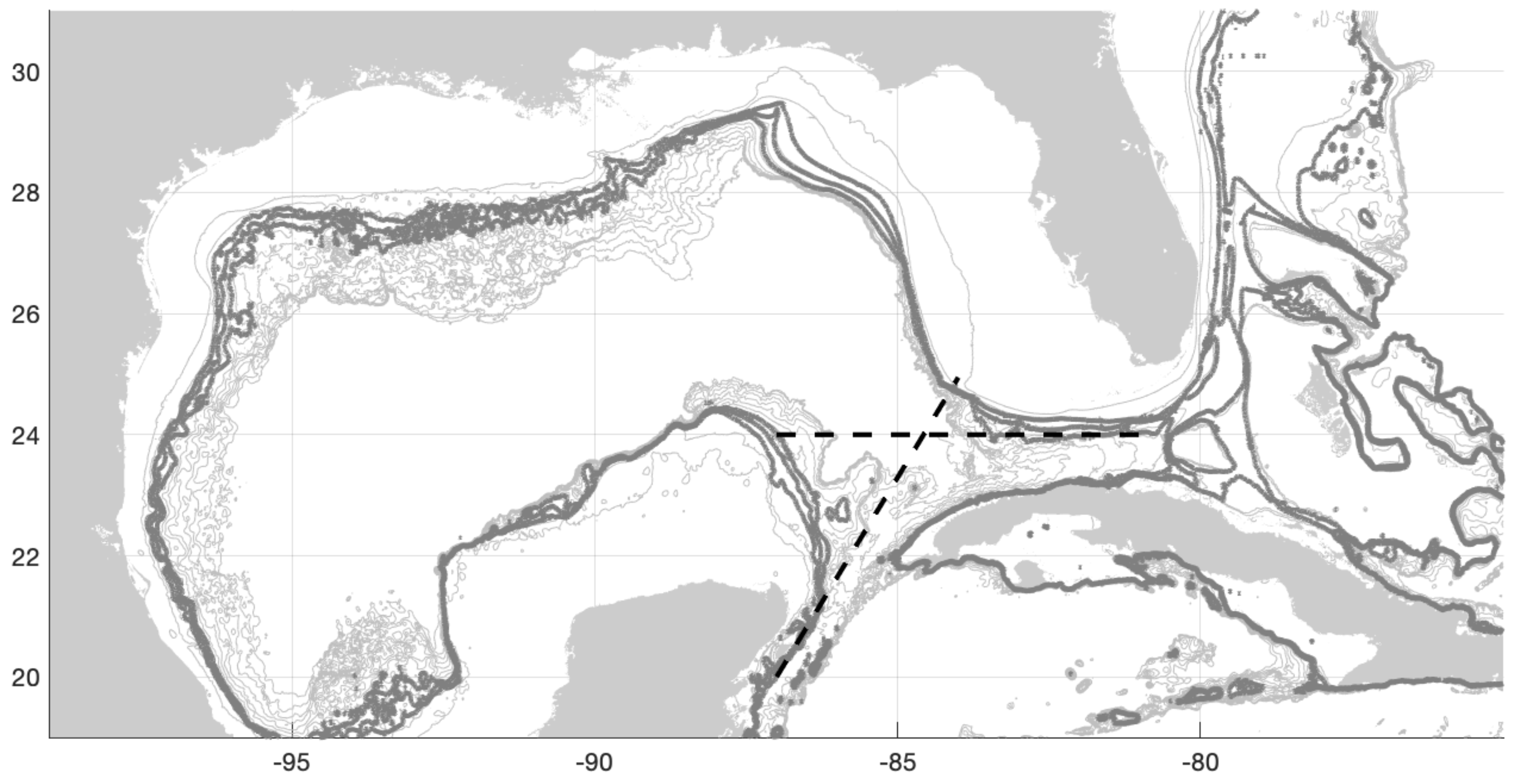
18], the hypothesis has not widely been adopted by the Gulf of Mexico Loop current community. The likely reason for this is the unique geometry of the Gulf of Mexico (Figure 2). Notice that the Yucatan Peninsula has a zonal “offset” from the southern tip of Florida by about 2.5 . Further, the orientation of the boundary current forming along the Yucatan is not parallel to the southern coast of Florida. Instead, the inflowing current makes an approximately 120 degree angle with the outflowing current ( 180 being straight gap with parallel flow). The goal of this manuscript is to show that hysteresis in such gap-leaping western boundary current systems is robust both to gap angle and gap offset.

2. Numerical Model

The numerical model utilized in this study is a barotropic version of the baroclinic model developed and validated in [16,26]. The numerical model was developed to support a series of rotating table laboratory experiments (referenced above). Both the experimental setup and validation of the numerical model have been well-established in the literature, so only a brief summary is provided here. The idealized setup consists of a square tank of width 2 L = 1 m with a sloping bottom to induce a topographic
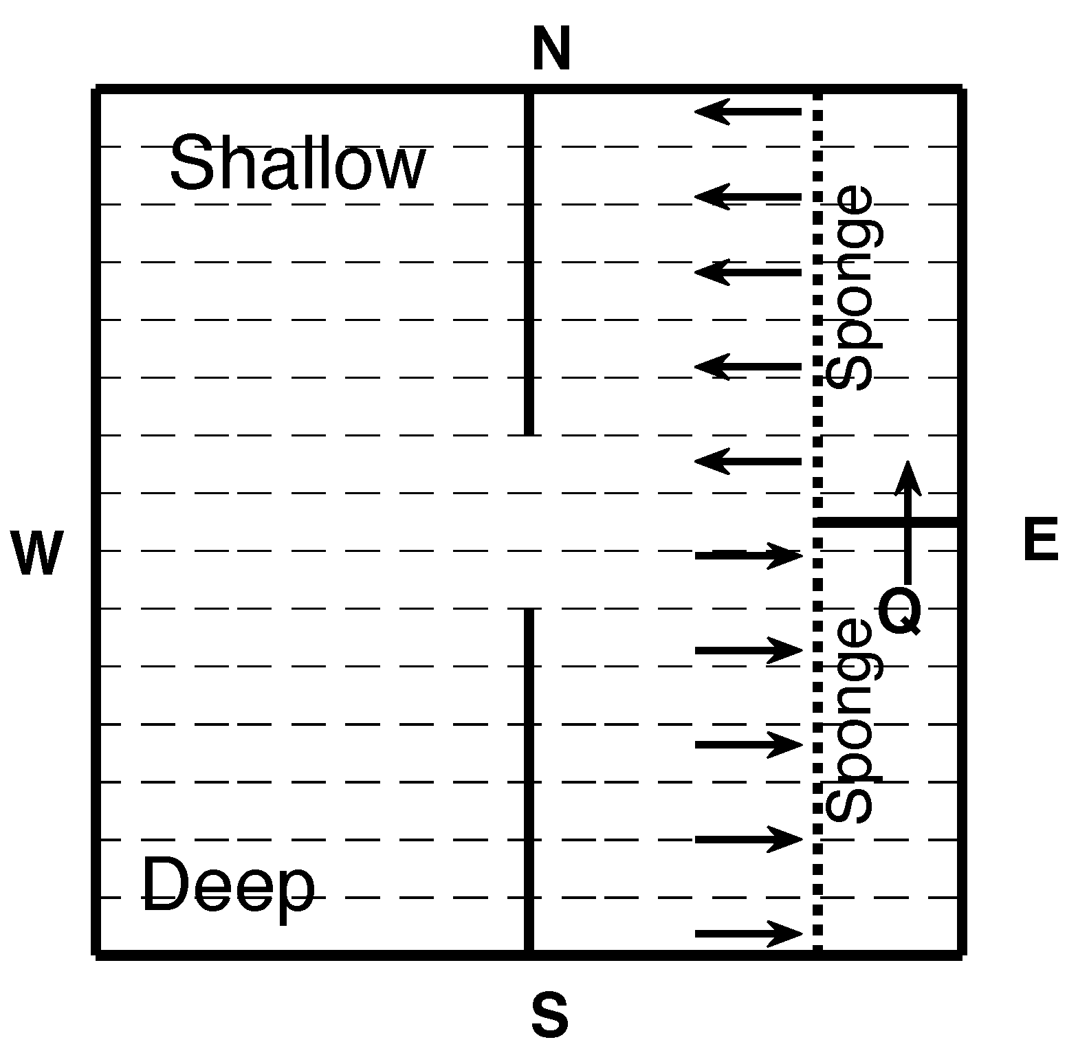
 β -effect. In Figure 3, north corresponds to up and east corresponds to right. The flow is driven by a broad Sverdrup interior circulation from the east, which impinges on a north–south oriented vertical ridge, which extends to the surface, where a predominantly inertial western boundary current forms. Note, in the lab and also in the present model study, it is more convenient to consider a southward flowing western boundary current (flowing from top to bottom in the figures), but, due to the north–south invariance of the quasi-geostrophic barotropic equations, this does not present an issue when interpreting our results in the context of northward-flowing oceanic western boundary currents. The ridge is interrupted at its center by a gap with halfwidth L g = 6 cm, which the western boundary current must negotiate. In the gap region, the western boundary current will either follow geostrophic contours (in this case, constant depth contours) turning into the western basin and forming a loop current or leap directly across the gap. The computations correspond to a mean water depth of H 0 = 20 cm, topographic slope of S = 0.2 (where β = S f / H 0 ), and a table rotation rate of Ω = 0.65 rad/sec (where f = 2 Ω ).
The nondimensional problem is formulated as the potential vorticity advection–diffusion equation, as in the quasi-geostrophic approximation
J ( ψ , q ) + λ S 1 h ω λ M 3 2 ω = 0 ( 1 h ψ ) ω = 0 ,
where ψ is the transport function (defined through the Helmholtz decomposition h u = k ^ × ψ + ϕ with 2 ϕ = 1 2 h E ω representing Ekman divergence), ω = × u is the relative vorticity, and q = ( 1 / β ^ + λ I 2 ω ) / h , h = 1 β ^ y and h E = ν Ω 1 2 is the Ekman depth. The nondimensional parameter β ^ = β L / f = S L / H 0 is the relative meridional variation of depth over the basin due to the sloping bottom, and h is the fluid depth. Our laboratory experiments and numerical model allow for small but finite values of β ^ , while the quasi-geostrophic approximation is the limit of infinitely small β ^ . The domain is 1 < x < 1 , 1 < y < 1 , with north corresponding to positive y and east corresponding to positive x. The kinematic conditions for solving the elliptic equation are ψ = 0 along all boundaries, except at the eastern boundary x = 1 where inflow/outflow is prescribed ψ = Ψ B ( y ) , with Ψ B varying between 0 and 1. The dynamical conditions are no-slip: v = 0 at the western x = 1 , eastern x = 1 boundaries and along the ridge, and no-stress ω = 0 at the southern y = 1 and northern y = 1 boundaries. The “no-slip” is a natural condition of vanishing velocity at a solid boundary. The northern and southern boundaries correspond to the fluid gyre boundaries in the ocean where vorticity and stress are vanishing. In our numerical method, we were restricted by the ridge to be oriented either north–south or diagonally in such a way that the boundary passes through rectangular grid nodes. The values of vorticity at the solid boundaries were calculated assuming the antisymmetry of the tangential velocity component as it was extended outside the fluid domain, which reduces to the formula by Thom [27] for a straight wall. The vorticity values were different on the different sides of the ridge. The arising parameters λ I = U 0 β L 2 , λ S = k 0 β L with k 0 = f ( h E / H 0 ) and λ M = ν β L 3 1 3 are the nondimensional inertial, Stommel, and Munk boundary layer thicknesses as in the standard theory. Where U 0 = Q / ( H L ) is the Sverdrup interior velocity scale, L is the basin length scale, ν is the kinematic viscosity, and Q is the volume flux. With the viscosity of water ν = 0.01 cm 2 /s, for the cases considered here λ M = 0.0183252 , λ S = 0.0124034 , and λ I is varied (typically, λ I = 0.0392232 for Q = 50 cm 3 /s). The corresponding dimensional values (obtained by multiplication by L) were L M = 0.92 cm, L S = 0.62 cm, and L I = 1.96 cm, respectively.
The numerical problem is solved using standard finite differences on a rectangular grid dividing the domain into N x × N y cells. The parameters λ S and λ M represent the dissipative effects, while λ I characterizes the nonlinearity, the strength of the flow. For small boundary layer Reynolds numbers R = ( λ I / λ M ) 3 , simple explicit iterations with treating the nonlinear terms as perturbations work well, but for the moderate R the iterations fail to converge [14]. In this case, Newton’s method has be to employed for finding steady solutions. We consider a state vector X = ( ω , ψ ) consisting of values at all grid nodes including the boundaries, the size of this vector is M = ( N x + 1 ) ( N y + 1 ) 2 . In a symbolic form, the set of Equation (1) is represented by F(X) = 0. Substituting an initial guess X 0 into Equation (1) results in the vector of residuals F ( X 0 ) at each grid node of the same size M. In order to find the next iteration X 1 that brings residual closer to vanishing F ( X ) = 0 , we need to calculate the Jacobian matrix J F [ X 0 ] (of size M × M which depends on X 0 ) of all first-order partial derivatives of F with respect to X and then solve the linear system
J F [ X 0 ] ( X 1 X 0 ) = F ( X 0 )
The iterations then continue until the residual (standard deviation and pointwise error) vanishes to the machine accuracy, O ( 10 11 ) . It usually took about seven or fewer iteration steps to reach such convergence. The elements of the Jacobian matrix can be calculated analytically by considering the variational problem corresponding to Equation (1).
J ( δ ψ , q ) + J ( ψ , δ q ) + λ S 1 h δ ω λ M 3 2 δ ω = 0 ( 1 h δ ψ ) δ ω = 0 ,
where δ q = λ I 2 δ ω / h . The variations of the boundary conditions are trivial. It should be noted that the elements of the Jacobian matrix do not have to be calculated exactly. As long as the iterations converge and the residual F ( X ) vanishes, we get an exact solution to the original problem (1). However, in this idealized problem, we do perform exact analytic calculation of the matrix elements. Finite difference approximations result in a sparse banded type of J F , and the grids of size up to 1000 × 1000 can be solved on a computer with 24 GiB of operational memory.

3. Results

3.1. Angled Gap

We begin by considering the effect of the gap configuration angle. As noted above, the Gulf of Mexico Loop Current encounters an approximately 120 gap angle. Here, we will consider the more extreme configuration of a 90 angle between the ridges forming a gap. This is mainly due to ease of computation. For a 90 configuration, the ridge walls align diagonally with the computational nodes, which facilitates the boundary condition specifications. We note that the existence of hysteresis for a 90 angled gap certainly guarantees the existence of lower gap angle geometries. The resulting hysteresis trace for a L g = 5 cm gap halfwidth at 90 gap angle configuration is shown in Figure 4 in the top two rows.
Starting with lower flow rates and increasing towards higher values (upper panels from left to right in Figure 4A–C), we see the flow is initially in a gap-penetrating flow state with modified β -plumes extending from either gap edge towards the west, roughly following the geostrophic contours [28,29,30,31,32]. As the flow rate increases, the northern β -plume bends further to the south, as the inertia induces the flow to cross isobaths. Eventually, at approximately Q = 59 cm 3 /s, the penetrating state abruptly transitions to a gap-leaping flow state. The system continues to evolve along the gap-leaping solution branch as the flow rate is decreased (the second row of panels from right to left in Figure 4D–F). Eventually, at approximately Q = 33 cm 3 /s, the gap leaping flow state abruptly transitions to a gap-penetrating flow state and the hysteresis loop has been fully traced. In presenting the flow patterns we refer to dimensional values of Q relevant for laboratory experiments. The nondimensional boundary-layer Reynolds number R Q 3 / 2 is also shown in figure panels. The advection dominates the viscous effects when R > 1 .
The configuration with 180 gap configuration angle (essentially a straight ridge) also exhibits multiple states and hysteresis, but the range is smaller between Q = 18–21 cm 3 /s. The extreme gap-penetrating flow at Q = 21 cm 3 /s and gap-leaping flow pattern at Q = 18 cm 3 /s are shown in Figure 4 (third row, two left panels: G, H).
An opposite configuration, when the angle between ridges is 270 , is illustrated in Figure 4 (third row, last two panels). For a weak flow Q = 10 cm 3 /s the β -plume penetrates into the gap. However, as the flow rate increases the pattern soon smoothly changes into a gap leaping state Q = 13 cm 3 /s, and remains such for higher Q. No hysteresis is observed in this smooth transition.
In the 90 angle configuration the upstream current points into the gap, which promotes the penetrating flow pattern: the current only needs to turn 45 in order to enter the gap and become a zonal current in the β -plume region. In the 180 case the upstream current needs to make a sharper turn of 90 in order to enter the gap; therefore, the conditions are less favorable for penetration and the range of hysteresis is smaller. Furthermore, in the 270 angle configuration, the upstream boundary current has to turn 315 in order to enter the gap; therefore, the penetrating flow pattern is not favorable and is easily switched to a gap-leaping pattern as the inertia is increased.

3.2. Offset Gap

Similar to the process described above, a series of hysteresis trace studies were performed for a gap that is formed by two meridional ridges that have not only the meridional separation (halfwidth of L g = 6 cm) but also have a zonal offset, L z , which was varied.
In each case, again, lower flow rates result in penetrating flow states which abruptly transition to leaping flow states as the strength of the western boundary current is increased. Once the system has transitioned to the leaping solution branch, it remains in the leaping states as the strength of the western boundary current is decreased until an abrupt transition back to the penetrating solution branch. The critical flow states can be seen in Figure 5 for a L z = 6 cm negative offset (left panels: A, D); zero-gap offset (middle panels: B, E); a L z = 6 cm positive-gap offset (right panels: C, F). The trend for critical transition states can be seen in Figure 6 with the width of the hysteresis range increasing for positive gap offset and decreasing with negative gap offset. The positive offset corresponds to a configuration that is more favorable for the upstream boundary current to enter the gap if it continued straight forward.

4. Discussion

For the meridional, north–south oriented, ridges without an offset, the mechanism producing the multiple states is intuitively clear: on one hand, the beta-effect (via a potential vorticity gradient across the gap) promotes the boundary current to drift westward and to penetrate through the gap; on the other hand, the meridional advection promotes the current to jump across. Balancing meridional advection and zonal advection against the β -effect lead to two different scaling: Q L g 3 and Q L g (see details in [10]). Hence, two different sets of critical parameter values at which transitions between penetrating and leaping states occur. This is essentially the root cause of hysteresis in such systems. Furthermore, a cusp bifurcation occurs in the parameter space where the two branches coalesce. The cusp is an invariant feature. If instead of varying the gap width as in [10], we vary another parameter that promotes the current penetration (in the present case it is the configuration angle or gap offset), we will recover a similar behavior: the range of hysteresis will vary and disappear when the penetration is sufficiently obstructed. In the angled and offset ridges cases, the upstream boundary current may be directed inside the gap thus promoting the intrusion (gap penetration). So the question is, if we increase the inertia (or transport of the boundary current), will it always promote intrusion?
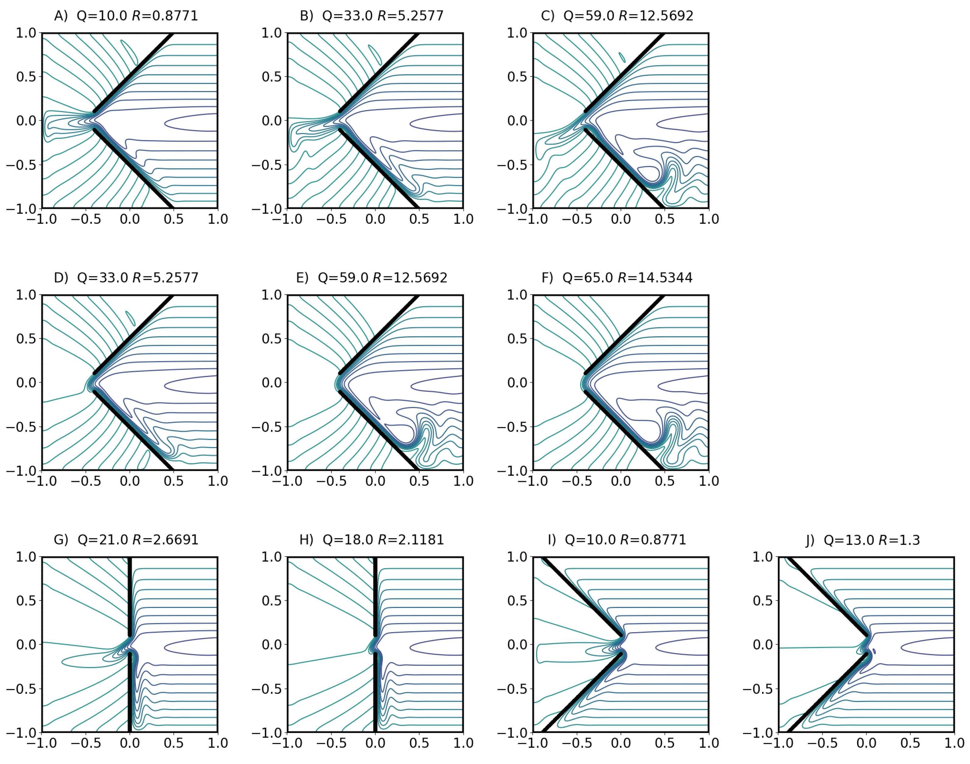
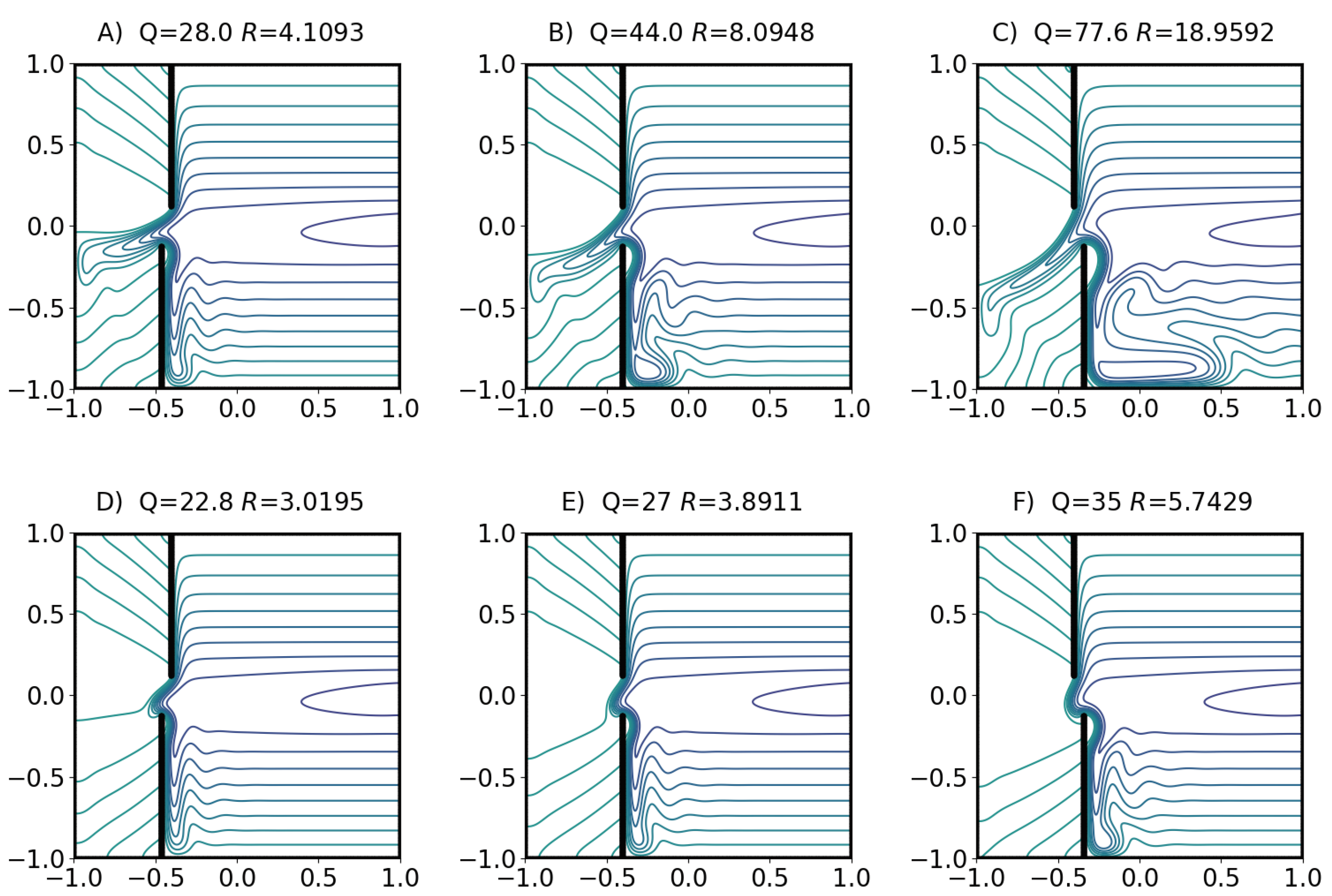
Our previous results (cited above), which are consistent with the findings presented in Figure 4 and Figure 5, have shown that as the width scale of the boundary current, which is a combination of L M , L S , and dominantly L I , exceeds the gap halfwidth, L g , the current ultimately switches to the gap-leaping regime. This apparent contradiction is most easily explained by considering the offset gap results (Figure 5). Increasing the gap offset, L z , with the jet pointing inside the gap (positive offset) will delay this transition compared to the zero offset case, but not prohibit a leaping state. Once the boundary current length scale exceeds the gap halfwidth, a transition occurs. Essentially, as the inertia of the current increases, the boundary layer length scale grows to a point where the current will not be able to squeeze through the gap, and a leaping state will result.
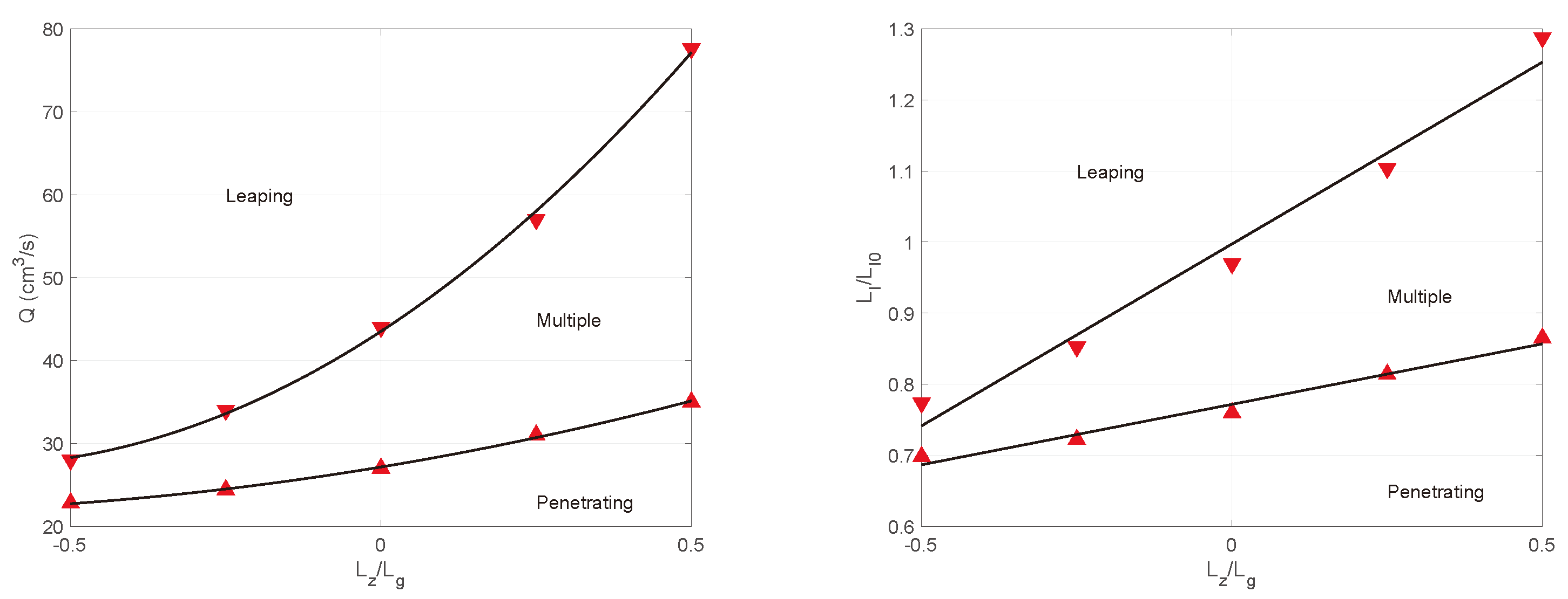
Note the quadratic trend of the leaping to penetrating transitions (Figure 6 upward facing triangles, quadratic trend given by solid curve). The transition condition for a straight gap ( L z = 0 ) scales as the boundary layer length scale becoming comparable to L g . In the case of offset gaps, it is not just the gap halfwidth but also the gap offset must also be accounted. The boundary layers considered are primarily inertial with L I Q . Thus, relative to the straight gap case, we would expect to see a quadratic dependence of critical boundary current transport as a function of L z . This is emphasized by the right panel which shows a near-linear dependence of L I / L I 0 , where L I 0 is the inertial length scale at transition for L z = 0 . Interestingly, the trend for the penetrating to leaping transition behaves similarly.
This also emphasizes the importance of the parameter L I / L g to the penetrating to leaping transition. Or more completely, the ratio of the boundary layer length scale to the gap halfwidth, which is a combination of the Stommel, Munk, and inertial length scale. For typical Gulf of Mexico parameters, the inertial length scale is about 60 km, the Munk length scale is about 30 km, and the Stommel length scale is smaller yet. Thus, typical boundary current length scales would be on the order of 90–100 km. It is also observed that the effective gap halfwidth, between Yucatan and the west Florida shelf, is approximately 150 km. As expected, this puts the Gulf of Mexico Loop Current into a boundary length scale to gap halfwidth ratio parameter regime of around 0.6–0.7, which is consistent with our numerical parameter space. Further, recent results from consideration of realistic Gulf of Mexico topography [20], suggest the Gulf typically operates in an R = 5–15 parameter space, also in agreement with our findings.
The results presented in this manuscript are intended to break the stigma that hysteresis in gap-leaping western boundary current systems only occurs for special geometries (straight gaps with zero offset). Indeed, we have explicitly shown that both angled and offset gap geometries exhibit multiple states and hysteresis. The key insight emphasized in this work is that the more the upstream current is directed into the gap due to geometrical configuration (angled or offset gaps), the more distinct the penetrating and leaping flow patterns are, and the bigger the range of hysteresis in the system is. It should also be noted that the methods utilized in this manuscript have recently been applied to the full-scale Gulf of Mexico [20]. It was found that a barotropic approximation to the upper-layer circulation in the Gulf of Mexico (at full-scale, with a realistic oceanic parameter regime, and for realistic topography similar to Figure 2) displays hysteresis and multiple steady states. Which, given the above results, should be expected.

Author Contributions

J.K. and V.A.S. contributed equally to the analysis, interpretation, and generation of this manuscript. V.A.S. developed the code used in this study. All authors have read and agreed to the published version of the manuscript.

Funding

This research was funded by the National Science Foundation, USA via grant number 1823452 and the National Academies of Sciences, Engineering and Medicine (NASEM) UGOS-1 via grant number 2000009918 and UGOS-2 via grant number 200011071.

Institutional Review Board Statement

Not applicable.

Informed Consent Statement

Not applicable.

Data Availability Statement

The numerical code used in this work can be found at http://sites.udel.edu/kuehl-group/software/ (accessed on 1 January 2022).

Acknowledgments

The authors are thankful to the National Science Foundation, USA for funding this research via grant number 1823452, and to the National Academies of Sciences, Engineering and Medicine (NASEM) UGOS-1 via grant number 2000009918 and UGOS-2 via grant number 200011071.

Conflicts of Interest

The authors declare no conflict of interest. The founding sponsors had no role in the design of the study; in the collection, analyses, or interpretation of data; in the writing of the manuscript, and in the decision to publish the results.

Sample Availability

Not applicable.

References

  1. Committee on Advancing Understanding of Gulf of Mexico Loop Current Dynamics; Gulf Research Program; National Academies of Sciences, Engineering, and Medicine. Understanding and Predicting the Gulf of Mexico Loop Current: Critical Gaps and Recommendations; National Academies Press: Washington, DC, USA, 2018; p. 24823. [Google Scholar] [CrossRef]
  2. Farris, A.; Wimbush, M. Wind-induced Kuroshio intrusion into the South China Sea. J. Oceanogr. 1996, 52, 771–784. [Google Scholar] [CrossRef]
  3. Qiu, B.; Lukas, R. Seasonal and interannual variability of the North Equatorial Current, the Mindanao Current and the Kuroshio along the Pacific western boundary. J. Geophys. Res. 1996, 101, 12315–12330. [Google Scholar] [CrossRef]
  4. Nan, F.; Xue, H.; Xiu, P.; Chai, F.; Shi, M.; Guo, P. Oceanic eddy formation and propagation southwest of Taiwan. J. Geophys. Res. 2011, 116, C12045. [Google Scholar] [CrossRef] [Green Version]
  5. Centurioni, L.R.; Niiler, P.P.; Lee, D. Observations of Inflow of Philippine Sea Surface Water into the South China Sea through the Luzon Strait. J. Phys. Oceanogr. 2004, 34, 113–121. [Google Scholar] [CrossRef]
  6. Wu, C.R.; Hsin, Y.C. The forcing mechanism leading to the Kuroshio intrusion into the South China Sea: Wind-Driven Kuroshio Intrusion. J. Geophys. Res. Oceans 2012, 117, C7. [Google Scholar] [CrossRef] [Green Version]
  7. Hsin, Y.C.; Wu, C.R.; Chao, S.Y. An updated examination of the Luzon Strait transport: Luzon Strait Transport. J. Geophys. Res. Oceans 2012, 117, C3. [Google Scholar] [CrossRef] [Green Version]
  8. Metzger, E.; Hurlburt, H. The nondeterministic nature of the Kuroshio penetration and eddy shedding in the South China Sea. J. Phys. Oceanogr. 2001, 31, 1712–1732. [Google Scholar] [CrossRef]
  9. Yuan, D.; Han, W.; Hu, D. Surface Kuroshio path in the Luzon Strait area derived from satellite remote sensing data. J. Geophys. Res. 2006, 111, C11007. [Google Scholar] [CrossRef] [Green Version]
  10. Sheremet, V.A. Hysteresis of a Western Boundary Current Leaping across a Gap. J. Phys. Oceanogr. 2001, 31, 1247–1259. [Google Scholar] [CrossRef]
  11. Sheremet, V.A.; Kuehl, J. Gap-Leaping Western Boundary Current in a Circular Tank Model. J. Phys. Oceanogr. 2007, 37, 1488–1495. [Google Scholar] [CrossRef]
  12. Kuehl, J.J.; Sheremet, V.A. Identification of a cusp catastrophe in a gap-leaping western boundary current. J. Mar. Res. 2009, 67, 25–42. [Google Scholar] [CrossRef]
  13. Gilmore, R. Catastrophe Theory for Scientist and Engineers; John Wiley and Sons Inc.: Hoboken, NJ, USA, 1981. [Google Scholar]
  14. Sheremet, V.A. A method for finding unstable steady solutions by forward time integration: Relaxation to the running mean. Ocean Model. 2002, 5, 77–89. [Google Scholar] [CrossRef]
  15. Kuehl, J.J.; Sheremet, V.A. Two-layer gap-leaping oceanic boundary currents: Experimental investigation. J. Fluid Mech. 2014, 740, 97–113. [Google Scholar] [CrossRef]
  16. McMahon, C.W.; Kuehl, J.J.; Sheremet, V.A. A Viscous, Two-Layer Western Boundary Current Structure Function. Fluids 2020, 5, 63. [Google Scholar] [CrossRef]
  17. Pichevin, T.; Nof, D. The momentum imbalance paradox. Tellus A 1997, 49, 298–319. [Google Scholar] [CrossRef]
  18. Song, X.; Yuan, D.; Wang, Z. Hysteresis of a periodic or leaking western boundary current flowing by a gap. Acta Oceanol. Sin. 2019, 38, 90–96. [Google Scholar] [CrossRef]
  19. McMahon, C.W.; Kuehl, J.J.; Sheremet, V.A. Dynamics of Gap-leaping Western Boundary Currents with Throughflow Forcing. J. Phys. Oceanogr. 2021. accepted. [Google Scholar] [CrossRef]
  20. Sheremet, V.A.; Kan, A.A.; Kuehl, J. Multiple Equilibrium States of the Loop Current in the Gulf of Mexico. arXiv 2022, arXiv:2111.13810. [Google Scholar]
  21. Wang, Z.; Yuan, D.; Hou, Y. Effect of meridional wind on gap-leaping western boundary current. Chin. J. Oceanol. Limnol. 2010, 28, 354–358. [Google Scholar] [CrossRef]
  22. Mei, H.; Qi, Y.; Qiu, B.; Cheng, X.; Wu, X. Influence of an Island on Hysteresis of a Western Boundary Current Flowing across a Gap. J. Phys. Oceanogr. 2019, 49, 1353–1366. [Google Scholar] [CrossRef]
  23. Yuan, D.; Wang, Z. Hysteresis and Dynamics of a Western Boundary Current Flowing by a Gap Forced by Impingement of Mesoscale Eddies. J. Phys. Oceanogr. 2011, 41, 878–888. [Google Scholar] [CrossRef]
  24. Lien, R.C.; Ma, B.; Cheng, Y.H.; Ho, C.R.; Qiu, Q.; Lee, C.M.; Chang, M.H. Modulation of the Kuroshio transport by mesoscale eddies at the Luzon Strait entrance. J. Geophys. Res. Oceans 2014, 119, 2129–2142. [Google Scholar] [CrossRef]
  25. Yuan, D.; Song, X.; Yang, Y.; Dewar, W.K. Dynamics of Mesoscale Eddies Interacting with a Western Boundary Current Flowing by a Gap. J. Geophys. Res. Oceans 2019, 124, 4117–4132. [Google Scholar] [CrossRef]
  26. McMahon, C.W.; Kuehl, J.J.; Sheremet, V.A. On the Dynamics of Gap-Traversing Western Boundary Currents with Throughflow Forcing. J. Phys. Oceanogr. 2020. accepted. [Google Scholar]
  27. Thom, A. The flow past circular cylinders at low speeds. Proc. R. Soc. Lond. A 1933, 141, 651–669. [Google Scholar]
  28. Gill, A.E.; Smith, R.K. On similarity solutions of the differential equation Ψzzzz + Ψx = 0. Proc. Camb. Philos. Soc. 1970, 67, 163–171. [Google Scholar] [CrossRef]
  29. Cleary, S.P. A Generalized Heat Equation. Ph.D. Thesis, Department of Mathematics, Michigan Technological University, Houghton, MI, USA, 1987; 33p. [Google Scholar]
  30. Ibanez, R.; Kuehl, J.; Shrestha, K.; Anderson, W. Brief communication: A nonlinear self-similar solution to barotropic flow over varying topography. Nonlinear Process. Geophys. 2018, 25, 1–17. [Google Scholar] [CrossRef] [Green Version]
  31. Kuehl, J.J. An analytic solution for barotropic flow along a variable slope topography. Geophys. Res. Lett. 2014, 41, 7591–7594. [Google Scholar] [CrossRef]
  32. Kuehl, J.; McMahon, C. An analytic solution for bottom intensified flow along sloping topography. Eur. J. Mech.- B/Fluids 2020, 82, 156–160. [Google Scholar] [CrossRef]
Figure 1. Gulf of Mexico topography with light grey indicating isobaths 5:100:3500 m and dark grey indicating isobaths 250, 500, 1000, and 2000 m. Grey mask indicates land. Superimposed are sea surface height contours for: (Left) on and around the 193rd day of 2015. (Right) on and around the 57th day of 2017.
Fluids 07 00071 g001
Figure 2. Gulf of Mexico topography with light grey indicating isobaths and dark grey contours indicating the slope. Grey mask indicates land. Dashed lines extend regions of slope against which boundary currents flow. Notice that the Yucatan Peninsula has a zonal “offset” from the southern tip of Florida by about 2.5 . Further, the orientation of the boundary current forming along the Yucatan is not parallel to the southern coast of Florida. Instead, the inflowing current makes an approximately 120 degree angle with the outflowing current ( 180 being a straight gap with parallel flow).
Fluids 07 00071 g002
Figure 3. Top view of the numerical/tank setup. Constant depth contours are indicated by dashed lines. The transport, Q, drives the interior circulation.
Fluids 07 00071 g003
Figure 4. Hysteresis trace for various angled gap configurations of western boundary current, gap halfwidth L g = 5 cm. Shown are the transport functions with contour interval 0.1 . Two upper rows are for 90 configuration: from left to right, the top row (panels AC) shows the transport function for gap-penetrating states for increasing transport, Q; from right to left, the second row (panels DF) shows the transport function in leaping states for decreasing transport. Note the presence of multiple steady flow states between Q = 33 59 cm 3 /s (panels BE). The third lowest row shows (first two panels: G,H) 180 configuration (straight ridge) Q = 21 cm 3 /s gap-penetrating and Q = 18 cm 3 /s gap-penetrating state, with multiple states possible between Q = 18–21 cm 3 /s. The last two panels in the third row (I,J) illustrate smooth (without hysteresis) flow pattern transition for 270 gap configuration as the flow rate varies.
Fluids 07 00071 g004
Figure 5. Shown are the critical flow states (transport function) for: (left panels: A,D) −6 cm gap offset; (middle panels: B,E) zero gap offset; (right panels: C,F) 6 cm gap offset. Contour interval is 0.1. Upper panels show increasing flow rates, while lower panels show decreasing flow rates.
Fluids 07 00071 g005
Figure 6. Critical transition transport values as a function of gap offset. Downward triangles indicate the penetrating to leaping transition. Upward triangles indicate the leaping to penetrating transition. Left Panel: Dimensional transport with black curves representing quadratic fits. Right panel: L I / L I 0 with black curves representing linear fits.
Fluids 07 00071 g006
Publisher’s Note: MDPI stays neutral with regard to jurisdictional claims in published maps and institutional affiliations.

