The Influence of Exit Nozzle Geometry on Sweeping Jet Actuator Performance

Abstract

When pressurized with a fluid, the sweeping jet actuator (SWJA) emits a self-induced and self-sustained temporally continuous, but spatially oscillating bi-stable jet at the outlet. The SWJA adds up local momentum using the Coanda extension without any moving parts and, therefore, can be a promising tool for suppressing aerodynamic flow separation. However, the SWJA needs to be integrated into curved aerodynamic surfaces with an angle. The present study focuses on investigating the effects of various exit nozzle geometries on the flow field. The geometric parameters considered were the exit nozzle angle, diffuser arm length, and curvature. The working fluid was air, and the mass flow rate was 0.015 lb/s. A set of time-dependent flow fields was computed using a two-dimensional unsteady Reynolds-averaged Navier–Stokes (URANS) simulation. The time history of pressure was recorded inside the upper and lower feedback channels. The jet oscillation frequency was obtained by employing the fast Fourier transform (FFT) for all datasets. The results were compared against the baseline case and data available in the literature. The results showed that external geometric variations at the nozzle exit had a negligible impact on the oscillation frequency. However, there were notable effects on the pressure and velocity distribution in the flow field, indicating that the actuator had sensitivity towards the geometric variation of the exit nozzle—the wider the exit nozzle, the lower the downstream velocity. Notably, we observed that the mean velocity at the exit nozzle downstream for the curvature case was 40.3% higher than the reference SWJA.

1. Introduction

The fluidic oscillator has been studied experimentally earlier to understand the model better, as well as contribute to developing the numerical setup. Cattafesta [1] provided an overview of actuators including classification, as well as the working principle of this transducer through controlling the electric signals to avoid disturbance and improving the control mechanism. The preliminary design of a fluidic oscillator contains two different inlets through which fluids enter into the mixing chamber to create the oscillating frequency. This type of oscillator is termed the “feedback-free oscillator”, and Tomac et al. worked on observing the performance of the fluidic oscillator due to dimensional variation to check the optimal operating range [2]. The result showed a fluctuating behavior of the oscillator with the change of the aspect ratio, size, and fluid type. The extension of this work experimented with the performance of the fluidic oscillator at a lower flow rate (below 3.4 mL/s) [3]. The result showed that both of the jets bifurcated each other without completely cutting off. Raghu et al. [4] focused on different methods to produce sweeping jets along with frequencies and flow rates starting from the history. The fluidic oscillator with feedback channels with a single inlet and two different outlets for producing a pulsing jet was also discussed, which is known as the “angled oscillator”. In Kara et al. [5], a numerical model was developed for analyzing the efficiency of SWJA to control the flow separation through active flow control. A two-dimensional (2D) unsteady Reynold’s-averaged Navier–Stokes (URANS) model was used in a wall-mounted hump model with the actuator integrated in an inclined direction. Moreover, the computational fluid dynamics (CFD) simulation extended the future possibility of the three-dimensional (3D) analysis of the hump model. Another article [6] by Kara et al. based on the 3D model of URANS analyzed the internal and external flow over a variety of mass flow rates and determined the pressure drop and the effect on the jet oscillation. The computational analysis was validated with several experimental and numerically proven data by varying the geometry, type and the working fluid accordingly. A computational study for the characterization of the jet oscillation of the actuator was conducted by Furkan et al. [7] by varying the mass flow rate from incompressible to subsonic compressible flow. This 3D URANS model with a stable mesh structure was proven to be a cost-effective alternative for SWJA performance analysis. A notable finding was the constant Strouhal number (implying a stable oscillating flow mechanism) for the oscillating jet. Variation of the inlet mass flow rate was considered to analyze the flow characteristics of the SWJA along with the pressure drop, velocity magnitude, and the formation of vorticity by Kara et al. [8]. Koklu et al. [9] experimentally analyzed how the Coanda extension at the exit nozzle can contribute to the actuator’s flow control capability in a wind tunnel. The actuation with the Coanda extension was then applied to the advance pressure gradient (APG) ramp model, and the performances of the actuator on both models were then compared. A parametric extension by Koklu [10] was also conducted on the efficacy of controlling the flow separation with the SWJA where geometric constraints were elaborately explained. A recent article by Aram et al. [11] explained the interaction of the SWJA with attached turbulent cross-flow using an improved delayed detached-eddy simulation (DDES) model. Bohan et al. [12] performed an excellent analysis of the oscillation frequency and oscillatory spread angle variation caused by the oscillator scale and working fluid.

An experimental investigation was performed using an optimized schlieren. It was combined with a high-speed camera to visualize and investigate the internal dynamics of the SWJA using the Fourier transformation, phase information, and the Hilbert transformation [13]. Ott et al. tried to find the time–space interface of SWJAs for high sweeping frequencies [14]. Another approach to the design optimization of the SWJA to increase the peak jet velocity output and pressure drop reduction was carried out by Jeong [15]. The Boeing 757 vertical tail [16], which contains 37 SWJAs, was tested under nominal airspeed (100 kn), and the best possible situation using 12 SWJAs was found, under the no-slip condition through a significant increase in the suction pressure and side force. Park experimentally investigated the thermal properties(Convective heat transfer-Nusselt Number) and flow distribution of sweeping jet impingement on a flat wall [17]. Pack experimented in a subsonic channel and found that an AFC-controlled high-lift system can reduce the excessive drag force and vehicle weight, thereby saving on the fuel cost [18]. Experimental analysis by Ostermann et al. [19] explained the time-resolved flow field created by a fluidic actuator on a spatially oscillating jet by changing different parameters such as the velocity ratio, installation angle, and Strouhal number. Another experimental analysis [20] was carried out by Park et al. to investigate the effect of the internal geometric parameters of the oscillators on the sweeping jet oscillation distribution.

The present study is a discussion on the geometric variation of the exit nozzle to understand the flexibility of its installation in a complex system. Moreover, this analysis gives a direction for improving the actuator design effectively in the future.

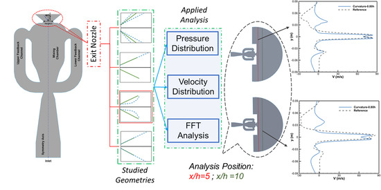
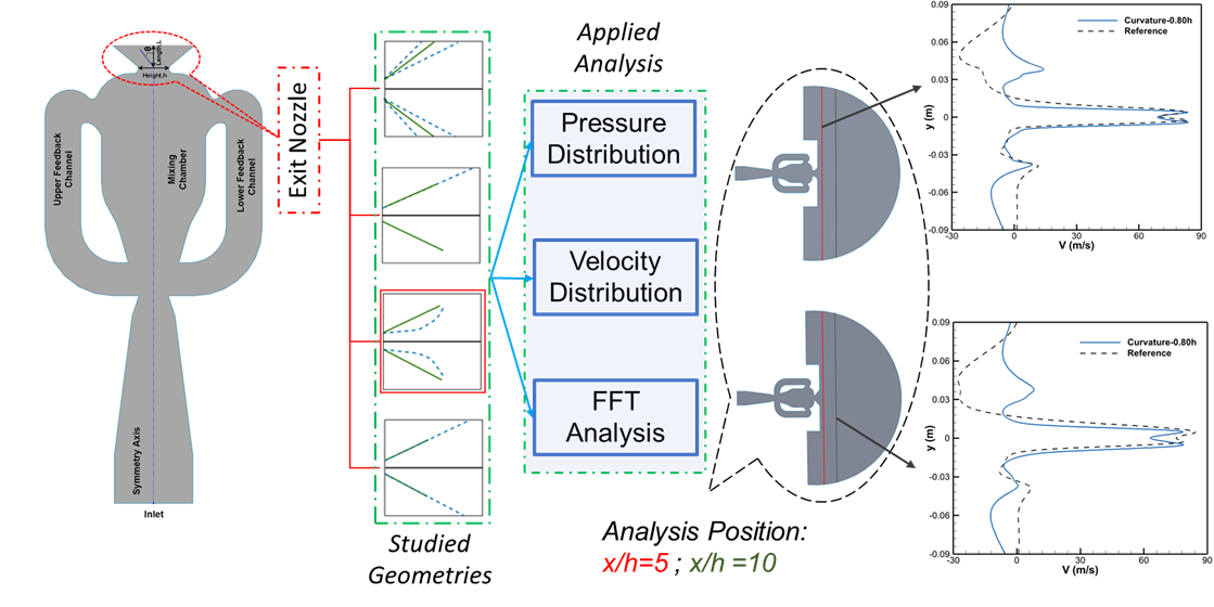
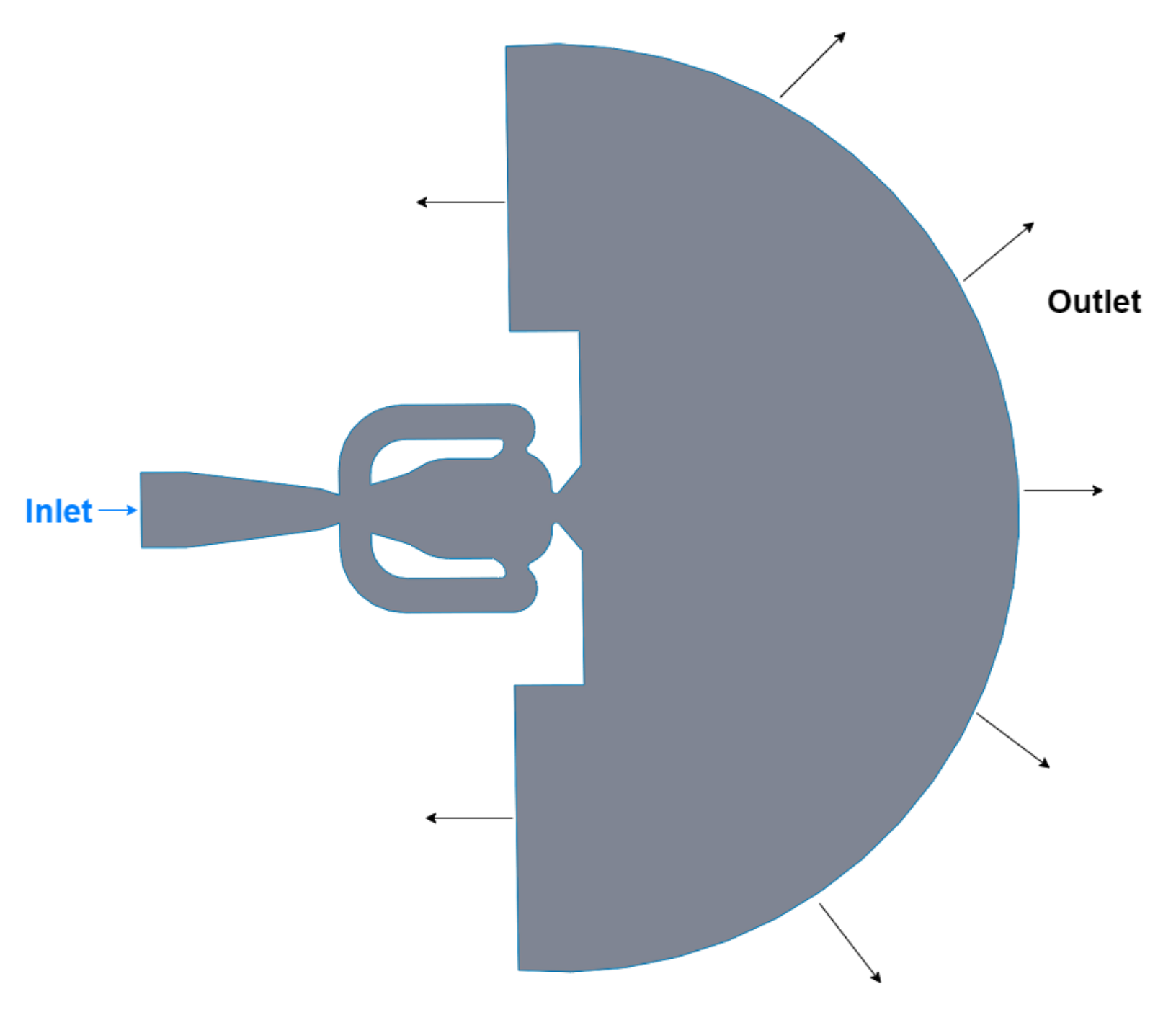
2. Numerical Setup and Geometric Details

The baseline geometry considered for the present study was a curved SWJA having two feedback channels, a mixing chamber, and an exit nozzle [5,6,7,8]. The baseline CAD geometry can be shared upon request. The actuator performance was studied in a quiescent environment with an extended parabolic flow domain downstream of the exit nozzle (Figure 1). The actuator nozzle throat height was h = 6.35 mm. We studied four different shapes of the exit nozzle, namely angle, L-top, L-both, and curvature (Figure 2). For our angle case, we changed the exit nozzle angle from 70${}^{°}$ to 130${}^{°}$ with an increment of 10${}^{°}$ gradually to observe the frequency and variation in the flow distribution. For the curvature case, it was the nozzle length. We varied the exit nozzle length from 0.70 h to 1.30 h with 0.10 h increments and correspondingly changed the curvature radius. We created the arc by keeping the tangent with the base (nozzle length) and normal. Similarly, nozzle length variation was adopted with 0.10 h increments (for our baseline case, the nozzle length was 0.86 h) for the L-top and L-both cases. The only difference was in L-top: the top arm length was adjusted based on the nozzle length, and the other arm was kept constant as the baseline (0.86 h); for the L-both case, both nozzle arms were varied.

3. Governing Equations

The present study required a time-based solver model for a single-inlet mass flow (as mass flux) for which unsteady Reynold’s-averaged Navier–Stokes (URANS) equations for mass continuity, momentum, and energy conservation were considered [6] and the shear stress transport (SST) k-$\omega$ model was chosen for turbulence closure. We studied a single mass flux (J = 66.12 kg/m${}^2$s) (inlet Mach number, M${}_i$ = 0.16 < 0.3) at the subsonic level, but fully turbulent compressible flow was considered since the variation of the Mach number exceeded 0.3 at the exit nozzle throat (maximum Mach number, M${}_{max}$ = 0.627 > 0.3) [21,22,23].

The governing equations are given below:

Continuity equation:

$$\frac{\partial \overline{\rho }}{\partial t}+\frac{\partial \left(\overline{\rho }{\overline{u}}_i\right)}{\partial x_i}=0$$

(1)

Here, $x_i$ are the spatial coordinates and $u_i$ is the velocity components, and since it is an unsteady analysis ($\overline{\rho }$), density is a function of time.

Momentum equation:

$$\frac{\partial \left(\overline{\rho }\overline{u_i}\right)}{\partial t}+\frac{\partial \left(\overline{\rho u_i{u}_j}\right)}{\partial x_j}=-\frac{\partial \overline{P}}{\partial x_i}+\frac{\partial [2{\overline{\nu }}_T\overline{S_{ij}}-\overline{\rho u_i^{″}{u}_j^{″}}]}{\partial x_j}$$

(2)

Here, ${\nu }_T$ is the kinematic eddy viscosity and $S_{ij}$ the mean strain-rate tensor, and pressure $\overline{P}$ was obtained from the ideal gas law. Energy equation:

$$\begin{array}{cc}\hfill \frac{\partial }{\partial t}[\rho (\overline{e}+\frac{\overline{u_i}\overline{u_i}}{2})+\frac{\left(\overline{\rho }\overline{u_i^{″}}\overline{u_i^{″}}\right)}{2}]+& \frac{\partial }{\partial x_j}[\overline{\rho }\overline{u_j}(\overline{h}+\frac{{\overline{u}}_i{\overline{u}}_i}{2})+{\overline{u}}_j\frac{\overline{\rho u_i^{″}{u}_i^{″}}}{2}]=\frac{\partial }{\partial x_j}[-q_{L_j}-\overline{\rho u_j^{″}{h}^{″}}+\overline{t_{j}i{u}_i^{″}}\hfill \\ \hfill & -\overline{\rho u_j^{″}\frac{1}{2}{u}_i^{″}{u}_i^{″}}]+\frac{\partial }{\partial x_j}\left[u_i(2{\overline{\nu }}_T\overline{S_{ij}}-\overline{\rho u_i^{″}{u}_j^{″}})\right]\hfill \end{array}$$

(3)

where $\overline{e}$ is the specific internal energy and $\overline{h}$ the specific enthalpy, and $q_L$ was determined using Fourier’s law of conduction. The working fluid considered here was air with the consideration of the ideal gas density ${\rho }_{in}$ = 1.183 kg/s, and the molecular viscosity was taken based on the three-coefficient method of Sutherland’s law:

$${\mu }_T=\mu {\frac{T}{To}}^{3/2}\frac{(To+S)}{(T+S)}$$

(4)

where the reference viscosity ${\mu }_o$ = 1.716 × 10${}^{-5}$ kg/(ms), reference temperature $T_{ref}$ = 273.16 K, and effective temperature S = 110.56 K, and the reference static pressure was taken as atmospheric pressure (=101,325 Pa).

Computational Fluid Dynamics Model

The flow regime was assumed as fully turbulent for which the SST k-w model was chosen among the RANS models along with the continuity, momentum, and energy equation. The coupled scheme with second-order accuracy was used for solving the pressure, momentum, kinetic energy, and dissipation rate. The turbulence effect was combined using the standard two-equation kinetic energy, k, and energy dissipation, $\omega$, with the shear stress transport constraint making this model suitable for our study.

The second-order discretization was used for pressure, and the second-order upwind formulation was used for the density, momentum, turbulent kinetic energy, specific dissipation rate, and energy. For time-accurate simulation, the bounded second-order implicit scheme was adopted. The residual for the transport equations was considered up to 10${}^{-6}$.

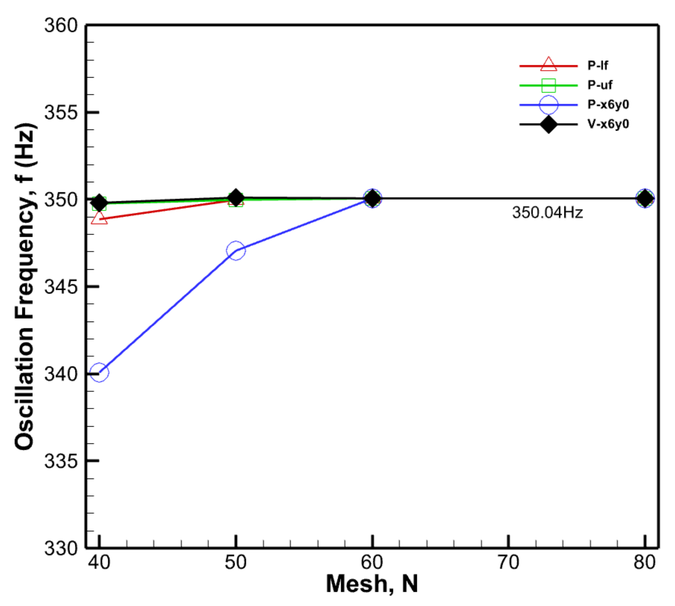
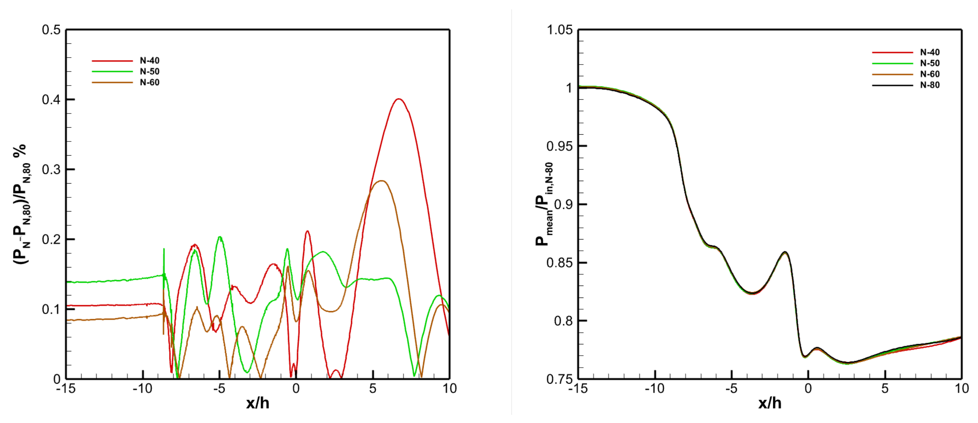
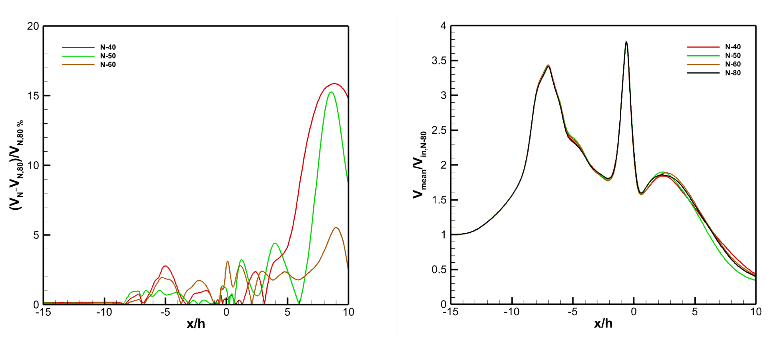
4. Mesh Independence Test

The internal geometry of the sweeping jet actuator has a complex flow physics, and to capture the accurate flow pattern, the flow domain for computation needs to be very precise. To optimize the truncation and round-off error and validate the discretized domain for unsteady simulation, a mesh independence test was required. For the present study, four different (2D) surface meshes were produced considering the exit nozzle height (h = 6.35 mm) as a critical parameter. CFD fluent meshing was performed using ANSYS-2020. The mesh names were based on the element size, which was a function of the characteristic length, h. SST k-$\omega$ was used for turbulent closure. Wall Y+ was kept less than one to resolve the actuator boundary. Ten layers were used near the actuator wall with the first layer thickness h/500 = 0.0127 mm. The details of the tested mesh can be found in

Table 1. Mesh details for computation.

Mesh Name	Total Number of Elements	Total Number of Nodes
N-40	199,489	201,155
N-50	288,969	290,932
N-60	397,342	399,634
N-80	1,008,947	1,012,880

. The final mesh chosen for simulation was N-60, which contained 396,973 quadrilateral and 369 triangular elements with a maximum skewness of 0.71889. Therefore, N-60 indicates that the number of elements along the exit nozzle is 60 and the element size is h/60. Similarly, N-40, N-50, and N-80 have element sizes of h/40, h/50, and h/80, respectively. For a gradual increment of the element size, two spheres of influence were used having radii of 7.5 h and 20 h with a growth rate of 1.15 [6,7]. The mesh name was based on the element size chosen for the smaller sphere, but for the entire structure, the element size was controlled by keeping a tenth of the characteristic length (N-10) (Figure 3), except for N-80, which was considered to be exact, so we used an element size of N-40 for the entire flow domain.

Figure 4 shows the sampling data at three different locations for 0.02 s. Based on the pressure signals, fast Fourier transform (FFT) analysis was conducted, which converts the signal into the frequency domain and captures the peak to determine the oscillation frequency of the system. The computational setup was stabilized using 10,000 time steps with a step size of 1 × 10${}^{-5}$ s, and after that, data sampling analysis was performed on bi-stable oscillation for 0.1 s with the same step size. A pressure-based solver setup was used with a velocity inlet of 55.8 m/s, which corresponds to a mass flow rate of 6.8 g/s, and the ambient pressure outlet condition was considered. Eventually, further analysis on the diffuser was performed using the same mass flow rate. The mesh independence test was performed on the baseline geometry [5].

FFT analysis results showed that the oscillation frequency from mesh N-60 was stable for the actuator. Pressure sampling can provide better signals for the power spectral density (Figure 5). In addition, time-averaged analysis was performed on the mean pressure and velocity along the centerline for the various mesh setups and using MATLAB; local error analysis was conducted using cubic spline interpolation on N-80 to match the number of data points for each mesh setup. From Figure 6 and Figure 7, we can observe that the N-60 mesh distribution was quite reasonable to capture the flow distribution (the maximum error was 5.5%). Therefore, based on both the time-averaged and unsteady results, N-60 was chosen for further analysis.

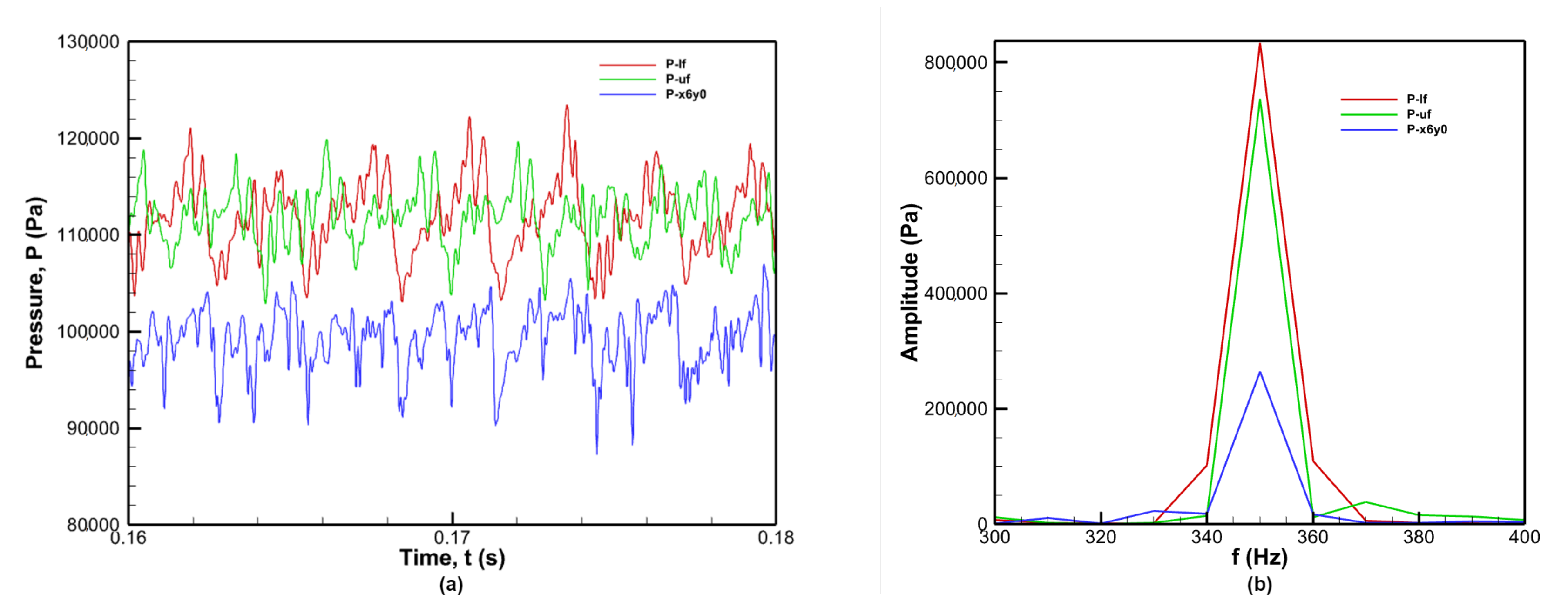
5. Model Validation and Verification

The present study was based on a single mass flow rate (=6.8 g/s) in terms of the mass flux as the inlet condition, and we compared both the numerical and experimental data including the oscillatory frequency and Strouhal number for the corresponding mass flow rate. As our data included both validation and verification for our case, they gave a strong foundation to our model for the further case study.

Table 2. Model validation and verification.

Ref.	Analysis Type	Strouhal Number	Oscillatory Frequency	Error
Slupski [24]	Experimental	0.0160	337.70 Hz	-
Furkan [7]	Numerical (3D-URANS)	0.0131	341.80 Hz	1.21%
Present Study	Numerical (2D-URANS)	0.0134	350.04 Hz	3.64%

shows that the 2D numerical model can determine the oscillatory frequency quite well compared to the 3D model in terms of error % obtained from the experimental result [24]. The Strouhal number also showed a very good agreement with the 3D simulation [7].

6. Results and Discussion

The sweeping jet actuator is an active flow control device having a diffuser, mixing chamber, and feedback channel, and it produces a bi-stable spanwise oscillation at the downstream exit nozzle. The computational setup for this study was similar to the mesh independence test. The geometric modifications were based on the critical dimension; the exit nozzle throat and the variation of the parameters were analyzed after that location. Based on the mean velocity ratio ($\eta \%=V_{case}/V_{Baseline}*100$) obtained at a downstream (x/h = 5) location, we evaluated the efficiency of the respective geometry [7,25]. The red color in the error bars indicates an efficiency lower than the baseline, where the blue bars are the baseline and the green bars show an efficiency higher than the baseline case. The FFT was performed at the upper and lower feedback channel since these locations were consistent for all the geometries.

Table 3. Oscillation frequency for different cases at the upper and lower feedback channel.

Curvature
Sampling Points	0.86 h *	0.70 h	0.80 h	0.90 h	1.00 h	1.10 h	1.20 h	1.30 h
P-lf (Hz)	350.04	348.03	349.84	349.96	349.97	360.91	360.03	360.98
P-uf (Hz)	350.01	349.16	350.09	349.91	349.96	360.03	360.96	360.10
Angle
Sampling Points	35 deg	40 deg	45 deg	50 deg *	55 deg	60 deg	65 deg
P-lf (Hz)	359.03	359.03	359.84	350.04	350.05	339.98	339.98
P-uf (Hz)	359.96	359.54	359.93	350.01	350.28	340.23	340.10
L-top
Sampling Points	0.86 h *	0.70 h	0.80 h	0.90 h	1.10 h	1.20 h	1.30 h	1.50 h
P-lf (Hz)	350.04	339.98	350.16	350.03	350.24	349.91	350.03	350.43
P-uf (Hz)	350.01	340.10	350.13	350.40	350.03	349.90	350.17	349.96
L-both
Sampling Points	0.70 h	0.80 h	0.86 h *	1.10 h	1.20 h	1.30 h
P-lf (Hz)	340.11	340.91	350.04	349.97	350.03	359.84
P-uf (Hz)	339.91	339.98	350.01	350.42	350.17	359.16

* Baseline; P-lf, pressure sampling data at the lower feedback channel; P-uf, pressure sampling data at the upper feedback channel.

manifests the oscillation frequency for each case based on pressure sampling. The mean pressure and velocity distribution at the centerline were obtained from the time average of instantaneous velocity and pressure for 0.1 s. The half-jet width was measured at the x/h = 5 location for all the cases. It was defined as the distance between two points where the peak means the velocity drops by half. The half-jet width indicates the jet spreading downstream influenced by the exit nozzle [25]. Since the curvature cases showed the most promising results, instantaneous total pressure at the centerline was studied to analyze the pressure drop downstream.

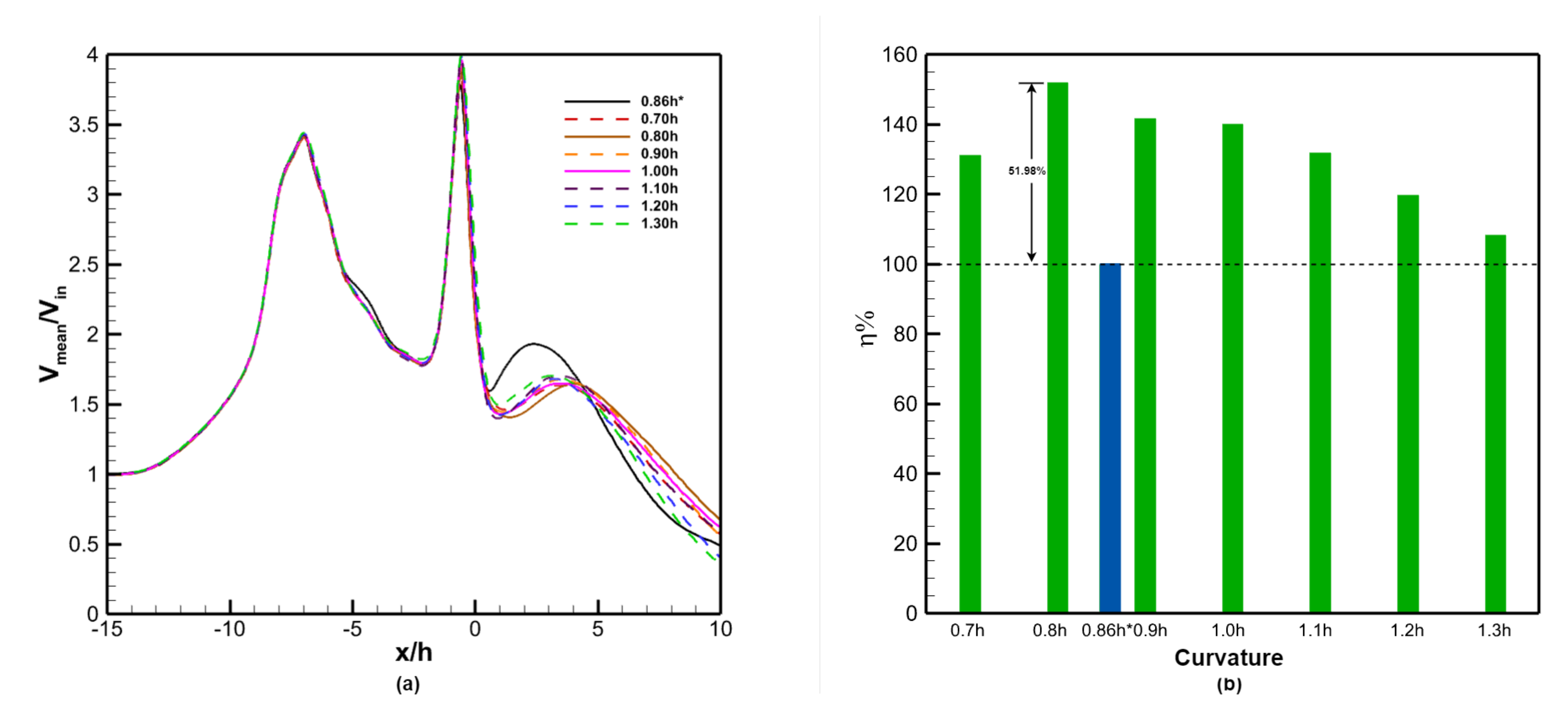
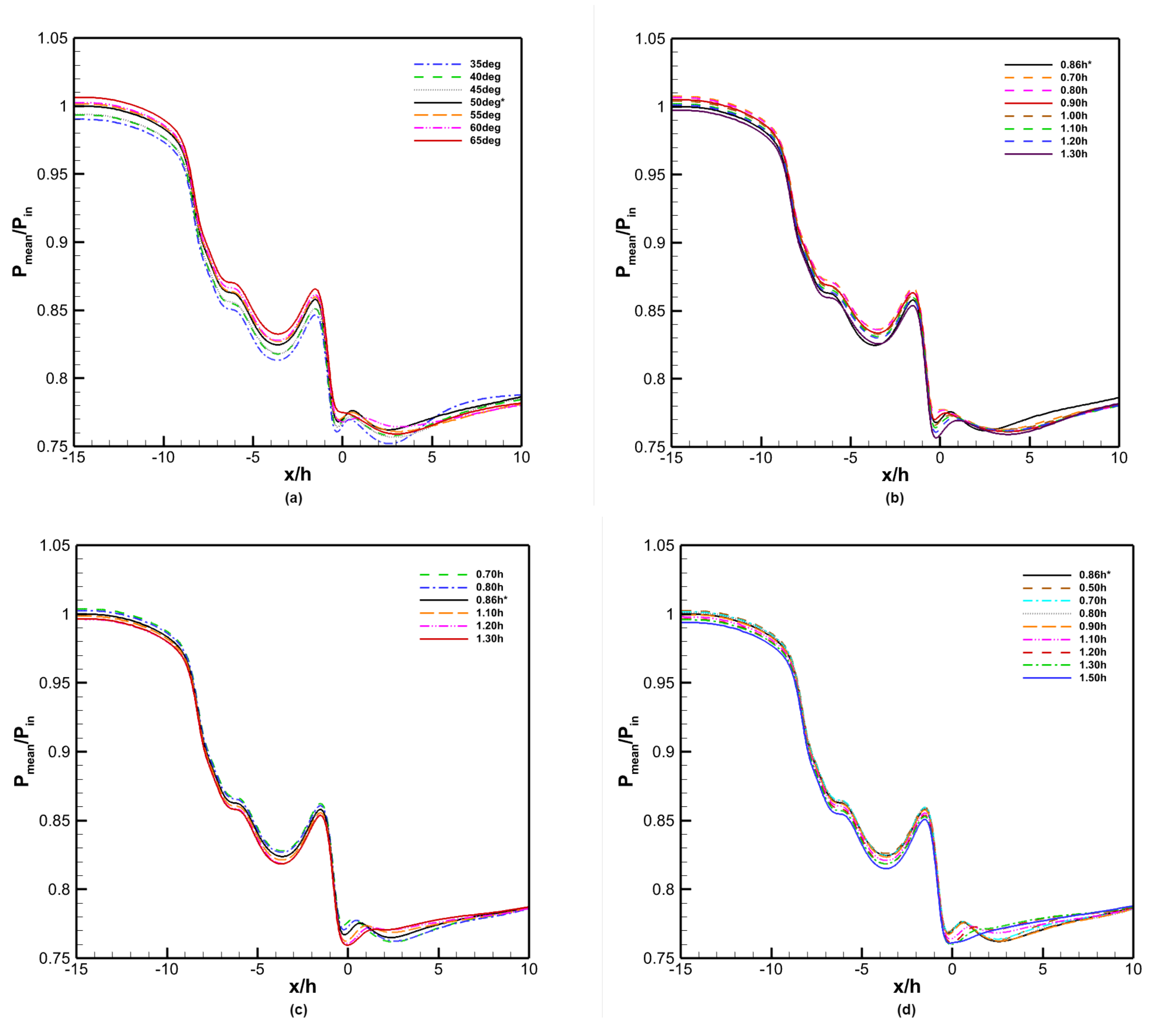
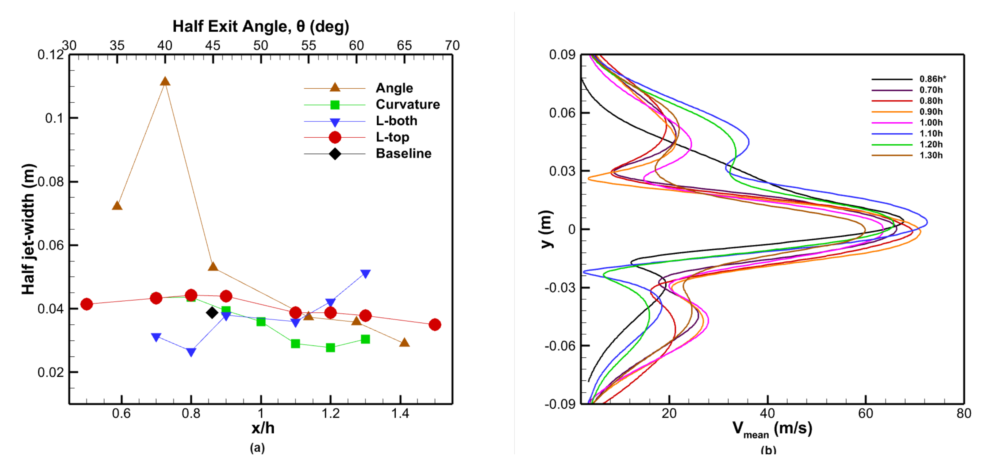
6.1. Effect of Curvature

The nozzle exit length varied from 0.70 h to 1.30 h with 0.10 h increments, and the curvature radius changed accordingly. Compared to the straight nozzle exit (baseline), the curved nozzle exit caused higher dispersion in the velocity (Figure 8). Because of the Coanda effect, the jet tended to adhere to the curved nozzle exit surface, causing the uniform distribution of velocity at the exit nozzle. Compared to the baseline case where the higher velocity was observed after the exit nozzle and then suddenly dropped from x/h = 5, the curvature resulted in a higher mean velocity downstream. The velocity ratio at point x/h = 5 showed that the efficiency could be increased as much as 51.98% (0.80 h) compared to the baseline case. The instantaneous velocity contour plot for the extreme cases (0.70 h and 1.30 h) can be found in the Supplementary Materials. As expected, Figure 9b depicts the gradual reduction of the pressure at the downstream exit nozzle for the curvature cases, following the same pattern as the velocity. In addition, the instantaneous pressure showed an overall pressure drop at the downstream location, influenced by the curvature radius (Figure 10). Finally (Figure 11b) shows that the oscillation downstream was uniform and symmetric for all the cases along with the baseline. In the FFT analysis (Table 3), the magnitude of the oscillation frequency varied within 10.94 Hz compared to the baseline case. However, it followed a trend with the shortest length (0.70 h) having a lower frequency (348.03 Hz) and the maximum length (1.30 h) having the highest frequency (360.98 Hz), while the frequency changed as much as 10 Hz between 1.00 h and 1.10 h.

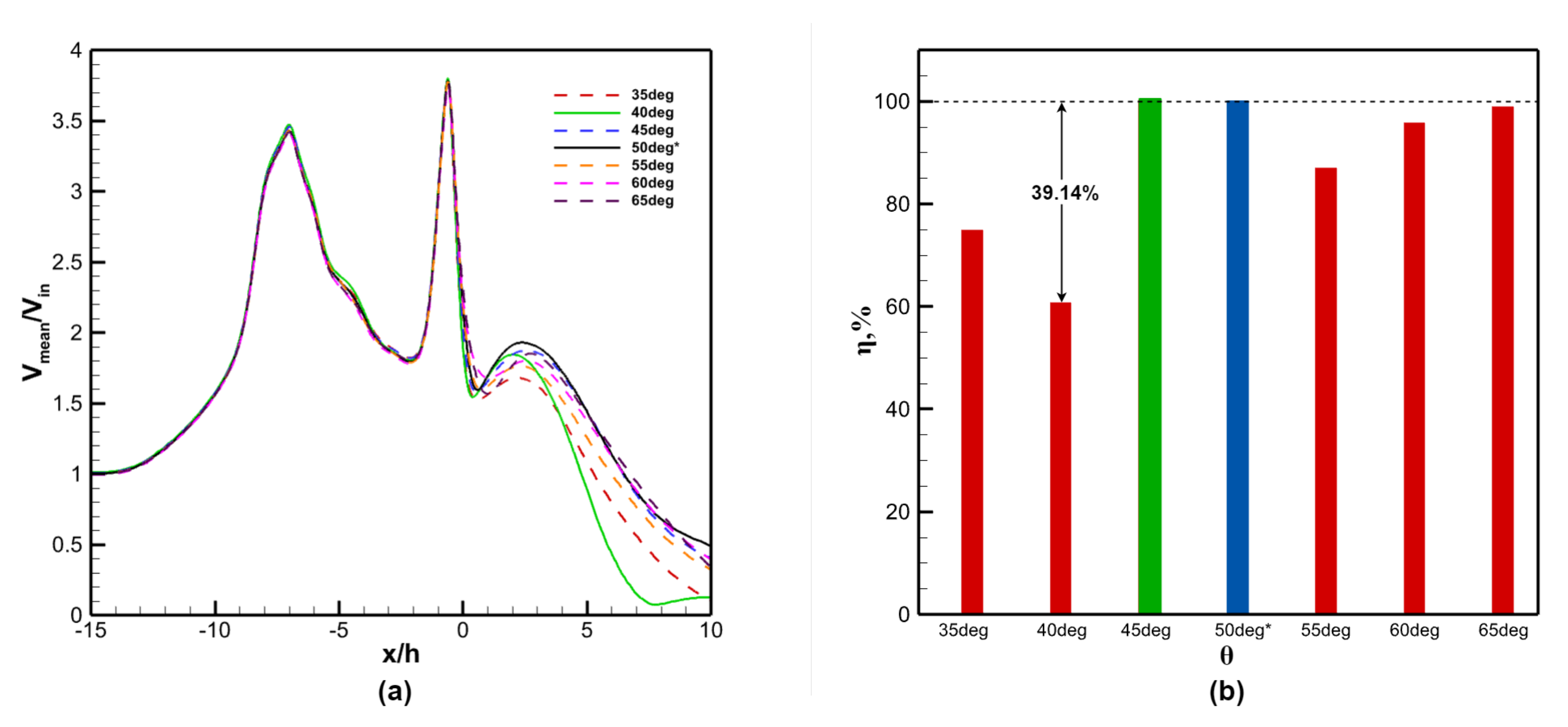
6.2. Effect of Exit Nozzle Angle

To understand the angle effect, the nozzle exit angle was varied from 30${}^{°}$ above and 30${}^{°}$ below the baseline case. Figure 12 shows the time-averaged velocity magnitude along the centerline of the SWJA at different nozzle exit angles. As expected, before the exit nozzle throat, the velocity distribution was almost constant for all the cases. The peak velocity was observed right after the exit nozzle throat, and downstream, the mean velocity dropped for all the cases, except 45${}^{°}$, compared to the baseline case. The velocity ratio at point x/h = 5 showed that only for the 45${}^{°}$ case, we obtained an efficiency at the x/h = 5 location higher than the baseline case (2.34%). The minimum efficiency at that point was 39.15% at 40${}^{°}$. A similar trend can be seen in the pressure field (Figure 9a) as well. The mean pressure distribution along the centerline for the angle cases showed a slight variation in the local pressure. For the smallest angle ($\theta$ = 35${}^{°}$), we obtained the maximum pressure downstream (after x/h = 5). Therefore, the angle cases showed the erratic behavior of the velocity and pressure in the symmetry axis.

FFT analysis exhibited that the oscillation frequency varied from 360 Hz to 340 Hz, within 3% of the frequency of the baseline actuator (Table 3).

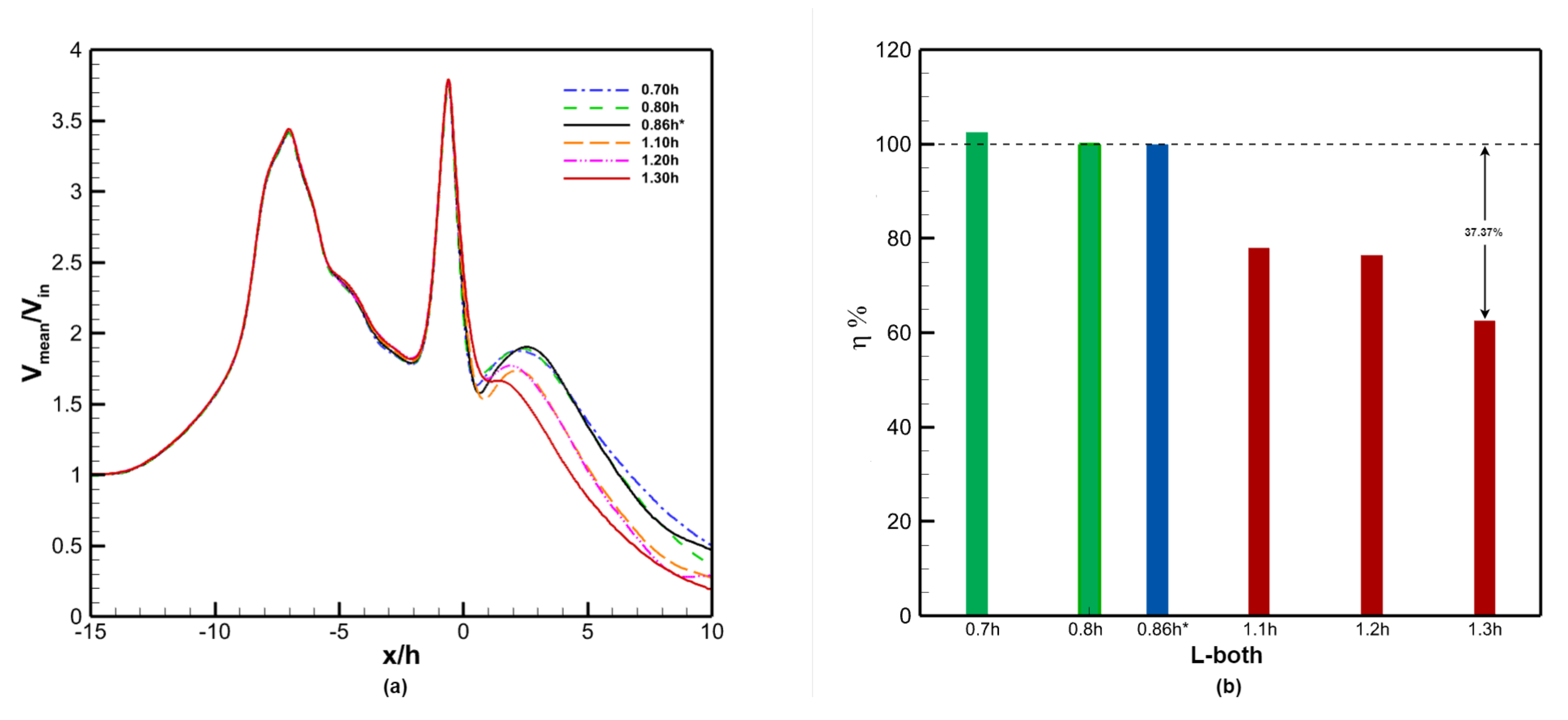
6.3. Effect of Length: Both Nozzle Arms

We studied the L-both case by adjusting the exit nozzle length from 0.70 h to 1.30 h, which increased the nozzle length gradually (both nozzle arms), keeping the baseline case (0.86 h) in between. This resulted in the velocity dropping off 20 m/s after the exit nozzle, which made the shorter nozzle arm length convenient for applications (Figure 13). From the velocity ratio at x/h = 5, it was evident that the velocity decreased gradually starting from 0.70 h to 1.30 h, and the lowest efficiency was 37.37% for the longest arm length (1.30 h) compared to the baseline. The results showed that the increment of the nozzle length caused a slight average pressure rise (Figure 9c). From the FFT analysis (Table 3), it was observed that there was no significant variation in the oscillation frequency (3% with respect to the baseline).

6.4. Effect of Length: Top Nozzle Arm (Asymmetry)

The variation on one side (top) of the exit nozzle length was studied where the other arm of the exit nozzle was kept the same as the baseline for the convenience of the comparison. As the analysis extended from 0.70 h to 1.50 h (the baseline arm length was 0.86 h), this study could reasonably predict the variation for the bottom length cases as well. Compared to the baseline case geometry, the velocity (Figure 14a) for $L_{top}$ decreased with the gradual increment of the arm’s length downstream of the exit nozzle, which indicates asymmetric flow distribution downstream (the velocity profile in given in the Supplementary Materials). When focused at x/h = 5, it was observed that (Figure 14b) the 0.70 h, 0.80 h, and 0.90 h cases performed slightly better compared to the baseline. The velocity ratio decreased up to 52.88% for the longest arm length studied. In the case of pressure (Figure 9d), the longest length had the most gradual increment along the symmetry axis downstream of the diffuser. The oscillation frequency here had a similar magnitude as the baseline (Table 3).

For all the studied cases (Figure 11a), the half-jet width is plotted against the respective parameters (half-exit angle, nozzle length) to compare the jet spreading with the baseline case. From the angle case, a 40${}^{°}$ half-exit angle provided the maximum spreading (0.07252 m higher than the baseline) downstream because of the dual peaks of the mean velocity. In the curvature case, there was a trend showing that the spread gradually decreased from 0.70 h to 1.30 h. For the L-top cases, the jet width increased up to 0.90 h, and then it went down as the nozzle length increased. Finally, L-both showed an upward trend with the nozzle length: higher nozzle length kept the fluid flow attached to the sidewalls, therefore contributing to jet spreading.

7. Conclusions

The present study investigated the effects of exit nozzle geometry on the performance of the sweeping jet actuator (SWJA). First, we investigated the performance of the baseline case and obtained a close agreement with the previous experimental and numerical studies. In the time-accurate analysis, we used a compressible 2D URANS model with the SST k-$\omega$ turbulent closure, which is computationally inexpensive, yet reliable. Then, four different shapes with length adjustments were studied to understand the effect on the oscillation frequency and external flow fields, such as the mean flow velocity and pressure distribution of the SWJA. The FFT analysis result showed that the oscillation frequency was not dependent on the external geometry; it varied with the internal geometry as observed in a previous study [26]. However, for the curvature case, the mean velocity downstream of the exit nozzle was 51.98% higher than the baseline at x/h = 5 due to the Coanda effect at the exit nozzle. Among the studied shapes L-top, L-both, and curvature, each 0.10 h increment in the arm’s length caused a reduction of 9% in the average velocity downstream. Here, the L-top cases created asymmetry in the oscillating jet, and the flow tended to adhere to the longer arm sidewalls. The angle variations showed an erratic behavior for the flow distribution. We observed a negligible mean pressure variation between the cases studied. In conclusion, the SWJA design needs to be modified with the curved exit nozzle configuration for better flow control and uniform jet spreading.

References

1. Cattafesta, L.N., III; Sheplak, M. Actuators for active flow control. Annu. Rev. Fluid Mech. 2011, 43, 247–272. [Google Scholar] [CrossRef] [Green Version]
2. Tomac, M.N.; Gregory, J. Frequency studies and scaling effects of jet interaction in a feedback-free fluidic oscillator. In Proceedings of the 50th AIAA Aerospace Sciences Meeting including the New Horizons Forum and Aerospace Exposition, Tennessee, TN, USA, 9–12 January 2012; p. 1248. [Google Scholar]
3. Tomac, M.N.; Gregory, J. Jet interactions in a feedback-free fluidic oscillator at low flow rate. In Proceedings of the 43rd AIAA Fluid Dynamics Conference, San Jose, CA, USA, 14–17 July 2013; p. 2478. [Google Scholar]
4. Raghu, S. Fluidic oscillators for flow control. Exp. Fluids 2013, 54, 1455. [Google Scholar] [CrossRef]
5. Kara, K.; Kim, D.; Morris, P.J. Flow-separation control using sweeping jet actuator. AIAA J. 2018, 56, 4604–4613. [Google Scholar] [CrossRef]
6. Kara, K. Numerical simulation of a sweeping jet actuator. In Proceedings of the 34th AIAA Applied Aerodynamics Conference, Dallas, DC, USA, 22 June 2015; p. 3261. [Google Scholar]
7. Oz, F.; Kara, K. Jet Oscillation Frequency Characterization of a Sweeping Jet Actuator. Fluids 2020, 5, 72. [Google Scholar] [CrossRef]
8. Kara, K. Numerical study of internal flow structures in a sweeping jet actuator. In Proceedings of the 33rd AIAA Applied Aerodynamics Conference, Atlanta, GA, USA, 16–20 June 2015; p. 2424. [Google Scholar]
9. Koklu, M. Effect of a Coanda extension on the performance of a sweeping-jet actuator. AIAA J. 2016, 54, 1131–1134. [Google Scholar] [CrossRef]
10. Koklu, M. Effects of sweeping jet actuator parameters on flow separation control. AIAA J. 2018, 56, 100–110. [Google Scholar] [CrossRef] [PubMed]
11. Aram, S.; Shan, H. Computational analysis of interaction of a sweeping jet with an attached crossflow. AIAA J. 2019, 57, 682–695. [Google Scholar] [CrossRef]
12. Bohan, B.T.; Polanka, M.D. The Effect of Scale and Working Fluid on Sweeping Jet Frequency and Oscillation Angle. J. Fluids Eng. 2020, 142, 061206. [Google Scholar] [CrossRef]
13. Hirsch, D.; Gharib, M. Schlieren visualization and analysis of sweeping jet actuator dynamics. AIAA J. 2018, 56, 2947–2960. [Google Scholar] [CrossRef]
14. Ott, C.; Gallas, Q.; Delva, J.; Lippert, M.; Keirsbulck, L. High frequency characterization of a sweeping jet actuator. Sens. Actuators A Phys. 2019, 291, 39–47. [Google Scholar] [CrossRef] [Green Version]
15. Jeong, H.S.; Kim, K.Y. Shape optimization of a feedback-channel fluidic oscillator. Eng. Appl. Comput. Fluid Mech. 2018, 12, 169–181. [Google Scholar] [CrossRef] [Green Version]
16. Lin, J.C.; Whalen, E.A.; Andino, M.Y.; Graff, E.C.; Lacy, D.S.; Washburn, A.E.; Gharib, M.; Wygnanski, I.J. Full-Scale Testing of Active Flow Control Applied to a Vertical Tail. J. Aircr. 2019, 56, 1376–1386. [Google Scholar] [CrossRef]
17. Park, T.; Kara, K.; Kim, D. Flow structure and heat transfer of a sweeping jet impinging on a flat wall. Int. J. Heat Mass Transf. 2018, 124, 920–928. [Google Scholar] [CrossRef]
18. Pack Melton, L.G.; Lin, J.C.; Hannon, J.; Koklu, M.; Andino, M.; Paschal, K.B. Sweeping Jet Flow Control on the Simplified High-Lift Version of the Common Research Model. In Proceedings of the AIAA Aviation 2019 Forum, Dallas, TX, USA, 17–21 June 2019; p. 3726. [Google Scholar]
19. Ostermann, F.; Woszidlo, R.; Nayeri, C.; Paschereit, C. Interaction Between a Crossflow and a Spatially Oscillating Jet at Various Angles. AIAA J. 2020, 58, 2450–2461. [Google Scholar] [CrossRef]
20. Park, S.; Ko, H.; Kang, M.; Lee, Y. Characteristics of a Supersonic Fluidic Oscillator Using Design of Experiment. AIAA J. 2020, 58, 2784–2789. [Google Scholar] [CrossRef]
21. Wilcox, D.C. Turbulence Modeling for CFD; DCW Industries: La Canada, CA, USA, 1998; Volume 2. [Google Scholar]
22. Menter, F.R. Two-equation eddy-viscosity turbulence models for engineering applications. AIAA J. 1994, 32, 1598–1605. [Google Scholar] [CrossRef] [Green Version]
23. Ansys®Fluent, Release 2020 R1, User Guide; ANSYS, Inc.: Canonsburg, PA, USA, 2021.
24. Slupski, B.J.; Tajik, A.R.; Parezanović, V.B.; Kara, K. On the impact of geometry scaling and mass flow rate on the frequency of a sweeping jet actuator. FME Trans. 2019, 47, 599–607. [Google Scholar] [CrossRef] [Green Version]
25. Vatsa, V.; Koklu, M.; Wygnanski, I. Numerical simulation of fluidic actuators for flow control applications. In Proceedings of the 6th AIAA Flow Control Conference, New Orleans, LA, USA, 25–28 June 2012; p. 3239. [Google Scholar]
26. Tajik, A.R.; Kara, K.; Parezanović, V. Sensitivity of a fluidic oscillator to modifications of feedback channel and mixing chamber geometry. Exp. Fluids 2021, 62, 250. [Google Scholar] [CrossRef]
Figure 1. Computational domain of the SWJA and the flow field (baseline) showing the inlet and outlet.
Fluids 07 00069 g001
Figure 2. Schematic diagram of the sweeping jet actuator including the tested geometric parameters of the exit nozzle, (a) variation in the angle, where θ = half exit nozzle angle, (b) top arm length variation, L-top, (c) both arm lengths’ variation, L-both, and (d) curvature variation, where L = nozzle length, the horizontal distance starting from the throat up to the nozzle end.
Fluids 07 00069 g002
Figure 3. (Left) SWJA geometry showing the position of different sampling points, uf, lf, and x6y0, exit nozzle height, h, exit nozzle length, l, with global coordinates (blue arrow), and Sphere of Influence 1 (red circle) used for focused meshing. (Right) Close view of the mesh near the exit nozzle region.
Fluids 07 00069 g003
Figure 4. (a) Time history at three different locations (P-uf), (P-lf), and (P-x6y0) showing the pressure amplitude for N-60 (only the clipped portion of the sample) and corresponding FFT analysis (b) at those sampling locations where peaks indicate the oscillation frequency, respectively.
Fluids 07 00069 g004
Figure 5. Oscillation frequency obtained from FFT analysis for 0.1s at different sampling points based on the velocity magnitude (v) and static pressure (p): downstream, x6y0 (6 mm, 0 mm), upper feedback channel, uf (−25.4 mm, 19 mm), and lower feedback channel, lf (−25.4 mm, −19 mm), for different mesh distributions.
Fluids 07 00069 g005
Figure 6. Local error analysis of the mean pressure along the centerline based on the finest (N-80) mesh. The mean pressure is normalized by the inlet mean pressure P i n = 128,961.46 Pa.
Fluids 07 00069 g006
Figure 7. Local error analysis of the mean velocity along the centerline based on the finest (N-80) mesh. The mean velocity is normalized by the inlet mean velocity V i n = 44.83 m/s.
Fluids 07 00069 g007
Figure 8. (a) Mean velocity along the centerline normalized by the inlet velocity, V i n , B a s e l i n e ; (b) velocity ratio, η , at point x/h = 5 for the curvature case.
Fluids 07 00069 g008
Figure 9. Mean pressure along the centerline nondimensionalized with the inlet pressure, P i n , B a s e l i n e for (a) Angle, (b) Curvature, (c) L-both and (d) L-top.
Fluids 07 00069 g009
Figure 10. Instantaneous total pressure along the centerline normalized with the total inlet pressure, P t o t a l , B a s e l i n e = 131,829.6584 Pa for curvature cases.
Fluids 07 00069 g010
Figure 11. At x/h = 5, (a) half-jet width for curvature, L-top and L-both cases (in terms of nozzle length, x/h) and angle case (in terms of the half-exit angle, θ ). (b) Velocity profile for the curvature case.
Fluids 07 00069 g011
Figure 12. (a) Mean velocity along the centerline normalized by the inlet velocity, V i n , B a s e l i n e ; (b) velocity ratio, η , at point x/h = 5 for the angular case.
Fluids 07 00069 g012
Figure 13. (a) Mean velocity along the centerline normalized by the inlet velocity, V i n , B a s e l i n e ; (b) velocity ratio, η , at point x/h = 5 for the L-both case.
Fluids 07 00069 g013
Figure 14. (a) Mean velocity along the centerline normalized by the inlet velocity, V i n , B a s e l i n e ; (b) velocity ratio, η at point x/h = 5 for the L-top case.
Fluids 07 00069 g014