Article

Analysis of a Stator-Rotor-Stator Spinning Disk Reactor in Single-Phase and Two-Phase Boiling Conditions Using a Thermo-Fluid Flow Network and CFD

by
Lorenzo Mazzei
1,*,
Francesco Maria Marin
2,3,
Cosimo Bianchini
1,
Riccardo Da Soghe
1,
Cristina Bertani
2,
Dario Pastrone
2,
Maddalena Angelucci
3,
Giuseppe Caggiano
3 and
Michiel de Beer
4,†
1
Ergon Research s.r.l., Via Giuseppe Campani, 50, 50127 Florence, Italy
2
Politecnico di Torino, C.so Duca degli Abruzzi 24, 10129 Torino, Italy
3
Avio S.p.A., Via I Maggio, 56, 10040 Torino, Italy
4
Laboratory of Chemical Reactor Engineering, Department of Chemical Engineering and Chemistry, Eindhoven University of Technology, 5600 MB Eindhoven, The Netherlands
*
Author to whom correspondence should be addressed.
Current Affiliation: Nobian Industrial Chemicals B.V., 6824 BM Arnhem, The Netherlands.
Fluids 2022, 7(2), 42; https://doi.org/10.3390/fluids7020042
Submission received: 1 December 2021 / Revised: 11 January 2022 / Accepted: 13 January 2022 / Published: 18 January 2022
(This article belongs to the Special Issue Multiphase Flow in Pipes with and without Porous Media)

Abstract

:
Cryogenic liquid propellants are used in liquid rocket engines to obtain high specific impulse. The flow rates are controlled by turbopumps that deliver liquid propellant to the engine at high pressure levels. Due to the very low saturation temperature of the cryogenic propellant, in the first phases of the transient operation, in which the engine is at ambient temperature, its surfaces are subject to boiling conditions. The effect of boiling on the heat transfer between the solid and the fluid needs to be well characterized in order to correctly predict the cryopump metal temperature temporal evolution and the necessary amount of propellant. With the aim of benchmarking numerical tools against experimental data, a representative test case was chosen. This consists of a stator-rotor-stator spinning disc reactor studied under single-phase and two-phase heat transfer conditions. The numerical approaches used are represented by a 1D network solver, where the pressure drop and heat transfer are calculated by correlations, and Computational Fluid Dynamics (CFD) simulations, carried out with ANSYS Fluent. Both the numerical tools returned a reasonable agreement in single-phase conditions, also thanks to the use of adequate correlations in the flow network solver and typical conditions for the CFD simulations. Two-phase conditions on the contrary are more challenging, with underpredictions up to 20% and 80%, respectively. The issues are ascribable to the use of correlations that are inadequate to capture the two-phase phenomena occurring in the srs reactor and numerical limitations in the actual implementation of the boiling model in the CFD solver.

1. Introduction

Two-phase heat transfer is present in many engineering applications. It is particularly attractive for thermal management applications due to its inherent capability to deliver very high heat transfer rates. Its nature makes it very challenging to model and, for historical reasons, investigations have focused mainly on nuclear-relevant conditions, that is, with a particular emphasis on pressurized water and subcooled/saturated nucleate boiling. Despite that, two-phase heat transfer can also occur in very different applications, such as the chilldown process taking place at the start-up of rocket engines. During this phase, the feed line and the turbopump is brought from ambient temperature to the nominal cryogenic condition required to avoid vapor phase propellant entering the turbopump and the thrust chamber during engine ignition. The coolant used during the procedure is the propellant itself, which is allowed to flow inside the feed lines and the turbopump until the correct wall temperature is reached. During the chilldown of the turbopump, a variety of flow conditions are encountered, including two-phase flow regimes, which must be adequately described. The procedure can last minutes and an accurate prediction may reduce the propellant mass dedicated to the chilldown phase. Flow networks and CFD simulations may serve the purpose, estimating the thermal boundary conditions for a transient thermo-mechanical simulation of the system [1].
Flow network solvers are the most appropriate tools to preliminary design and analyse components and systems of the two-phase heat transfer phenomena. This approach relies on 1D modelling, therefore complex 3D problems must be simplified and typically represented by a series of interconnected elements linked by nodes, composing the equivalent flow network. An example of this is the analysis conducted by Li et al. [2], where the chilldown of a feed line with a centrifugal turbopump at the end was investigated. In their study, Li et al. [2] neglected the internal geometry of the turbopump, modelling it as a pipe with an equivalent mass and diameter. However, Van Hooser at al. [3] showed that it is possible to correctly simulate the fluid flows inside an operative turbopump by increasing the complexity of the fluid network. Unfortunately, the network used did not model wall-fluid heat transfer and it could not be used to simulate a chilldown of the pump, but it showed that fluid networks could indeed be used to simulate geometries as complex as those of a turbopump. It is necessary to point out that fluid network solvers make use of bulk properties averaged over a cross-sectional area normal to the mean flow and need sets of correlations based on experimental data for well-established flows. Their prediction accuracy is heavily influenced by the accuracy of the chosen correlations. So, reviews of the performances of the different correlations for various fluids and geometries, such as those published by Kim and Mudawar [4] (room temperature fluids) and Hartwig et al. [5,6] (cryogens), are needed to choose the most suitable correlations. Despite such limitations, fluid network solvers offer robustness, fast calculations and good accuracy, if used in their validity range.
Computational Fluid Dynamics (CFD) can be exploited to investigate boiling problems, typically using different mechanistic models depending on the regime of interest. Three dimensional (3D) CFD in fact allow us to account for realistic geometrical features, variable boundary conditions in space and time as well as complex flow fields. This represents a considerable advantage compared to empirical approaches based on 1D flow networks or simplified scenarios such as straight channels, pool or thin film boiling. Despite that, the accuracy of CFD in predicting boiling flows strongly relies on the implemented boiling models, which are usually developed for a specific regime. The RPI wall boiling model, for example, developed by Kurul and Podowski [7] at the Rensselaer Polytechnic Institute, is acknowledged as a good choice for CFD simulations in an Eulerian multiphase framework. The model has been widely used in the nuclear industry and, in general, for high-pressure, steam-water systems. However, some issues were observed with this approach at lower operating pressure levels [8] and outside of the nucleate boiling regime. Software like the ANSYS Fluent feature has additional models, typically modifications of the RPI model, with different formulations capable of modelling the heat transfer and multiphase conditions at critical heat flux and post dry-out regimes. With the aim of addressing the poor performance in low-pressure conditions, Das and Punekar [9] developed a new wall boiling model for the mixture multiphase framework. The Semi Mechanistic Boiling (SMB) model is meant to provide a robust, computationally friendly and reasonably accurate approach also for complex-shaped coolant passages. The boiling modelling available in Fluent was benchmarked by Bianchini et al. [10], assessing the predicting capability in numerous test cases: namely nucleate boiling of sub-cooled water in an upward heated cylindrical pipe (Bartolomej et al. [11]), boiling water in a rectangular-sectioned duct (Pierre and Bankoff [12]), nucleate boiling with the R-113 refrigerant as an alternative to water (Roy et al. [13]) and critical heat flux and post dry-out regimes of water in vertical pipes (Becker et al. [14]). Despite that, a proper validation of rotating conditions is still lacking and valuable in the perspective of an application in the turbomachinery context.
In the following article, the stator-rotor-stator spinning disk reactor (srs-SDR) studied by de Beer et al. [15,16] is analysed using a thermo-fluid network solver previously developed to analyse the chilldown process inside the metallic piping feeding the cryopump. In addition, CFD simulations performed with ANSYS Fluent, previously validated on literature test cases [10], were considered to carry out the validation of such modelling. The srs-SDR was chosen as a test case to verify the tool predictions for a more complex geometry and more relevant fluid-dynamic conditions. The test case offers experimental data on different fluids (water and dichloromethane) and different heat transfer scenarios (single-phase and two-phase), as well as both stationary and rotating conditions. In addition, it considers a low-pressure level and mini annular channels between circular disks. The test case was initially analysed in single-phase conditions and subsequently the two-phase heat transfer was considered. The benchmark of the tools will be valuable for their subsequent exploitation for design and analysis purposes.

2. Single-Phase Flow

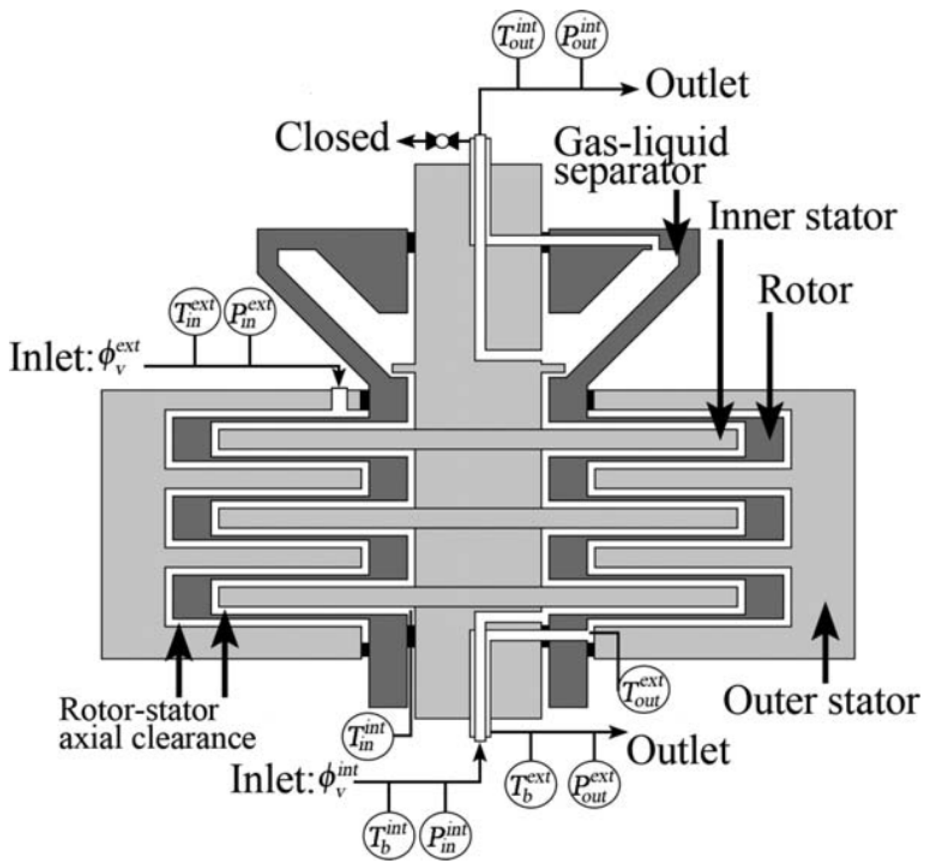
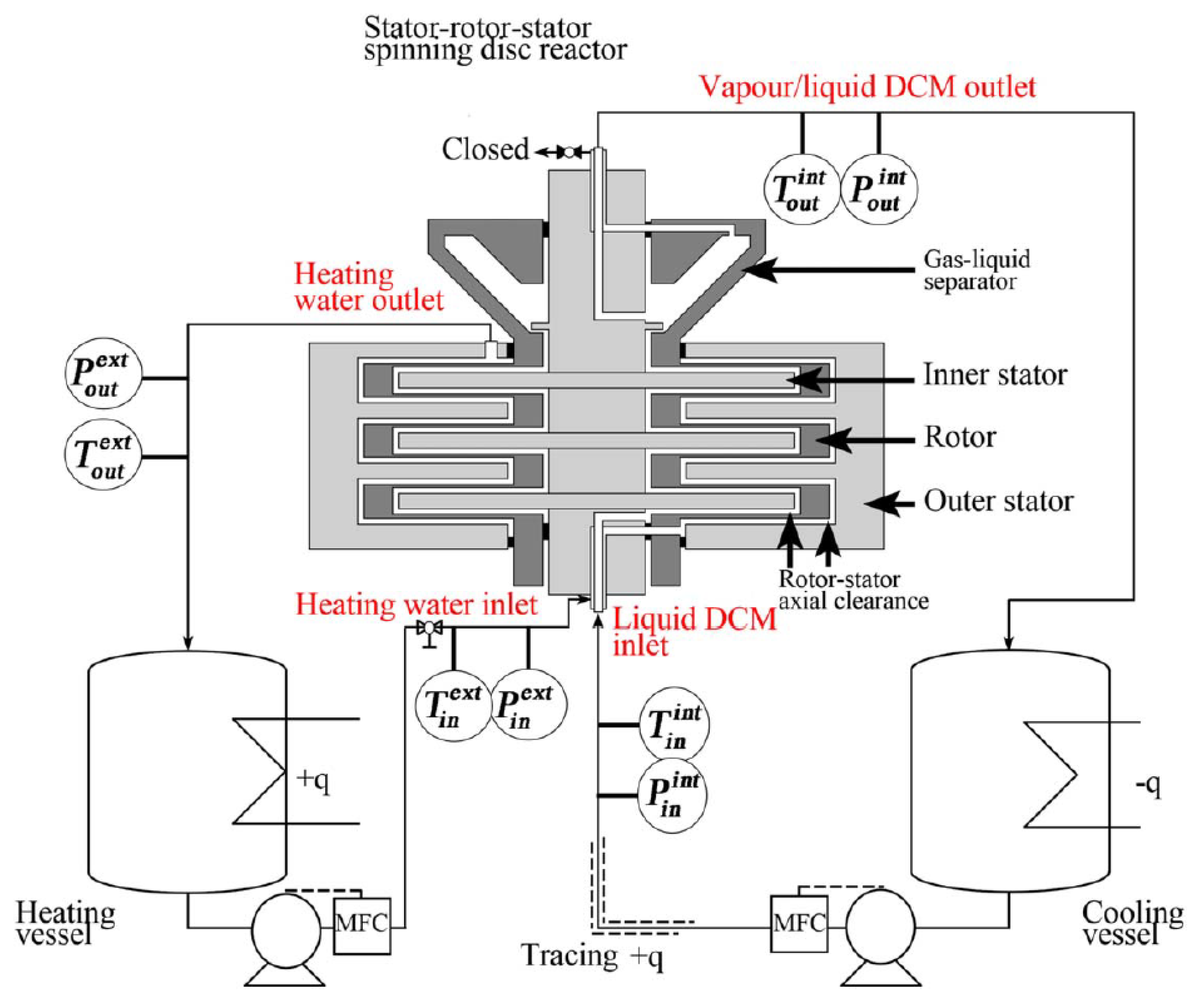
2.1. Test Case Description

A sketch of the geometry tested by de Beer et al. [15] during the single-phase campaign is depicted in Figure 1.
The srs-SDR is composed of three different stages, identical to each other. Each stage of the reactor consists of a disc connected to a central shaft (inner stator), which is surrounded by movable housing (rotor). The rotor is spun by an electrical motor, with a rotational speed of up to 209 rad/s. Between the inner stator and the rotor there is a 2 mm gap where a fluid can flow. The rotor itself is surrounded by its own housing (outer stator) with a 2 mm gap between the outer stator and the rotor, forming a second annular passage for fluid flow. The reactor outer walls are thermally insulated using an HT/Armaflex® insulator, to avoid heat losses. The two circuits inside the reactor are physically isolated from each other. However, the flows in the two cavities can exchange heat through the rotor, mainly in the area where the rotor is thinner (1 mm), at radii between 28 mm and 60.5 mm. For radii outside the previous range, the rotor is 10.5 mm thick. The reactor is made of 316 L stainless steel and a thermal conductivity of 16 W/(m K) was assumed during the simulations. Table 1 summarises the dimensions of the various components:
Coriolis flow controllers are also installed on both feed lines to regulate the flows entering the reactor. A gas–liquid separator is mounted on the rotor at the top of the reactor, in order to separate the two phases at the outlet of the internal cavity (which was used only for the two-phase experimental runs).
The placement of the different sensors is shown in Figure 1. The temperature at the inlet of the interior cavity is not directly measured and it was determined by de Beer et al. [15] by imposing an energy balance over the feed line at the bottom of the reactor. Gauge pressures were also measured at the inlet and outlet of each cavity and were later corrected, accounting for the hydrostatic pressure.
Concerning the uncertainty associated to measurements, an error of T ± 0.06 K for temperature and P ± 400 Pa for pressure was reported. Concerning the flow rate measurements, the error was estimated to be equal to ϕ L ± 0.08 × 10 6 m 3 /s for the volumetric flow rate of water on both sides of the srs SDR. At last, ω ± 0.05 rad/s for the rotational velocity.
For the single-phase experimental runs, the rotor speed was varied between 0 and 160 rad/s, at two different flow rates in the two cavities (15 mL/s and 20 mL/s). The influence of mass flow and rotor speed on the heat transfer coefficients has been studied during the experiment.
The srs reactor performance was evaluated with distilled water flowing in both internal and external cavities. During these runs, the reactor operated in counterflow mode. Heated water was injected in the outer circuit at a temperature between 40 and 42 °C, while distilled water entered in the internal cavity at a lower temperature, between 23 and 25 °C. Measured output data consisted of pressure (to estimate the pressure drop), outlet temperature (to estimate the thermal power exchanged) and torque at the shaft. Experimental data were gathered for variable rotor speeds and two different values of internal mass flow (15 mL/s and 20 mL/s), while the external mass flow was kept constant.
For all the details concerning the test case and the measurement techniques employed, the interested reader can refer to de Beer et al. [15].
The simulations performed in this study aimed to reproduce the observed heat exchange effectiveness, calculated as:
η = Q T Q m a x = ρ L c p , L ϕ L e x t ( T i n e x t T o u t e x t ) ρ L c p , L ϕ L e x t ( T i n e x t T i n i n t ) = T i n e x t T o u t e x t T i n e x t T i n i n t .
The predicted overall heat transfer coefficients have also been compared to the ones presented by de Beer et al. [15] in their study.

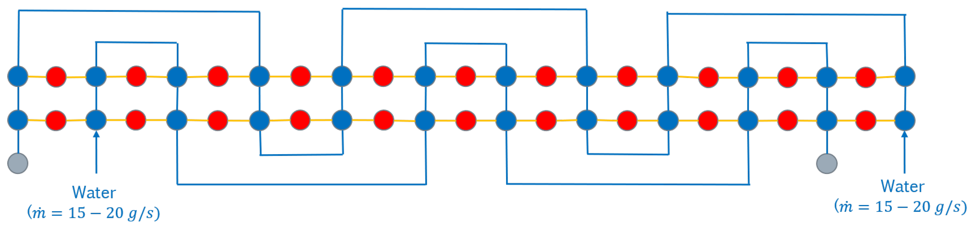
2.2. 1D Network—Test Case Modelling

Two different networks were used to model the srs reactor. The first one (see Figure 2) modelled only the two cavities and the rotor. Heat fluxes through the stators were so neglected. Eight fluid nodes were used to model each stage of the srs reactor (four for each circuits). Two additional nodes were used to impose boundary conditions (outlet pressure of each circuit). The other boundary conditions were imposed using a fixed mass flow at the inlet of each channel with a given temperature (40 °C for the outer channel and 25 °C for the inner one).
The rotor is modelled using twelve nodes, four for each stage. Every solid node is connected to two different fluid nodes of the two cavities and the correlations presented in the next section were used to model the heat transfer between these nodes.
A second set of simulations was performed using a more detailed network. This second network included additional solid nodes that modelled the two stators. The fluid nodes of one circuit were so able to exchange heat not only with fluid nodes of the other circuit, but also with fluid nodes of the same circuit. Only Equation (4) has been used for the stators, as de Beer et al. [15] highlighted that the transition to turbulent flow for the stators occurred at much lower Reynolds numbers than for the rotor. A schematic of the updated network is reported below in Figure 3:

2.3. 1D Network—Heat Transfer and Pressure Drop Modelling

The MATLAB code used to simulate the srs reactor required dedicated correlations in order to model the heat transfer between fluid and wall. The correlations developed by de Beer et al. in the original article [15] were chosen and inserted into the simulation tool. The correlations were proposed for each one of the three different flow regimes occurring on the rotor wall (i.e., laminar, transition and turbulent):
N u r l a m = 1.4 R e ω 0.5 R e ω < 1.1 × 10 5
N u r t r a n s = 3.5 × 10 9 R e ω 2.14 + 267 1.1 × 10 5 < R e ω < 2.3 × 10 5
N u r t u r b = 0.073 R e ω 0.8 R e ω > 2.3 × 10 5 ,
with R e ω = ω r 2 ν f and N u r = h f r r o t e x t k f . This set of correlations predicts a heat transfer coefficient equal to zero when ω = 0 . So, a lower limit to the heat transfer coefficient was imposed, assuming N u D H equal to 5.385 (recommended value for laminar convection in a flat channel with one adiabatic walls [17]). It was also necessary to take into account the power dissipated by the rotor into the fluid. Another correlation developed by de Beer et al. [15] was used:
P d p = 6 × ( 5.73 × 10 12 G r , e x t 0.14 ( R e ω e x t ) 2.12 ) ,
where G r , e x t = s r e x t . The calculated power has been divided between the different fluid nodes of the network, constituting an additional term in the fluid enthalpy conservation equation.
Pressure drop data available in the reference article did include losses caused by the reactor feed lines and it was not possible to establish precisely the pressure drop across the reactor. The reactor pressure drop was calculated assuming a circular pipe with the same length of the reactor and an equivalent diameter obtained from the available data. The influence of rotor speed on pressure losses was not considered.

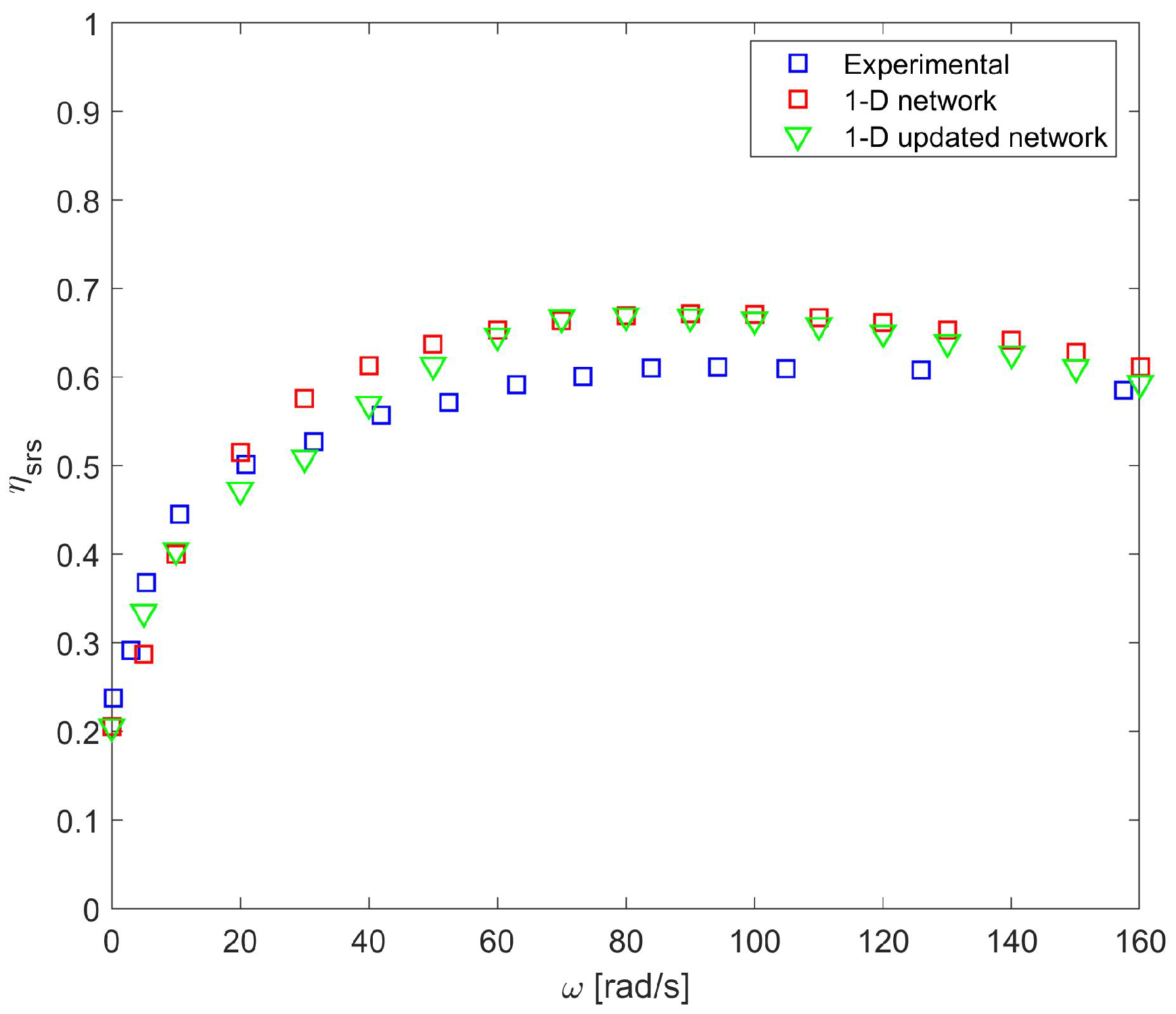
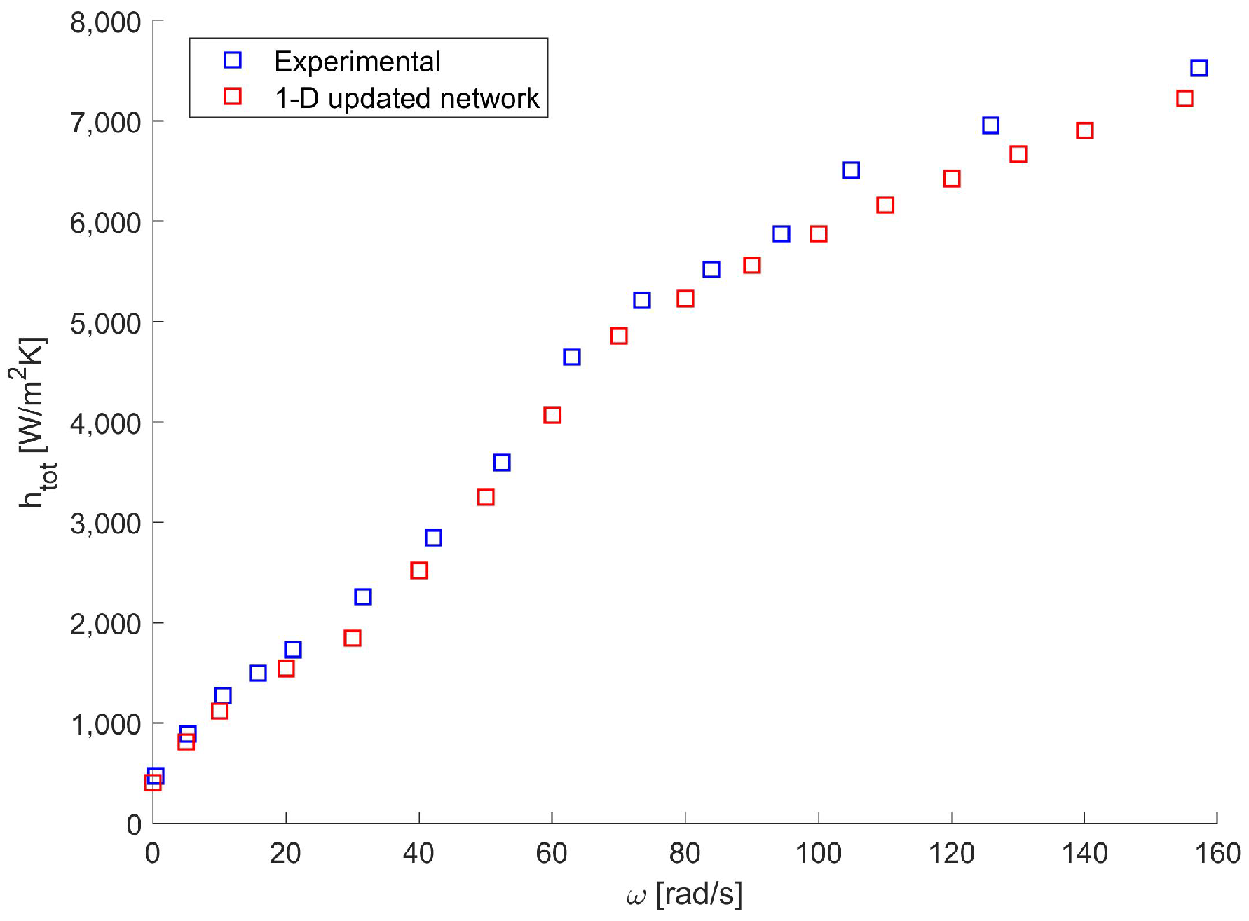
2.4. 1D Network—Results

The results of the simulations performed with the two different networks were compared with the experimental data of de Beer et al. [15] to establish the accuracy of the simulation tool. The comparison is reported in Figure 4 and Figure 5 for the two different mass flows used during the experiment.
It is possible to see that the heat exchange effectiveness predicted by the simulations and the one measured experimentally show similar trends when reported as a function of the rotor’s rotational speed. There is a sharp increase in heat exchange effectiveness between 0 and 40 rad/s. However, the gain in terms of heat exchange effectiveness is gradually reduced for higher values of angular velocity, and it even starts to decrease when ω is higher than 80 rad/s. This is due to the increase in the power dissipated by the rotor, as reported by de Beer et al. [15]. This hampers the cooling of the fluid in the external circuit. At the same time, the fluid wall heat transfer coefficient is so high that the rotor conductive thermal resistance is no longer negligible, with a consequent reduction of the influence of ω on the heat fluxes between the two circuits.
The differences between the results using the two different networks are most evident for low values of ω , where the simulations using the updated network shows better agreement with the experimental data and predicts lower values of heat exchange effectiveness. The inclusion of the stators inside the network leads to a lower mean temperature differential between the circuits, so reducing the heat exchanged. The difference between the two networks becomes negligible for higher values of ω for two reasons:
  • Conduction becomes the limiting factor for the heat fluxes through the stators. This phenomenon affects also the rotor, but at higher rotational speeds, due to different thicknesses of the two components (4 mm for the stators and only 1 mm for the rotor);
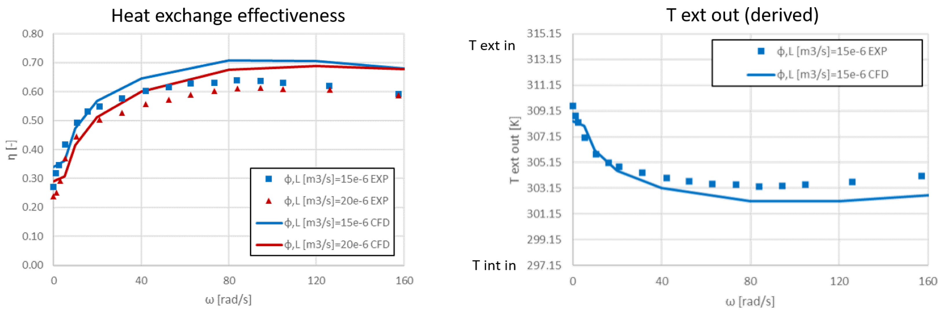
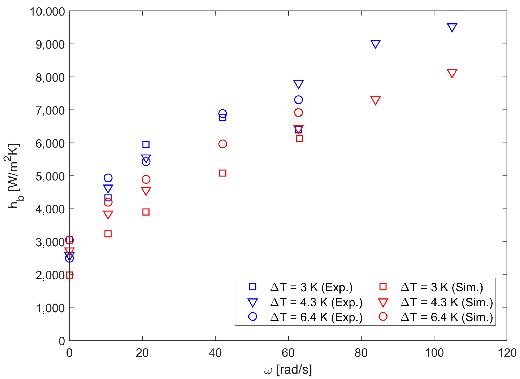
  • Flow regime transition occurs on the rotor for values of ω between 40 rad/s and 60 rad/s. The simulation tool switches between the three different correlations available, with an increase in the convective heat transfer coefficient. This does not occur for the stators, where only Equation (4) is used.
This second effect is visible in Figure 6 when comparing the experimental and calculated mean overall heat transfer coefficient, which is defined as:
h t o t = 1 h e x t , m + d r k r + 1 h b , m 1 .
The simulation tool appears to predict slightly lower heat transfer coefficients, but it shows a very similar trend as a function of ω .
Overall, the simulations showed a satisfactory accuracy when compared against single-phase experimental data, especially when using the updated network and for lower rotational velocities. The error in the prediction of the heat exchange effectiveness is always lower than 10%.

2.5. CFD—Test Case Modelling
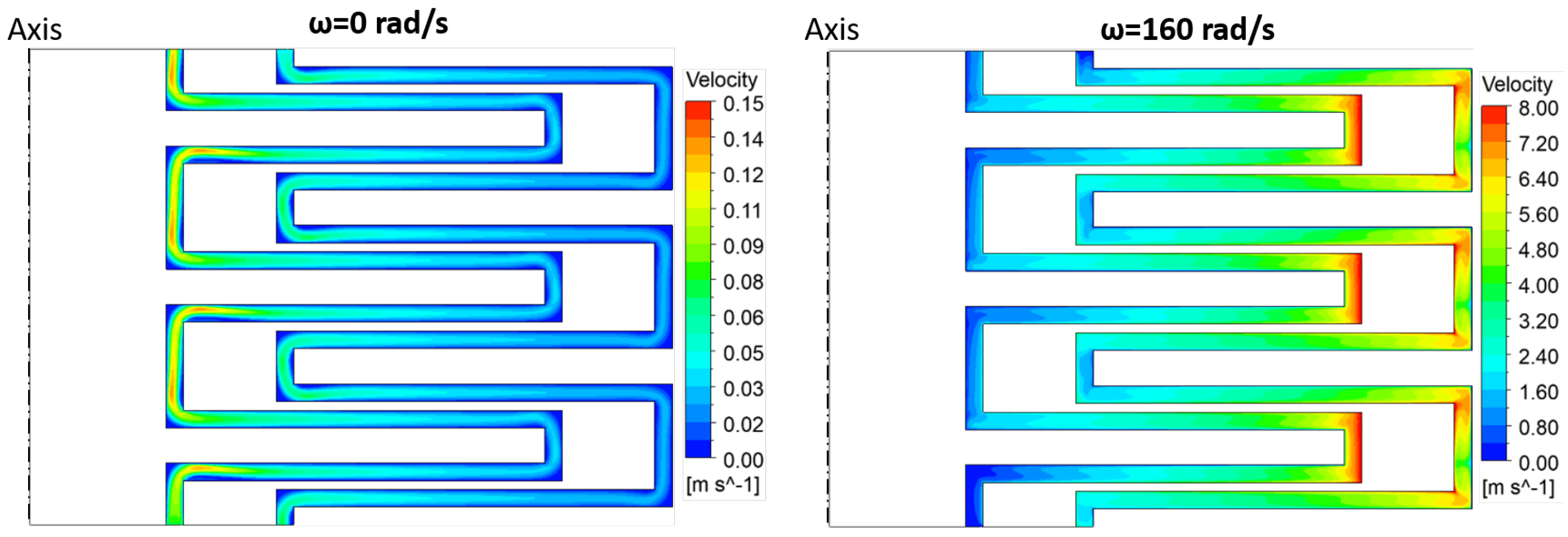
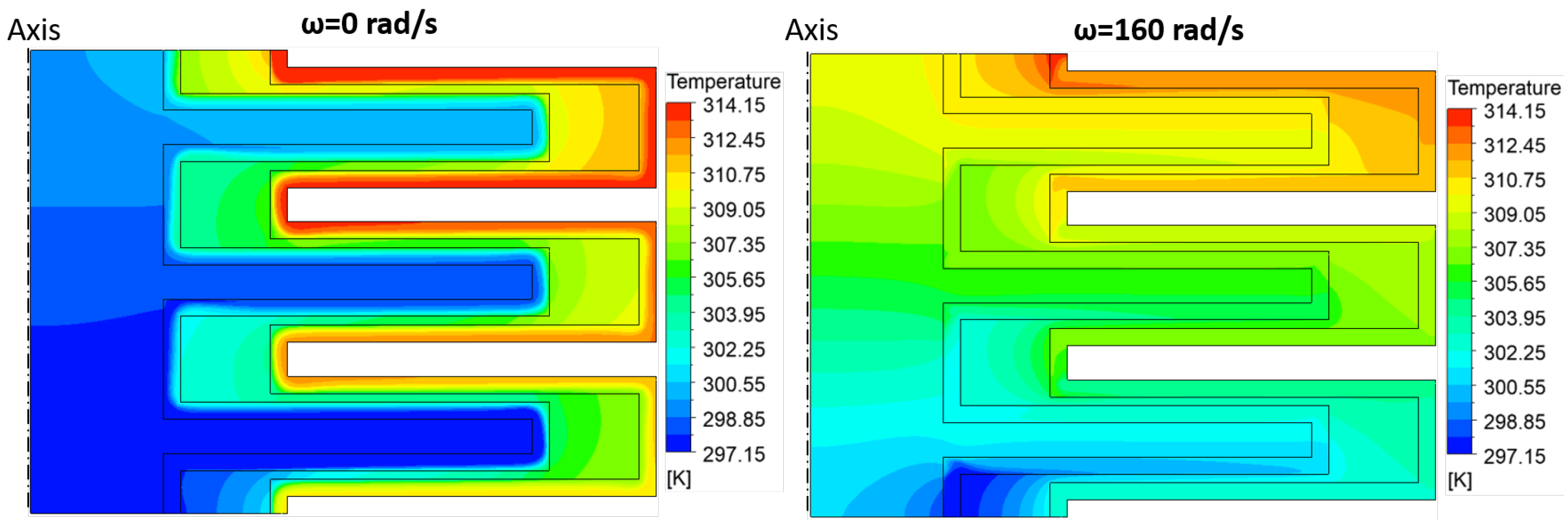
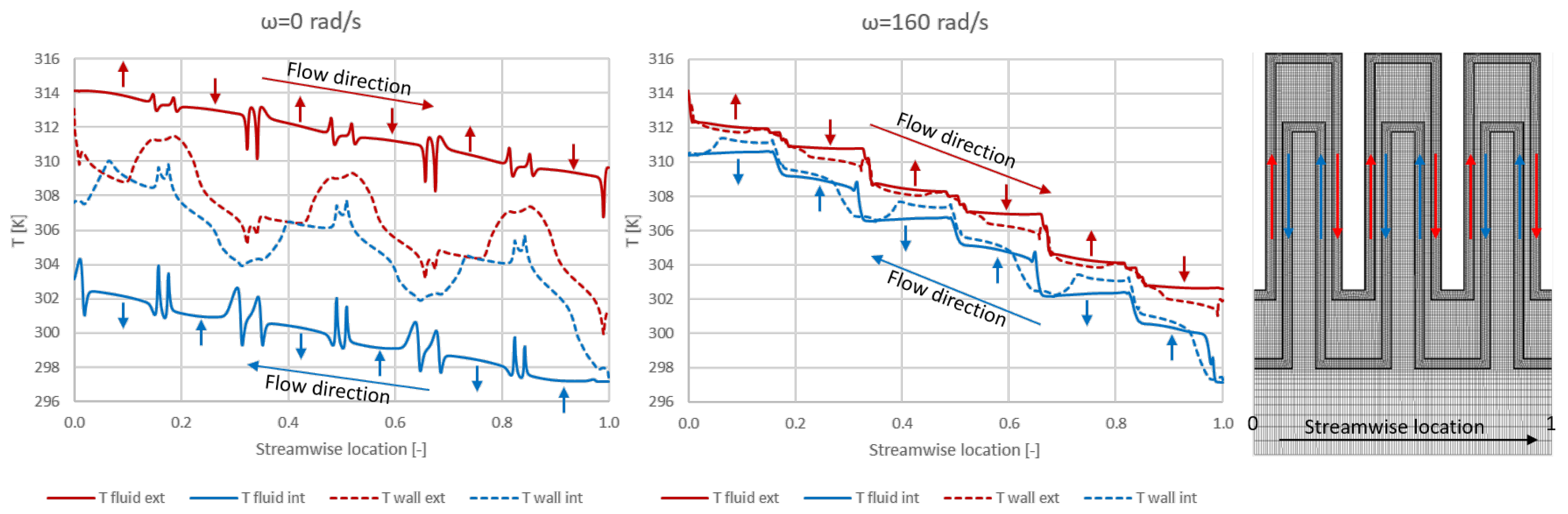
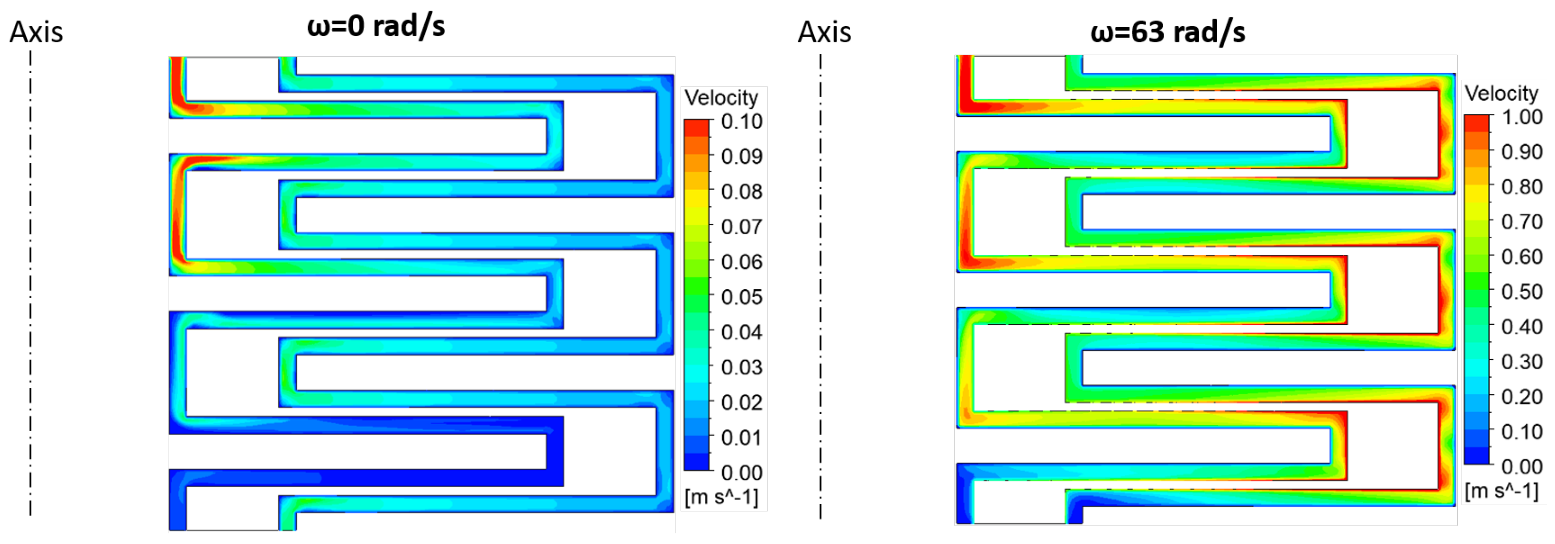
The results reported in this paper were obtained with the commercial software ANSYS Fluent 2019R3. The test case was modelled as a 2D problem thanks to the axisymmetric nature of the geometry and the steady-state assumption. The computational grid was generated in ICEM-CFD and is reported in Figure 7. As it is possible to notice, the single-phase cases consist of a Conjugate Heat Transfer (CHT) including the internal stator and the rotor. “Cold” water flows from bottom to top, while “hot” water enters the upper part in a counter-flow arrangement. The fluid–solid interfaces between such domains are coupled, meaning that the same temperature is achieved on the two sides and the heat is conserved through the interface ( T f = T s , q f = q s ). The other sides of the solid domains, as well as the surface of the “hot” water in contact with the external stator, are considered adiabatic.
All the walls are considered smooth (due to the low roughness of the test article) and are characterized by a no slip condition. Inlets were characterized by means of inlet velocity (chosen to match the mass flow rate measured in experimental tests) and total temperature. In the absence of more detailed information, the direction of the flow is imposed as normal to the boundary. At the outlets a static pressure level is prescribed.
The gravitational effects were included in the simulation, despite the negligible effects if compared to two-phase conditions. Turbulence effects were modelled by means of the k ω SST turbulence model with a wall integration treatment, similarly to what had been done previously in Bianchini et al. [10], where the CFD model was validated on several literature test cases. Constant properties were assumed for water due to the limited temperature range investigated in the tests.

2.6. CFD—Results

The results of the CFD simulations for the single-phase conditions are reported in this section. The first results reported consist of the velocity fields, under stationary and rotating conditions (see Figure 8). As it is possible to observe, on equal mass flow rate the rotation has a strong impact on the flow conditions. As highlighted also by de Beer et al. [18], the rotational speed of 160 rad/s is sufficient to bring the flow from laminar to fully turbulent conditions in terms of rotational Reynolds number. This is also confirmed qualitatively by the velocity contours. Under laminar conditions, the flow is prone to separation downstream of curves and is characterized by a reduction in velocity when moving to high radii (due to the increase in passage section). On the contrary, when dealing with rotational conditions, the flow exhibits a stronger uniformity due to strong wall shear, which also indicates stronger gradients and ultimately higher transfer levels. It is also worth pointing out that the velocity gradually increases, moving to higher radii due to the increase in tangential velocity.
Additional rotational effects are visible, observing the static pressure contours reported in Figure 9. It is possible to notice how, under stationary conditions, the pressure variations are small, with the pressure gradually and monotonically reducing, moving from the inlets to the outlets. As far as the rotating conditions are concerned, the overall reduction in pressure is preserved, while the pumping effect of rotating walls makes the trend non-monotonic.
The impact of rotation is even more evident when looking at the temperature distribution within the reactor (in both fluid and solid). As visible in Figure 10, the stationary condition returns high temperature differences between “hot” and “cold” water, as the laminar flow represents the bottleneck in the heat exchange process due to the limited mass/thermal transport. Very different results are achieved under rotating conditions, with a significantly smoother temperature distribution. This clearly confirms the increase in heat transfer provided by the fluid for fully turbulent conditions, which results in a higher “effective” thermal conductivity.
To obtain a more quantitative insight into the results, temperature profiles were extracted and plotted in Figure 11, considering the center of the fluid channels (continuous lines) and the fluid–solid interface (dashed lines). The data were arranged to evaluate the streamwise location (the curvilinear abscissa) in non-dimensional terms, 0 being the entrance of the “hot” water and 1 the exit. By doing so, it is possible to appreciate the impact of rotation. Under stationary conditions, the average local temperature difference is about 2 K for the rotor and about 12 K for the fluid. Rotation reduces the temperature difference of the fluid by a factor of 6, with the fluid temperature closely approaching the wall temperature thanks to the increased mass/thermal transport.
Moving to the validation against experimental data, the heat exchange effectiveness and the outlet temperature of the “hot” water are reported in Figure 12. Starting from the heat exchange effectiveness, it is worth remembering that the parameter is defined as:
η = Q T Q m a x = T i n e x t T o u t e x t T i n e x t T i n i n t .
Looking at the results, it is possible to observe how the CFD simulations predict very well the heat transfer level at a low rotational speed, somewhat degrading when moving to the high rotational speed, when an overprediction is returned. The trends are also well captured, reproducing both the rotational effect (with a maximum in the range 80 rad/s < ω < 120 rad/s) as well as the effect of the increasing mass flow rate.
Referring to the definition of η in Equation (1) and knowing the inlet temperature values, it is possible to carry out an additional comparison in terms of T o u t e x t . By doing so, it is possible to appreciate the magnitude of the prediction level in dimensional terms. As shown in Figure 12-left, compared to a maximum temperature difference T i n e x t T i n i n t = 17 K, the maximum discrepancy is ≈1.5 K and is observed at high rotational speed conditions.

3. Two-Phase Flow

3.1. Test Case Description

The same geometry described in Section 2.1 was later simulated in two-phase conditions, trying to replicate the experimental data obtained from de Beer et al. [16]. As depicted in Figure 13, in two-phase conditions the srs reactor was operated in co-current mode to ensure that thermal equilibrium was not reached within the reactor. Heated distilled water (15 g/s) is used in the outer circuit and slightly subcooled dicloromethane (DCM) is injected in the internal cavity at two different mass flow rates (2.7 g/s or 5.2 g/s). At the same time, rotor speed was varied between 0 rad/s and 100 rad/s. It is worth mentioning that, due to the pressure drop of DCM, the boiling temperature of the fluid changes along the path ( T b ; i n > T b ; o u t ). For all the details concerning the test case and the measurement techniques employed, the interested reader can refer to de Beer et al. [16].
A summary of the most relevant parameters characteristic of the investigated test points is provided in Table 2. The first five test points correspond to the dataset labelled as Δ T = 3 K in [16], while the last five correspond to the dataset Δ T = 6.4 K.
Concerning the uncertainty associated to measurements, as already specified for the single-phase experiments, the errors reported were T ± 0.06 K for temperature and P ± 400 Pa for pressure. This leads to an error of T b ± 0.11 K for the boiling temperature in the case of two-phase boiling conditions. Concerning the flow rate measurements, the errors were estimated equal to ϕ L ± 0.08 × 10 6 m 3 /s for the volumetric flow rate of water and ϕ m i n t ± 0.08 × 10 3 kg/s for the mass flow rate of DCM. Ultimately, the average uncertainty in the calculation of the boiling heat transfer coefficient is h b ± 5.0 % and the maximum uncertainty h b ± 8.0 % , with the highest sensitivity associated to the temperature measurements in the heating water flow.
As done in the single-phase conditions, simulations were performed using both and the 1D model implemented in MATLAB and ANSYS Fluent, comparing the numerical results with the available experimental data.

3.2. 1D Network—Heat Transfer and Pressure Losses Modelling

Two different correlations were used to predict two-phase heat fluxes. The first one is a modified version of the Liu–Winterton correlation [19], reported below:
q b = ( F e h l Δ T ) 2 + ( F s h n b Δ T s a t ) 2
h n b = 55 p r 0.12 0.0378 l o g 10 R a ( l o g 10 p r ) 0.55 M w 0.5 q 0.67
h l = 0.023 k l D h R e L O 0.8 P r l 0.4
F e = 1 + P r l x ρ l ρ v 1 0.35
F s = 1 + 0.55 F e 0.2 R e L O 0.16 1 ,
with R e L O = G ( 1 x ) D h μ l and p r = p p c r . This correlation was the only correlation used when ω = 0. Due to the low Reynolds numbers involved, a lower limit was again imposed for the convective term of the correlation. A lower bound to h l was used, corresponding to a value of N u D h equal to 8.235 [17], valid for flat channel, with uniform heat flux along the channel. In the convective term, Δ T was also used instead of Δ T s a t , in order to take into account the liquid subcooling. Due to the dependence of the heat transfer coefficient on the heat flux, an iterative approach has been employed.
The second correlation used has been developed by Yanniotis and Kolokotsa [20] for thin film evaporation heat transfer on a rotating disk:
h r o t , m = 0.87 k l 3 ρ l 2 ω 2 R m μ l 2 0.33 R o R i 0.33 R e i 0.33 ,
con R e i = 4 Γ μ l e Γ = m ˙ 2 π R m . The two correlation has been used in superposition with predictions reasonably close to the experimental data. So, the overall heat flux is:
q t o t = q b + q r o t .
The power dissipated by the rotor was calculated using Equation (5), even if the correlation was developed for single-phase flows. For single-phase heat transfer (in the external cavity), Equations (2)–(4) were applied.
The predictions for frictional pressure losses were made using the same simplified model used in the single-phase flow analysis. The Muller–Steinhagen and Hack model [21] was implemented into the code to predict two-phase pressure losses in the two-phase regime:
d p d z = d p d z l + 2 d p d z l d p d z v x ( 1 x ) 1 3 + d p d z v x 3 ,
where d p d z l and d p d z v are the frictional pressure gradients calculated respectively considering saturated liquid and saturated vapor.

3.3. 1D Network—Results

The results of the simulations using the network depicted in Figure 2 are now reported for the srs reactor in the two-phase regime. Different simulation runs were conducted, varying both the water temperature at the inlet and outlet of the external cavity and the rotor angular speed. The experimental data were used as boundary conditions for the different simulations, in order to enable a better comparison. The predicted and experimental boiling heat transfer coefficients between the rotor and the DCM are reported in Figure 14.
It is possible to see that the heat transfer coefficients predicted using Equations (8) and (9) are reasonably close to their experimental counterparts, although the 1D model consistently underpredicts the average heat transfer coefficient.
The calculated overall thermal power exchanged between the two cavities was also underestimated by the 1D model, ranging from 180 to 495 W (270–680 W were found during the experiment by de Beer et al. [16]). The same can be told regarding outlet DCM quality, which varied between 0.18 and 0.53 in the simulations while it remained within the 0.3–0.78 range during the experimental runs.
A further comparison between simulations and experimental data was performed calculating the specific energy dissipation rate ε , which quantifies the amount of power needed to keep the heat exchanger functioning in comparison with its internal volume:
ε = Δ p f M F R V R ρ l + P d p V R .
In Figure 15, the experimental and predicted boiling heat transfer coefficient are reported as a function of ε .
The results of the 1D model show approximately a 20% error with respect to the experimental best fit presented by de Beer et al. [16]. However, the simulation tool tends to predict a higher specific energy dissipation rate compared to the experimental data points. This is probably due to the improper use of Equation (5), which was developed for single-phase flows only.
Overall, the predictions given by the MATLAB code for two-phase flows inside the srs reactor are satisfactory, even if differences remain between simulation results and experimental data.

3.4. CFD—Test Case Modelling

In contrast to single-phase, the test case under boiling conditions was modelled as a 3D problem (as required by the boiling model employed). However, bearing in mind the axisymmetric nature of the geometry, only a 1°sector was simulated, extruding the 2D mesh in the circumferential direction. The computational grid was generated in ICEM-CFD and is reported in Figure 7. As it is possible to notice, in these conditions, the test case consists of a co-current heat exchanger, where the maximum temperature difference is realized on the inlet side of the reactor. In addition, another aspect worth pointing out is the different mesh sizing between DCM and water sides. This was a mandatory modification for the exploitation of the Semi-Mechanistic Boiling model, which demands a y + > 12 , resulting in the computational grid reported in Figure 16.
All the walls are considered smooth (due to the low roughness of the test article) and are characterized by a no slip condition. Inlets were characterized by means of inlet velocity (chosen to match the mass flow rate measured in experimental tests) and total temperature. In the absence of more detailed information, the direction of the flow is imposed as normal to the boundary. The DCM was considered fully liquid (vapor volume fraction = 0) at the inlet. At the outlets a static pressure level is prescribed. Due to the y + requirements of the boiling model (more details are provided below), in this case the turbulence effects are modelled by means of the Realizable k ε turbulence model with scalable wall functions. Constant properties are assumed for water due to the limited temperature range investigated in the tests.
The DCM was modelled using the properties from an online calculator [22]. Due to the relatively small temperature variations across the reactor and considering the operating conditions, constant properties were chosen for liquid density (1300 [kg/m 3 ]), specific heat capacity at constant pressure (1050 [J/kg K]), thermal conductivity (0.12 [W/m K]), dynamic viscosity ( 3.8 × 10 4 [Pa s]) and surface tension (0.026 [N/m]), as well as vapor specific heat capacity at constant pressure (630 [J/kg K]), thermal conductivity ( 9 × 10 3 [W/m K]), dynamic viscosity ( 1 × 10 5 [Pa s]). Vapor density was treated as an ideal gas and for the heat of vaporization a p T s a t H v a p table was provided (as required by the semi-mechanistic boiling model), using the data available in Seshadri et al. [23]. It is worth pointing out that the variability associated to the dependency of H v a p and T s a t on the pressure leads to an uncertainty in the CFD model. In fact, the upstream and downstream pressures are measured in an unspecified position relative to the test srs reactor, thus making difficult to determine the right pressure level to be provided as a boundary condition to the simulations.
Concerning the modelling of the boiling process, the Semi-Mechanistic Boiling model implemented in Fluent was used [24]. This choice was motivated after several unsuccessful tests with different boiling models (namely the RPI [7] and the Generalized Boiling Model [25]). First, it was not possible to obtain stable solutions. Furthermore, these models were developed and calibrated for water boiling at high pressure levels and proved wrong for alternative fluids. As a matter of fact, the only model available for boiling fluids different than water is the Semi-Mechanistic Boiling model [24].
The SMB model is based on the approach proposed by Chen [26] for flow boiling in vertical tubes, on the basis of which the effective wall heat flux is expressed as the weighted sum of the nucleate boiling heat flux and the forced convection heat flux. Such an approach is based on the idea that on one end, the vapor formed increases the liquid velocity and ultimately the convective heat transfer contribution. On the other end, the convection partially suppresses the nucleation of boiling sites and, therefore, reduces the contribution of nucleate boiling. From a mathematical point of view, the effective wall heat flux q w is expressed with a modified form proposed by Kutateladze [27], as:
q w = F q s p n + S q n b n 1 / n ,
where F is the forced convection augmentation factor, q s p is the single-phase heat flux, S is the nucleate boiling suppression factor, q n b is the nucleate boiling heat flux and n = 2 .
The single-phase heat flux is calculated as q s p = h s p Δ T , with Δ T = T w T c , where h s p is the heat transfer coefficient for the single-phase, T w the wall temperature and T c the boundary cell temperature.
The nucleate boiling heat flux is calculated as q n b = h n b Δ T s u p e r h e a t , with Δ T = T w T s a t , where h n b is the heat transfer coefficient for the nucleate boiling.
The effective single-phase heat transfer coefficient is calculated as h s p = f h l + ( 1 f ) h v , where h l and h v are the single-phase heat transfer coefficients for liquid and vapor and f is the wetting fraction (fraction of wall wetted by liquid).
The nucleate boiling heat transfer coefficient h n b is calculated using the Foster and Zuber correlation:
h n b = 0.00122 k l 0.79 c p l 0.45 ρ l 0.49 σ 0.5 μ l 0.29 L 0.24 ρ v 0.24 ( P s a t , T w P s a t , T s a t ) 0.75 ( T w T s a t ) .
The forced convective augmentation factor F is proposed by Chen in the form of:
F = 1 X t t + 0.213 0.736 ,
where the Martinelli parameter X t t is used to account for the two-phase effect on convection is defined as follows:
X t t = 1 x x 0.9 ρ g ρ l 0.5 μ l μ g 0.1 ,
with F = 1 for X t t > 10 .
The nucleate boiling suppression factor S is given by S = S f c S s u b , where S f c is the suppression factor due to forced convection, and S s u b is the suppression factor due to subcooled effects, calculated as:
S s u b = T w T s a t T w T r e f ,
and S f c is expressed using a formulation depending on the modified two-phase Reynolds number scale (not reported for the sake of brevity).

3.5. CFD—Results

The results of the two-phase simulations under boiling conditions are reported here below. For the sake of brevity, only the contours of two test points are reported in detail, namely TP4 and 12, which differ mainly for the rotating speed of the rotor. Similarly to that done for the single-phase condition, the first results reported consist of the velocity fields, under stationary and rotating conditions at ω = 63 rad/s (see Figure 17). As expected, on equal mass flow rate, the rotation has a strong impact, as demonstrated by the different scale with x 10 velocity under rotating conditions. This is even more true at high radii. While in stationary conditions the flow has no tangential component and thus decelerates in the centrifugal direction due to the increase in passage area; under rotating conditions, the flow acquires a strong tangential component and is characterized by a high velocity in the external U-bends. This increases mixing and ultimately heat transfer.
The DCM-vapor volume fraction is reported in Figure 18. It is evident how, under stationary conditions, the flow solution is determined by the gravitational force, with the free surface located in the first U-bend. Subsequently, the evaporation process slowly carries on moving towards the outlet. When rotation is present, the phase change is accelerated, as proved by the volume fraction that reaches ≃0.90 in the middle of the first U-bend, compared to the third U-bend of the stationary case. No stratification of the volume fraction is observable, as the process occurs mainly in a 1D way along the channel.
At the end of the srs reactor, the evaporation might seem almost completed, as the DCM-vapor volume fraction reaches 0.910 and 0.966, respectively. However, the situation is substantially different when converted to a mass fraction, for which the values correspond respectively to 0.026 and 0.070, thus highlighting a minimal evaporation of the DCM. This is in contrast with the findings from de Beer et al. [16], who reported a DCM-vapor mass fraction ranging between 0.3 and 0.78 across the whole two-phase experimental campaign.
Moving to the temperature field, Figure 19 clearly highlights that the metal’s temperature is closer to the water temperature. This solution is very different compared to the single-phase conditions (cfr. Figure 9) in which the metal temperature distribution is smoother and at an intermediate level between the two streams. In two-phase conditions T w a t e r T r o t , suggesting that the heat transfer level on the water side is significantly greater than on the DCM side.
A quantitative confirmation is provided by Figure 20, which reports the thermal power exchanged by the water Q e x t . In the figure it is possible to observe the experimental data obtained at different rotational speed, for two sets of inlet conditions which have different water inlet temperatures. Such an increase in temperature level is expressed in terms of Δ T , which represents the difference between the average water temperature and the average boiling temperature of the DCM ( T b ). In addition, also the CFD results at the corresponding operating conditions are included. As highlighted by the figure, CFD generally underestimates the data measured in the experimental tests. The water-side thermal power estimated by CFD is 18–25% of the experimental value for the dataset at Δ T ≃3 K and 14–19% for the dataset at Δ T ≃6 K.
Another comparison with experimental data can be carried out in terms of temperature difference at the outlet of the srs reactor Δ T o u t , calculated as T w a t e r o u t T D C M o u t . This parameter is indeed affected by several uncertainties associated with the boundary and operating conditions (e.g., pressure and temperature are measured at an unspecified distance from the inlets and outlets of the CFD domain, uncertainty associated with heat losses, properties of the DCM etc.), it was found to be more appropriate to elaborate the data in terms of residual Δ T o u t to highlight the effect of rotation. The residual Δ T o u t is calculated as Δ T o u t Δ T o u t m a x ω , namely the Δ T o u t of each test point compared with the Δ T o u t at the maximum rotational speed. This quantity is useful to remove the uncertain effects assessing only the effect of rotation on the heat transfer performance. The results are provided in Figure 21. Consistently with the experimental data, in CFD an increase in water inlet temperature also results in an increase in outlet Δ T and the increase in rotational speed always reduces the Δ T o u t due to the increase in heat transfer level. Both effects are underestimated in magnitude by CFD but the difference is confined below 1 K for all test points except for those under stationary conditions. This effect might reasonably be a consequence of the coarse mesh that underpredicts the convective heat transfer contribution.
The test case highlighted some current limitations of the employed boiling model. Boiling models typically implemented in CFD codes require high y + values for numerical stability. This is in contrast to the requirements for a proper modelling of the single-phase heat transfer highlighting limitations in modelling all phenomena in which both contributions are relevant. Furthermore, due to the small dimensions of the annular channels it was not possible to properly respect the requirements in terms of y + even coarsening the mesh up to five elements in the normal to the wall direction. Further developments of the CFD boiling model are required to extend its applicability to finer meshes and finally permit a reliable modelling of boiling minichannels.
When the contribution of boiling to the overall heat transfer is not predominant, a viable solution might be represented by a phase change model without boiling (such as the Evaporation-Condensation with Lee model), which does not require a high y + at the walls and can hence predict the convective contribution more reliably. However, for this specific test case, the use of this model resulted in a substantial underestimation of the heat flux, similar to what was obtained with the SMB model.

4. Conclusions

The stator-rotor-stator spinning disk reactor proved to be a challenging test case for the numerical tools employed in the context of this activity. As far as the single-phase conditions are concerned, the 1D flow network solver returned a satisfactory agreement, also thanks to the implemented heat transfer and pressure drop correlations employed, which were developed by de Beer et al. [15] using the experimental dataset obtained on the very same test case. Neglecting 3D effects did not prove very detrimental due to the nature of the srs reactor, which is mainly one-dimensional. On the contrary, the CFD simulations were characterized by a slight overprediction of the heat transfer effectiveness. This effect might be ascribed to the ideal conditions considered in the CFD simulations (e.g., no heat losses to the environment, ideally smooth walls), which might contribute to reducing the temperature difference between the fluids and ultimately to enhance the heat transfer rate.
The situation became significantly more challenging as far as the two-phase conditions are concerned. The flow network solver, consistently with the single-phase results, returned a 20% underprediction of the heat transfer rate with respect to the experimental data. This makes the prediction conservative, which is good from a safety point of view, but leaves a growth margin unexploited. An explanation for this behaviour is ascribable to the use of correlations obtained from the literature or in single-phase conditions, which are not able to correctly describe the phenomena occurring in the srs reactor. CFD showed that it is capable of predicting the trends highlighted by the measurements in terms of the effect of rotation and of the temperature difference between the two fluids. Those effects are, however, smoother in CFD compared to the experiments. The main lack of such a modelling approach is the severe underprediction in the exchanged thermal power. This effect can be attributed to the application of the SMB model in minichannels. The necessity to ensure that a high y + cannot be satisfied due to the small height of the channel, leading to underestimated results. In all cases where the convective heat flux is relevant, it is recommended to target a low y + value and exploit a phase-change model, renouncing to the model the heat transfer augmentation due to boiling. Vice versa, when the boiling contribution is predominant, it should be guaranteed that the height of the channel is sufficiently large.

Author Contributions

Conceptualization, C.B. (Cosimo Bianchini), R.D.S., C.B. (Cristina Bertani), D.P. and G.C.; investigation, L.M. and F.M.M.; writing—original draft preparation, L.M. and F.M.M.; writing—review and editing, C.B. (Cosimo Bianchini), R.D.S., C.B. (Cristina Bertani), D.P. and M.d.B.; supervision, C.B. (Cosimo Bianchini), R.D.S., C.B. (Cristina Bertani), D.P., M.A., G.C. and M.d.B.; project administration, G.C. All authors have read and agreed to the published version of the manuscript.

Funding

This research received no external funding. The APC was funded by Ergon Research.

Data Availability Statement

The data presented in this study are available on request from the corresponding author.

Conflicts of Interest

The authors declare no conflict of interest.

Nomenclature

Symbols
c p Specific heat at constant pressure [J/kgK]
dThickness [m]
D h Hydraulic diameter [m]
GMass flux [kg/s]
G r Gap ratio [ ]
gGravitational acceleration [m/s 2 ]
hHeat transfer coefficient [W/m 2 K]
HEnthalpy [J/kg]
kThermal conductivity [W/m K]
M F R Mass Flow Rate [kg/s]
N u r Nusselt number referred to the rotor radius [ ]
P d p Power dissipated [W]
pPressure [Pa]
P r Prandtl number [ ]
QThermal power [W]
qHeat flux [W/m 2 ]
RRadius [m]
R e i Reynolds number referred to Γ [ ]
R e L O Reynolds number referred to the liquid fraction [ ]
R e ω Rotational Reynolds number [ ]
sGap between disks [m]
TTemperature [K]
uVelocity [m/s]
VVolume [m 3 ]
xQuality [ ]
Greeks
Γ Mean mass flux per unit of length [kg/ms]
ε Specific energy dissipation rate [ ]
η Heat exchange effectiveness [ ]
μ Dynamic viscosity [Pa· s]
ν Kinematic viscosity [m 2 /s]
ω Angular velocity [rad/s]
ϕ Volumetric flow rate [l/s]
ρ Density [kg/m 3 ]
Subscripts and superscripts
bBoiling
extExternal cavity
ffluid
ininlet
intInternal cavity
lSaturated liquid
mMean
outOutlet
RReactor
rotRotor
sSolid
totOverall
vSaturated vapor
vapVaporization
wWall
Acronyms
CFDComputational Fluid Dynamics
DCMDichlomomethane
srs-SDRstator-rotor-stator Spinning Disk Reactor

References

  1. Moreau, G.M.; Le Thanh, K.; Bachelet, C.H.; Duri, D. Toward the chilldown modeling of cryogenic upper-stage engines under microgravity conditions using the thermal-hydraulic code COMETE. In Proceedings of the EUCASS 2015—6th European Conference for Aeronautics and Space Sciences, Cracovie, Poland, June 2015. [Google Scholar]
  2. Li, C.; Li, Y.; Cheng, E.; Liu, Z.; Wang, J. Transient characteristics and performances of passive recirculation system for liquid rocket engine precooling. Appl. Therm. Eng. 2019, 149, 41–53. [Google Scholar] [CrossRef]
  3. Hooser, K.V.; Bailey, J.; Majumdar, A. Numerical prediction of transient axial thrust and internal flows in a rocket engine turbopump. In Proceedings of the 35th AIAA/ASME/SAE/ASEE Joint Propulsion Conference and Exhibit, Los Angeles, CA, USA, 20–24 June 1999. [Google Scholar]
  4. Kim, S.; Mudawar, I. Review of databases and predictive methods for heat transfer in condensing and boiling mini/micro-channel flows. Int. J. Heat Mass Transf. 2014, 77, 627–652. [Google Scholar] [CrossRef]
  5. Hartwig, J.; Darr, S.; Asencio, A. Assessment of existing two phase heat transfer coefficient and critical heat flux correlations for cryogenic flow boiling in pipe quenching experiments. Int. J. Heat Mass Transf. 2016, 93, 441–463. [Google Scholar] [CrossRef]
  6. Mercado, M.; Wong, N.; Hartwig, J. Assessment of two phase heat transfer coefficient and critical heat flux correlations for cryogenic flow boiling in pipe heating experiments. Int. J. Heat Mass Transf. 2019, 113, 295–315. [Google Scholar] [CrossRef]
  7. Kurul, N.; Podowski, M.Z. On the Modeling of Multidimensional Effects in Boiling Channels. In Proceedings of the ANS. Proc. National Heat Transfer Conference, Minneapolis, MN, USA, 28–31 July 1991. [Google Scholar]
  8. Tu, J.Y.; Yeoh, G.H. On Numerical Modelling of Low-Pressure Subcooled Boiling Flows. Int. J. Heat Mass Transf. 2002, 45, 1197–1209. [Google Scholar] [CrossRef]
  9. Das, S.; Punekar, H. On Development of a Semimechanistic Wall Boiling Model. J. Heat Transf. 2016, 4138, 1–10. [Google Scholar] [CrossRef]
  10. Bianchini, C.; Da Soghe, R.; Mazzei, L.; Caggiano, G.; Angelucci, M. Assessment of CFD models for multiphase heat transfer in different boiling regimes. In Proceedings of the ASME Turbo Expo, Online, 7–11 June 2021; Volume GT2021-59658. [Google Scholar]
  11. Bartolomej, G.G.; Brantov, V.G.; Molochnikov, Y.S.; Kharitonov, Y.V.; Solodkij, G.N.; Batashova, G.N.; Mikhajlov, V.N. An Experimental Investigation of the True Volumetric Vapour Content with Subcooled Boiling Tubes. Therm. Eng. 1982, 29, 20–22. [Google Scholar]
  12. Pierre, C.C.S.; Bankoff, S.G. Vapor Volume Profiles in Developing Two-Phase Flow. Int. J. Heat Mass Transf. 1967, 10, 237–249. [Google Scholar] [CrossRef]
  13. Roy, R.P.; Velidandla, V.; Kalra, S.P. Velocity Field in Turbulent Subcooled Boiling Flow. J. Heat Transf. 1997, 119, 754–766. [Google Scholar] [CrossRef]
  14. Becker, K.M.; Ling, C.H.; Hedberg, S.; Strand, G. An Experimental Investigation of Post Dryout Heat Transfer; Technical Report KTH-NEL–33 (V.1,2); Department of Reactor Technology, Royal Institute of Technology: Stockholm, Sweden, 1983. [Google Scholar]
  15. de Beer, M.; Keurentjes, J.; Schouten, J.; van der Schaaf, J. Intensification of convective heat transfer in a stator-rotor-stator spinning reactor. AlChE J. 2015, 61, 2307–2318. [Google Scholar] [CrossRef]
  16. de Beer, M.; Keurentjes, J.; Schouten, J.; van der Schaaf, J. Forced convection boiling in a stator-rotor-stator spinning disc reactor. AlChE J. 2016, 62, 3763–3773. [Google Scholar] [CrossRef]
  17. Bejan, A.; Kraus, A. Heat Transfer Handbook; Wiley: Hoboken, NJ, USA, 2003. [Google Scholar]
  18. de Beer, M.; Loane, L.P.M.; Keurentjes, J.; Schouten, J.; van der Schaaf, J. Single phase fluid-stator heat transfer in a rotor-stator spinning disc reactor. Chem. Eng. Sci. 2014, 119, 88–98. [Google Scholar] [CrossRef]
  19. Liu, Z.; Winterton, R. A general correlation for saturated and subcooled flow boiling in tubes and annuli, based on a nucleate pool boiling equation. Int. J. Heat Mass Transf. 1982, 25, 945–960. [Google Scholar] [CrossRef]
  20. Kolokotsa, D.; Yanniotis, S. Experimental study of the boiling mechanism of a liquid film flowing on the surface of a rotating disc. Exp. Therm. Fluid Sci. 2010, 34, 1346–1352. [Google Scholar] [CrossRef]
  21. Muller-Steinhagen, H.; Heck, K. A simple friction pressure drop correlation for two-phase flow in pipes. Chem. Eng. Process. 1986, 20, 297–308. [Google Scholar] [CrossRef]
  22. eThermo.us. Dichloromethane: Thermodynamic & Transport Properties. Available online: http://www.ethermo.us/Mars862Vatemp!303.15!1~press!100!3~model!1!1.htm (accessed on 2 December 2021).
  23. Seshadri, D.N.; Viswanath, D.S.; Kuloor, N.R. Thermodynamic properties of methylene chloride. J. Indian Inst. Sci. 1967, 49, 117–130. [Google Scholar]
  24. ANSYS Inc. Fluent Theory Guide; ANSYS Inc.: Canonsburg, PA, USA, 2019; Volume Release 2019 R3. [Google Scholar]
  25. Huiying, L.; Vasquez, S.; Punekar, H.; Muralikrishnan, R. Prediction of Boiling and Critical Heat Flux Using an Eulerian Multiphase Boiling Model. In Proceedings of the ASME Internation Mehcanical Engineering Congress and Exposition, Denver, CO, USA, 11–17 November 2011; pp. 463–476. [Google Scholar]
  26. Chen, J.C. Correlation for Boiling Heat Transfer to Saturated Fluids in Convective Flow. Ind. Eng. Chem. Process Des. Dev. 1966, 5, 322–329. [Google Scholar] [CrossRef] [Green Version]
  27. Kutateladze, S.S. Boiling heat transfer. Int. J. Heat Mass Transf. 1961, 4, 31–45. [Google Scholar] [CrossRef]
Figure 1. Stator-rotor-stator spinning disk reactor geometry in single-phase conditions (from de Beer et al. [15]).
Fluids 07 00042 g001
Figure 2. Simplified network of the srs-SDR in single-phase conditions.
Fluids 07 00042 g002
Figure 3. Updated network of the srs-SDR in single-phase conditions.
Fluids 07 00042 g003
Figure 4. One dimensional (1D) model results in terms of heat exchange effectiveness for 15 mL/s flow rate.
Fluids 07 00042 g004
Figure 5. One dimensional (1D) model results in terms of heat exchange effectiveness for 20 mL/s flow rate.
Fluids 07 00042 g005
Figure 6. Comparison between experimental and predicted overall heat transfer coefficients for a 15 mL/s flow rate.
Fluids 07 00042 g006
Figure 7. Computational grid for single-phase simulations.
Fluids 07 00042 g007
Figure 8. Velocity fields predicted by CFD: 0 rad/s (left) and 160 rad/s (right).
Fluids 07 00042 g008
Figure 9. Static pressure fields predicted by CFD: 0 rad/s (left) and 160 rad/s (right).
Fluids 07 00042 g009
Figure 10. Static temperature fields predicted by CFD: 0 rad/s (left) and 160 rad/s (right).
Fluids 07 00042 g010
Figure 11. Temperature profiles predicted by CFD at the center of the fluid channel and the fluid–solid interface: 0 rad/s (left) and 160 rad/s (right).
Fluids 07 00042 g011
Figure 12. Heat transfer predicted by CFD: heat exchange effectiveness (left) and T o u t e x t (right).
Fluids 07 00042 g012
Figure 13. Stator-rotor-stator reactor geometry in two-phase conditions (from de Beer et al. [16]).
Fluids 07 00042 g013
Figure 14. Comparison between experimental and predicted mean boiling heat transfer coefficients between the DCM and the rotor.
Fluids 07 00042 g014
Figure 15. Boiling heat transfer coefficient as a function of the specific energy dissipation rate.
Fluids 07 00042 g015
Figure 16. Computational grid for two-phase simulations.
Fluids 07 00042 g016
Figure 17. Velocity fields predicted by CFD: TP4 at 0 rad/s (left) and TP12 at 63 rad/s (right). The two contours have different scales.
Fluids 07 00042 g017
Figure 18. DCM-vapor volume fraction fields predicted by CFD: TP4 at 0 rad/s (left) and TP12 at 63 rad/s (right).
Fluids 07 00042 g018
Figure 19. Temperature fields predicted by CFD: TP4 at 0 rad/s (left) and TP12 at 63 rad/s (right).
Fluids 07 00042 g019
Figure 20. Comparison of waterside thermal power between experimental data and CFD predictions for the two-phase boiling condition ( M F R D C M = 2.7 [g/s]).
Fluids 07 00042 g020
Figure 21. Comparison of residual Δ T o u t between experimental data and CFD predictions for the two-phase boiling condition ( M F R D C M = 2.7 [g/s]).
Fluids 07 00042 g021
Table 1. Main dimensions of the srs components.
r min [mm] r max [mm]
Internal stator15.558.5
Rotor17.571
External stator3073
Table 2. Test points investigated in two-phase conditions.
Test Point ω
[rad/s]
Φ m , ext
[g/s]
Φ m , int
[g/s]
T in , int
[°C]
T out , int
[°C]
T x , int
[°C]
40.014.922.6747.3943.5533.49
610.614.932.6646.9042.4933.42
821.014.932.6646.8442.0833.22
1042.014.932.6646.8141.9133.36
1263.114.922.6646.8042.2233.90
310.014.922.6655.8048.6434.23
3210.614.922.6655.1846.7434.35
3321.014.922.6754.9846.0834.29
3442.014.922.6854.8045.4834.60
3562.814.922.6854.7145.1434.77
Publisher’s Note: MDPI stays neutral with regard to jurisdictional claims in published maps and institutional affiliations.

