Coupled Simulation of Fluid Flow and Vibro-Acoustic Processes in the Channel with a Circular Cylinder

Abstract

Vibro-acoustic processes are an interacting set of pulsations of the working fluid and vibrations of mechanical structural elements. The simulation of vibro-acoustic processes in a long pipe with an elastic round cylinder is considered. The mathematical model is developed in a coupled formulation, when not only pressure pulsations cause pipe vibrations, but also vibrations of the mechanical subsystem affect sound wave propagation in the working fluid. The influence of vortex formation processes in the channel on the system dynamics is taken into account. The fluid flow is found using delayed detached eddy simulation. The flow regimes around a single round cylinder corresponding to various Reynolds numbers are investigated to validate the computational algorithm. The distributions of the flow quantities and vibro-acoustic behavior of the system are discussed.

1. Introduction

Turbulent pressure fluctuations on a streamlined surface play an important role in acoustic measurements in moving media. In particular, in flexible extended towed antennas, which are used in seismic exploration to search for minerals under the seabed, sensitive receiving elements are enclosed in an acoustically transparent cylindrical shell and are located close enough to the streamlined surface. Sources of hydrodynamic noise and vibrations are the phenomena associated with the flow around various structural elements [1] (boundary layer formed on a streamlined surface, separation regions near bluff bodies, and jet streams). An important role in excitation of vibrations is played by pressure fluctuations in the boundary layer on the walls and acoustic oscillations excited by the separation of vortices. Pseudo-sonic pulsations of near-wall pressure on the streamlined surface of carriers of hydro-acoustic equipment lead to the appearance of hydrodynamic noise.

The generation of coherent vortices and their interaction with each other and with the streamlined surface lead to the emission of powerful pressure pulsations into the environment. The variety of scales of vortex structures in a turbulent boundary layer and their transfer rates lead to a broadband spectrum of velocity and pressure fluctuations. The appearance of dominant vortex formations, generated in one way or another, determines the presence of discrete or tonal peaks in the spectral dependencies of pressure fluctuations measured both above the streamlined surface and on its surface.

The hydrodynamic noise of the turbulent boundary layer, the sources of which are coherent vortex structures interacting with each other and with the streamlined surface, has sonic and pseudo-sonic components [2]. Unlike sound, which has a wave nature and propagates into the environment at the speed of sound, pseudo-sonic pressure pulsations are transferred at a speed close to the flow speed. Pseudo-sound generated by the nonlinear interaction of the vortex structures of the boundary layer does not obey the superposition principle. The pseudo-sound pressure does not depend on the average ambient pressure and decreases inversely with the square of the distance from the source. When gas flows around elongated bodies (strings, cables, long rods, high pipes), acoustic vibrations arise due to the separation of vortices (Aeolian tones). The appearance of Aeolian tones is associated with fluctuations in the lift force acting on a streamlined body and its drag [3].

Pseudo-sonic pressure fluctuations are localized within the turbulent flow, while sonic pressure fluctuations propagate over large distances outside the region occupied by the turbulent flow. The study of the physics of turbulent pressure fluctuations is important not only because they are sources of hydrodynamic noise. They affect the surface in a flow, generating vibrational oscillations, but they are also present in the correlation dependencies in the Reynolds stress transfer equations and the dissipation tensor energy.

One of the test problems that make it possible to determine the characteristic features of hydrodynamic acoustic processes is the problem of flow past a round cylinder. The fluid flow around a circular cylinder is considered in a large number of experimental and computational studies [4,5,6,7]. A round cylinder in a transverse flow of fluid is a typical element of many structures and is the object of intensive theoretical, numerical, and experimental research. The formation and shedding of vortices behind the cylinder and other bluff bodies leads to unwanted vibrations and destruction of the structure. In this regard, it is necessary to be able to control the process of vortex shedding, reduce the drag force of the streamlined body and the amplitude of fluctuations of the forces applied to it [8,9]. The results of calculations of the loads experienced by an obstacle during its flow are used to optimize the methods of attaching the cylinder to the channel walls.

Modeling and simulation of the flowfield around cylinders have been tackled by many researchers at various Reynolds and Mach numbers [10,11,12,13,14,15,16,17,18,19,20,21,22,23]. The results obtained form a basis for validation of new models and computational algorithms.

Studies of the flow around a cylinder near the wall include data on the effect of the gap between the cylinder and the wall on the frequency of vortex formation (von Karman road), as well as information on the interaction of shear layers on the surface of the cylinder and on the wall depending on the gap and the Reynolds number [5,24,25,26]. A system of large-scale horseshoe-shaped vortices is formed at the junction of the shedder body and the walls parallel to the flow. Such vortex formations have a significant impact on the flow, determining local shear, acoustic noise, drag and lift coefficients [27,28].

Pseudo-sonic pulsations of near-wall pressure behind an annular obstacle on a longitudinally streamlined flexible extended cylinder are studied in [29]. The integral and spectral statistical characteristics of the pressure fluctuation field behind the obstacle are obtained, and its influence on the structure of the turbulent boundary layer is studied. An increase in the obstacle diameter and flow velocity leads to an increase in the low-frequency spectral components of pressure fluctuations and a weakening of high-frequency pressure fluctuations in comparison with the boundary layer on a hydraulically smooth cylinder.

The results of theoretical, numerical, and experimental studies of the characteristics of pseudo-sonic pressure oscillations caused by the interaction of the flow and the sound field inside a three-dimensional spherical dimple are presented in [30]. Symmetric and asymmetric large-scale vortex systems inside the dimple are found, the existence of which depends on the flow regime, their location and periodicity of ejection to the outside are indicated.

An important task in assessing the vibration strength of technical systems is to determine their vibration characteristics. Many of the developed approaches are empirical in nature and are not universal. The available methods for calculating the vibration parameters of a system under its force loading by a pulsating flow of the working fluid are characterized by significant idealization. Mathematical modeling of vibro-acoustic processes in technical systems is an important task, the solution of which will make it possible to predict vibro-acoustic loads at the design stage and ensure the operability of the system by rationally choosing its parameters, locations, and characteristics of supports, devices for correcting dynamic characteristics (vibration dampers, dynamic vibration dampers, vibration dampers of the working liquids).

In [31], simulation of vibro-acoustic interaction processes is implemented for a rectangular channel with one compliant and three rigid bounding surfaces. The form of vibration of the compliant plate, excited by the pulsations of the pressure of the working medium, is a superposition of at least two natural modes of vibration. The possibilities of eddy-resolving approaches to modeling turbulent flow near a system of ordered circular cylinders and predicting their flow characteristics, including pressure fluctuations, are shown in [32]. One of the main requirements for the methods of solving vibro-acoustics problems is the high resolution of the difference scheme and its low dissipation in the calculation of convective flows, which is important for the correct transfer of acoustic disturbances with a small amplitude.

The solution of coupled problems is characterized by large velocity and pressure gradients. In such problems, there is also a wide range of flow quantity variations, which creates challenges for numerical methods. Many previous studies, for example, Refs. [29,30,31,32] are limited to the assumption that it is possible to describe acoustic processes in a working medium by a one-dimensional wave equation. In addition, in many previous works, an assumption is made about the harmonic law of changing the parameters of the working environment. Insufficient attention is also paid to the issues of determining variable stresses from the impact of vibro-acoustic loads when calculating the strength of systems.

In this study, large vortices of vibro-acoustic processes are simulated in a pipe with a transversely located round cylinder. The generalized mathematical model is considered in a coupled formulation, when not only pressure pulsations cause pipe vibration, but also vibrations of the mechanical subsystem affect wave processes in the working fluid. Based on the results of numerical simulation, the vibro-acoustic behavior of the system is discussed.

2. Coupled Problems

Vibro-acoustic problems (Acoustic–Structure Interaction, ASI) imply joint modeling of elastic waves in solids, acoustic pressure waves in a liquid, and taking into account the interaction between them. Acoustic waves in different types of materials are described by different equations.

The loads on the surfaces found from the CFD problem are applied to the boundaries of the computational domain. These loads define boundary conditions for the solution of the stress–strain state. With a single transfer of data on the impact of a flow on a certain structural element from a CFD package to an FEA package, the interaction is unidirectional and may be used when the reverse effect of the deformation process on the flow is weak. In the general case, a bidirectional data exchange is required (the CFD package transmits loads, but receives the displacement values of the nodes of the interface boundary).

With a single data exchange during a time step, an explicit scheme for pairing software systems is implemented. Multiple data exchange at the time step of solving the adjoint problem leads to an implicit conjugation scheme. The need for multiple data exchange is associated with the problem of stability of the calculation process, which is explained by the high inertia of the liquid due to its density and leads to large reaction forces acting from the flow on the moving interface. The iterative procedure [33,34] is used to obtain a convergent solution of the adjoint problem at a time step.

The need to modify the grid structure is due to the displacement of the boundaries that form the object and are the boundaries of the computational domain of the hydrodynamic problem. Modification of the grid consists in its local rebuilding or deformation (stretching/compression) of the set of grid lines while maintaining the relationships of nodes, edges, and faces of control volumes.

For situations that do not express a high degree of interaction nonlinearity, the explicit method seems to be more efficient and flexible, allowing flow calculations and finite element analysis to be performed independently and then iteratively linked. Pairing on each time step is implemented by a recursive procedure based on iterations between different calculated modules until the specified level of convergence is reached.

3. Governing Equations

Modeling of vibro-acoustic processes consists of description of the non-stationary movement of the working medium, the interaction of the working medium with moving or stationary surrounding or surrounding elements of the mechanical subsystem, their interaction with the environment, and other elements that, for some reason, were not included in this system.

3.1. Sound Propagation in Fluid

Flows are considered in whichever period of change of flow parameters is much greater than the frequency of sound propagating in the flowfield. The flow quantities are presented as sum of average and fluctuating components ($u=\overline{u}+u^{\prime }$). The prime corresponds to small fluctuations of flow quantities.

The governing equations describing small fluctuations of the flow parameters have the form (the line above the average values is omitted)

$$\begin{array}{cc}\hfill & \frac{\partial {\mathbf{v}}^{\prime }}{\partial t}+[\mathrm{rot}\mathbf{v},{\mathbf{v}}^{\prime }]+[\mathrm{rot}{\mathbf{v}}^{\prime },\mathbf{v}]+\nabla (\mathbf{v},{\mathbf{v}}^{\prime })=-\frac{1}{\rho }\nabla p^{\prime }+\frac{1}{{\rho }^2}\nabla (p·{\rho }^{\prime });\hfill \\ \hfill & \frac{\partial {\rho }^{\prime }}{\partial t}+(\mathbf{v},\nabla {\rho }^{\prime })+({\mathbf{v}}^{\prime },\nabla \rho )+\rho \mathrm{div}{\mathbf{v}}^{\prime }+{\rho }^{\prime }\mathrm{div}\mathbf{v}=0;\hfill \\ \hfill & \frac{\partial s^{\prime }}{\partial t}+(\mathbf{v},\nabla s^{\prime })+({\mathbf{v}}^{\prime },\nabla s)=0.\hfill \end{array}$$

(1)

The equation of state is written as

$$\begin{array}{c}\hfill p^{\prime }=c^2{\rho }^{\prime }+h{s}^{\prime },c^2={\left(\frac{\partial p}{\partial \rho }\right)}_s,h={\left(\frac{\partial p}{\partial s}\right)}_{\rho }.\end{array}$$

The system of Equation (1) is valid for a flow with non-uniform entropy ($\nabla s\ne 0$) and in the presence of vorticity ($\mathrm{rot}\mathbf{v}\ne 0$). Approximations consist only in the fact that only linear terms are taken into account, and irreversible processes in the sound wave are not taken into account; therefore, the propagation of sound waves is considered as an adiabatic process $d(s+s^{\prime })/dt=0$. Auxiliary relations, which are necessary for the transition from entropy to temperature, have the form

$$\begin{array}{c}\hfill \nabla s=\frac{c_p}{T}\nabla T-\frac{{\beta }_p}{\rho }\nabla p,{\left(\frac{\partial p}{\partial s}\right)}_{\rho }=\frac{\rho c^2}{c_p}{\beta }_{p}T,\end{array}$$

where $c_p$ is the specific heat capacity, ${\beta }_p=(1/V){(\partial V/\partial T)}_p$ is the volume expansion coefficient.

Assuming that the flow is isentropic ($\nabla s=0$) and irrotational ($\mathrm{rot}\mathbf{v}=0$), for a small adiabatic compression or expansion of the gas, the equation of state takes the form

$$\begin{array}{c}\hfill p^{\prime }=c^2{\rho }^{\prime }.\end{array}$$

The pressure potential, $\mathrm{\Pi }$, and the velocity potential of sound vibrations, $\phi$, are introduced using the relations

$$\begin{array}{c}\hfill \mathrm{\Pi }=\frac{p^{\prime }}{\rho },{\mathbf{v}}^{\prime }=-\nabla \phi .\end{array}$$

The equation for the velocity potential is

$$\begin{array}{c}\hfill \frac{d^2\phi }{d{t}^2}=c^2\Delta \phi +\left(\nabla {\mathrm{\Pi }}_0,\nabla \phi \right)+\frac{d\phi }{dt}(\mathbf{v},\nabla \mathrm{l}\mathrm{n}{\mathrm{c}}^2).\end{array}$$

(2)

The potential of the initial flow is

$$\begin{array}{c}\hfill {\mathrm{\Pi }}_0=\int \frac{dp}{\rho }.\end{array}$$

The convective derivative is defined as

$$\begin{array}{c}\hfill \frac{d\phi }{dt}=\frac{\partial \phi }{\partial t}+(\mathbf{v},\nabla \phi ).\end{array}$$

It follows from Equation (2) that in the absence of vorticity and entropy gradient, no sound is generated in the medium.

In a medium at rest $\mathbf{v}=0$ and $\mathrm{rot}z,\mathbf{v}=0$, the wave equation for the velocity potential (2) takes the form

$$\begin{array}{c}\hfill \frac{{\partial }^2\phi }{\partial t^2}-c^2\Delta \phi =0,\end{array}$$

where $c^2=\gamma p/\rho$ is the speed of sound.

The boundary condition on the surface of an elastic body has the following form

$$\begin{array}{c}\hfill \frac{\partial \phi }{\partial n}=-v_{0n},\end{array}$$

where $v_{0n}$ is the normal velocity of the body surface. For an absolute rigid body,

$$\begin{array}{c}\hfill \frac{\partial \phi }{\partial n}=0.\end{array}$$

For the correct statement of the boundary value problem, it is necessary to set the initial conditions for $\phi$ and $\partial \phi /\partial t$.

3.2. Oscillations of an Elastic Body

The equation of motion for an elastic body is written in the following form

$$\begin{array}{c}\hfill \rho \mathbf{a}=\rho \mathbf{F}+\mathrm{div}\sigma ,\end{array}$$

where $\mathbf{a}$ is acceleration, $\mathbf{F}$ is external force, $\sigma$ is stress tensor. Acceleration is represented in terms of derivatives of speed

$$\begin{array}{c}\hfill \mathbf{a}=\frac{d\mathbf{V}}{dt}=\frac{\partial \mathbf{V}}{\partial t}+V_i\frac{\partial \mathbf{V}}{\partial x_i}.\end{array}$$

Slow deformations are considered (velocities $V_i$ are small) and it is assumed that $\mathbf{a}\approx \partial \mathbf{V}/\partial t$. The equations in displacements $\mathbf{u}$ for an elastic body take the form

$$\begin{array}{c}\hfill \rho \frac{{\partial }^2\mathbf{u}}{\partial t^2}=\rho \mathbf{F}+\mathrm{div}\sigma .\end{array}$$

The stress tensor is determined by Hooke’s law for an isotropic elastic medium in the Lame form

$$\begin{array}{c}\hfill \sigma =\lambda I\mathrm{trace}\left(\epsilon \right)+2\mu \epsilon .\end{array}$$

The function $\mathrm{trace}\left(\epsilon \right)$ denotes the trace of the strain tensor. The strain tensor has the following form

$$\begin{array}{c}\hfill \epsilon =\frac{1}{2}\left[\mathrm{grad}\mathbf{u}+{\left(\mathrm{grad}\mathbf{u}\right)}^{\prime }\right].\end{array}$$

The stress tensor satisfies the relation

$$\begin{array}{c}\hfill \sigma =\lambda I\mathrm{div}\mathbf{u}+\mu \left[\mathrm{grad}\mathbf{u}+{\left(\mathrm{grad}\mathbf{u}\right)}^{\prime }\right].\end{array}$$

The Lame coefficients are determined by the relations

$$\begin{array}{c}\hfill \mu =\frac{E}{2(1+\nu )},\lambda =\frac{\nu E}{(1+\nu )(1-2\nu )},\end{array}$$

where E is Young’s modulus, $\nu$ is Poisson’s ratio.

Substituting the stress tensor from Hooke’s law into the equations of motion, we obtain the equation in small displacements

$$\begin{array}{c}\hfill \rho \frac{{\partial }^2\mathbf{u}}{\partial t^2}=\rho \mathbf{F}+(\mu +\lambda )\mathrm{grad}\mathrm{div}\mathbf{u}+\mu \Delta \mathbf{u}.\end{array}$$

(3)

Equation (3) is used to describe small oscillations in an elastic body.

4. Coupling Scheme

The pressure fluctuations obtained from CFD calculations under the assumption of stationary pipe walls are not sound, since the signal drifts with the flow velocity. The fluid acts on the pipe walls and barriers, which are made of elastic material and begin to deform and oscillate. In a solid material, not only body waves propagate, as in a fluid, but also shear waves. Interaction of wall vibrations with the fluid leads to the generation of acoustic waves and their propagation. Acoustic waves also propagate in the surrounding air. Simulation of vibro-acoustic characteristics is a coupled problem, in which waves in a solid material and acoustic waves in the fluid interact. To simplify the model, it is assumed that acoustic waves have a small effect on the flow. In this case, the vibro-acoustic problem is considered as three independent problems: wave propagation in a solid material, acoustic wave propagation in water and ambient air.

At stage 1, a water flow in a channel with rigid walls and unsteady pressure and friction forces on the pipe walls are found. At stage 2, the problem of the propagation of vibro-acoustic waves is solved under the influence of non-stationary forces on the wall from the inside of the pipe.

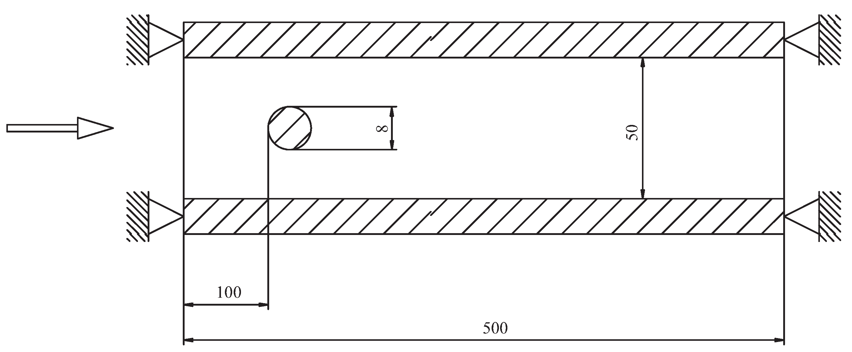
The internal diameter of the channel is d = 50 mm. Wall thickness is h = 5 mm, and length of the channel is L = 500 mm. The density of water is ρ = 998.5 kg/m³. Kinematic viscosity of water is ν = 1.003 · 10⁻³ m/s². The pipe ends are fixed (Figure 1). The diameter of cylinder is d_c = 8 mm. The cylinder is located at l₁ = 0.1 m from the inlet. The inlet water velocity is V = 5 m/s. Relative pressure at the outlet is zero. In the solution of the CFD problem, the pipe walls are stationary. No-slip and no-penetration boundary conditions are applied to the walls. Air pressure and temperature are p = 10⁵ Pa and T = 300 K. Material of the pipe is steel. When calculating the vibro-acoustic problem on the inner walls of the pipe, the pressure fluctuations (pressure amplitudes for each frequency after the Fourier transform) are interpolated from the hydrodynamic problem.

5. Estimations of Flow Quantities

The flow regime is defined by the Reynolds number ${\mathrm{Re}}_h=\rho V{d}_h/\mu$, where $\rho$ is density, V is flow velocity, $d_h$ is hydraulic diameter, $\mu$ is dynamic viscosity. If the flow velocity is $V=5$ m/s, the Reynolds number equals ${\mathrm{Re}}_h=248,804$ (turbulent regime of flow).

In fluid flows past a cylinder, the vortex shedding frequency depends on the Reynolds number [10,11,12]. The Strouhal number is found as $\mathrm{St}=f{d}_c/V$, where f is characteristic frequency, $d_c$ is cylinder diameter, V is flow velocity. The Reynolds number calculated from the cylinder diameter is ${\mathrm{Re}}_c=\mathrm{39,809}$ (turbulent regime of flow). For Reynolds numbers larger than about 1000, the Strouhal number remains almost constant ($\mathrm{St}=0.21$). The vortex street during the flow in a pipe with a cylinder is the dominant non-stationary process; therefore, the fundamental frequency is approximately equal to $f_m=\mathrm{St}V/d_c=131$ Hz, and the oscillation period is $T_m=7.62\times {10}^{-3}$ s.

To describe a periodic process, it is necessary to measure at least two points per period (Nyquist’s theorem). The calculations use approximately 100 points per period to resolve the dominant frequency. The time step is chosen equal to $\Delta t=T_m/100=7.62\times {10}^{-5}$ s. In this case, processes with frequency $f_{\max }=1/(10\Delta t)=1312$ Hz are calculated with 10 points per period.

To perform a Fourier transform on the fundamental tone of a signal, it is necessary to have data for a certain number of periods of this tone. A total of 100 periods of the pitch signal is stored in the calculations. After the oscillations reach a stable mode, the data are saved for $t_f=100T_m=0.76$ s. In this case, it is necessary to perform $N=t_f/\Delta t={10}^4$ steps in time. During the time $t_f$, there are 10 periods with frequency $f_{\min }=10/t_f=12.5$ Hz. Proper resolution is observed in the frequency range from $f_{\min }$ to $f_{\max }$ (greater errors occur above or below these frequencies).

6. Scheme of Simulation

The delayed detached-eddy simulation (DDES) method with a shear stress transport (SST) k–$\omega$ turbulence model is used to resolve vortex structures. DDES is an alternative to Reynolds-averaged Navier–Stokes (RANS) equations and large-eddy simulation (LES). RANS models are not capable of providing acceptable accuracy for calculating flows with large separation zones [7], and LES imposes high requirements on computational resources when modelling separated flows, which makes their practical use difficult [19].

The following approach is used to simulate the unsteady flowfield. A preliminary stationary calculation of the flow in the pipe is performed using the RANS equations with the SST-model. The semi-implicit method for pressure-linked equations-consistent (SIMPLEC) method is used to integrate the equations. Then, unsteady calculations of the flow in the pipe are performed with DDES and the SST-model. The calculations are carried out until a steady state flow is realized. To integrate the equations of motion, a modified pressure implicit with a splitting of operator (PISO) method is used. The pressure correction step is performed more times by the SIMPLEC method. The time step is found from the stability conditions. An unsteady flowfield in a pipe with a fixed time step is found. The pressure values are preserved in each cell bordering the pipe and cylinder walls at every time step.

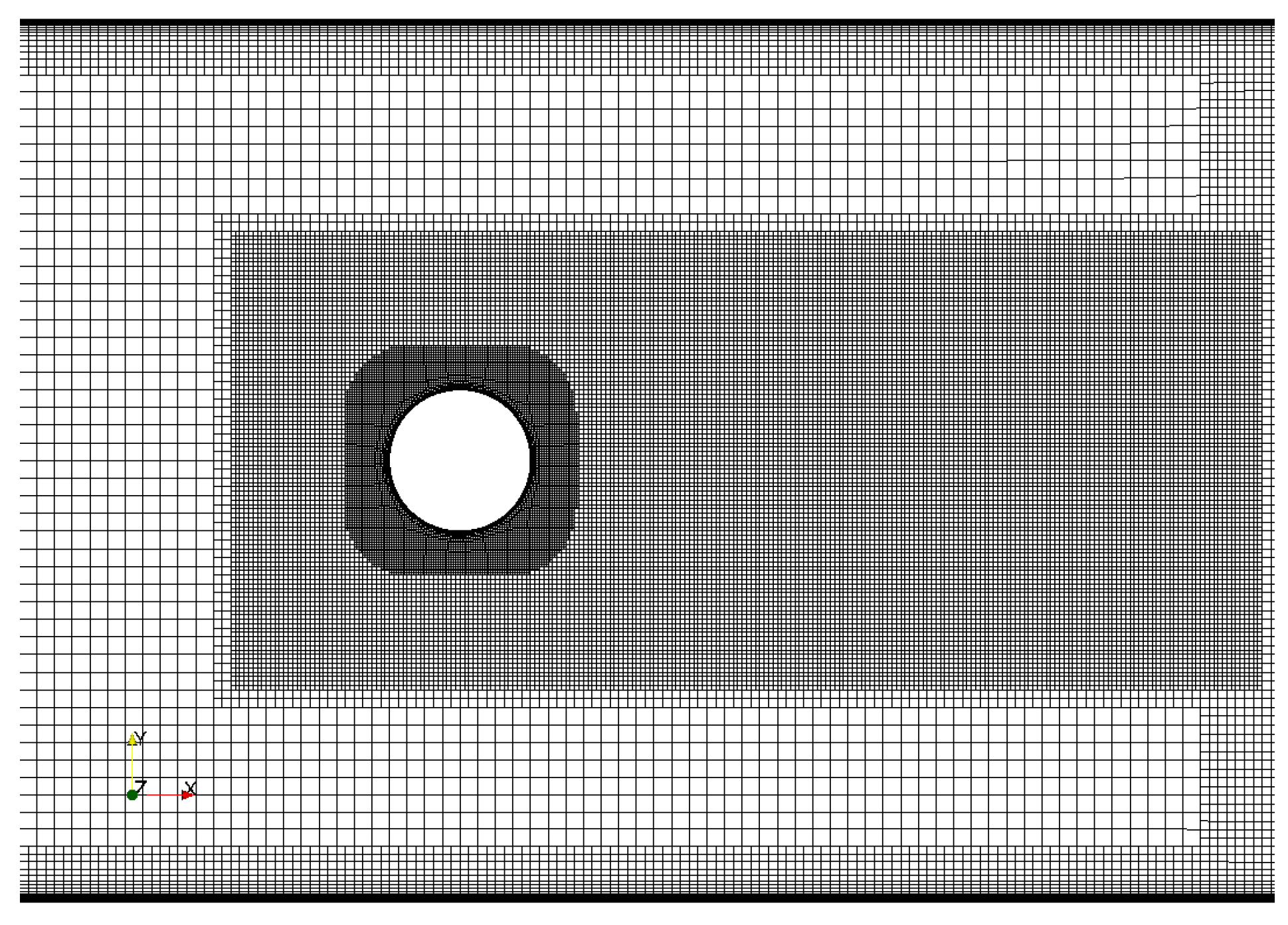
A block-structured mesh is used. Nodes are clustered near the cylinder surface, wake region, and pipe walls to resolve the boundary layer (Figure 2). In the pipe, DDES operates in the LES mode, and the mesh is uniform. In the DDES approach, inviscid fluxes are discretized with a hybrid scheme and the Roe method to maintain accuracy in the LES region and stability of the scheme in the RANS region with a non-uniform and coarse mesh. The distributions of flow quantities found from the RANS solution with the SST-model are used as initial conditions.

The mesh nodes are distributed uniformly along the circumferential coordinate. In the inner region ($0.5⩽r⩽5$), which is a circle, an O-type mesh is used. In the near-wall region ($0.5⩽r⩽1$), the minimum step along the radial coordinate is $r_{\min }=0.003$, the growth factor is $q=1.032$ (about 16 nodes along the radial coordinate are used to resolve the boundary layer). In the outer region, the minimum step in radial direction is $r_{\min }=0.2$, and the growth factor is $q=1.04$. In the buffer region, which is located at a considerable distance from the cylinder and allows avoiding the reflection of sound waves from the boundaries of the computational domain, the maximum step in radial direction is $r_{\min }=20$, and the growth factor is $q=1.09$.

The total number of mesh nodes is about 1.5 million. In this case, the condition $y^{+}<1.2$ is satisfied in the near-wall region. The dimensionless time step is 0.1056. The calculations are carried out on a time interval equal to 162.

Calculations are based on a fully compressible solver [34]. Convergence to a steady state is accelerated by the use of multigrid techniques, and by the application of block-Jacobi preconditioning for high-speed flows, with a separate low Mach number preconditioning method for use with low-speed flows.

With a known flowfield, the calculations of pressure fluctuations that occur on the channel walls due to the influence of an unsteady fluid flow are performed. The boundary condition is set in the form of a known amplitude of pressure fluctuations for each frequency.

The fast Fourier transformation (FFT) allows to obtain dependencies of pressure on time over the pipe walls and cylinder. The data obtained are input for solving the vibro-acoustic problem. The solution of the fluid problem, which describes the distribution of amplitudes of pressure fluctuations along the walls of the pipe and cylinder, contains data with a fine frequency step. For vibro-acoustic calculation, such a set of frequencies is redundant, and therefore, the data are averaged over a coarser frequency grid ($1/n$ octave spectrum filters). The most common are 1/3-octave and 1/8-octave filters.

7. Flow around Cylinder

A numerical simulation of an unsteady flow of a viscous compressible fluid around a cylinder is considered. The calculation results are given for two Reynolds numbers equal to $\mathrm{Re}=150$ (regime 1) and $\mathrm{Re}=3900$ (regime 2), which are widely used for testing numerical methods in the literature. In both cases, the Mach number is set equal to $\mathrm{M}=0.2$. The Reynolds numbers correspond to the flow regime near the cylinder with flow separation from its surface. Using the fast Fourier transform, the values of the Strouhal numbers, the amplitudes of oscillations of the aerodynamic coefficients are determined, and the phases of the formation of vortices and separation of the flow are found from the values of the maximum amplitudes.

7.1. Computational Domain and Boundary Conditions

A transverse flow around a circular cylinder located in a viscous compressible gas, which is at rest for $t⩽0$, is simulated. For $t>0$, the gas is set in motion with a constant speed $U_0$. When calculating the Reynolds number, the diameter of the cylinder and the velocity of the undisturbed flow are used as characteristic parameters of the problem. The equations are solved in the region external to the cylinder boundary.

The center of the cylinder with diameter D is located at the origin. In the $(x,y)$ plane, the computational domain has the shape of a rectangle ($-20<x<80$, $-20<y<20$). The extent of the computational domain in the direction of the z axis is $4D$.

The potential flow field is used as the initial conditions, which is modified in the boundary layer region in such a way as to satisfy the no-slip conditions on the cylinder surface. At the inlet boundary, the velocity of the undisturbed flow is set, which is found from the given Reynolds number, and the temperature is equal to 290 K. At the outlet boundary of the computational domain, non-reflecting boundary conditions are used. A static pressure equal to ${10}^5$ Pa is fixed at the upper and lower boundaries of the computational domain. The surface of the cylinder is assumed to be thermally insulated. In the direction of the z axis, periodic boundary conditions are applied.

7.2. Regime 1

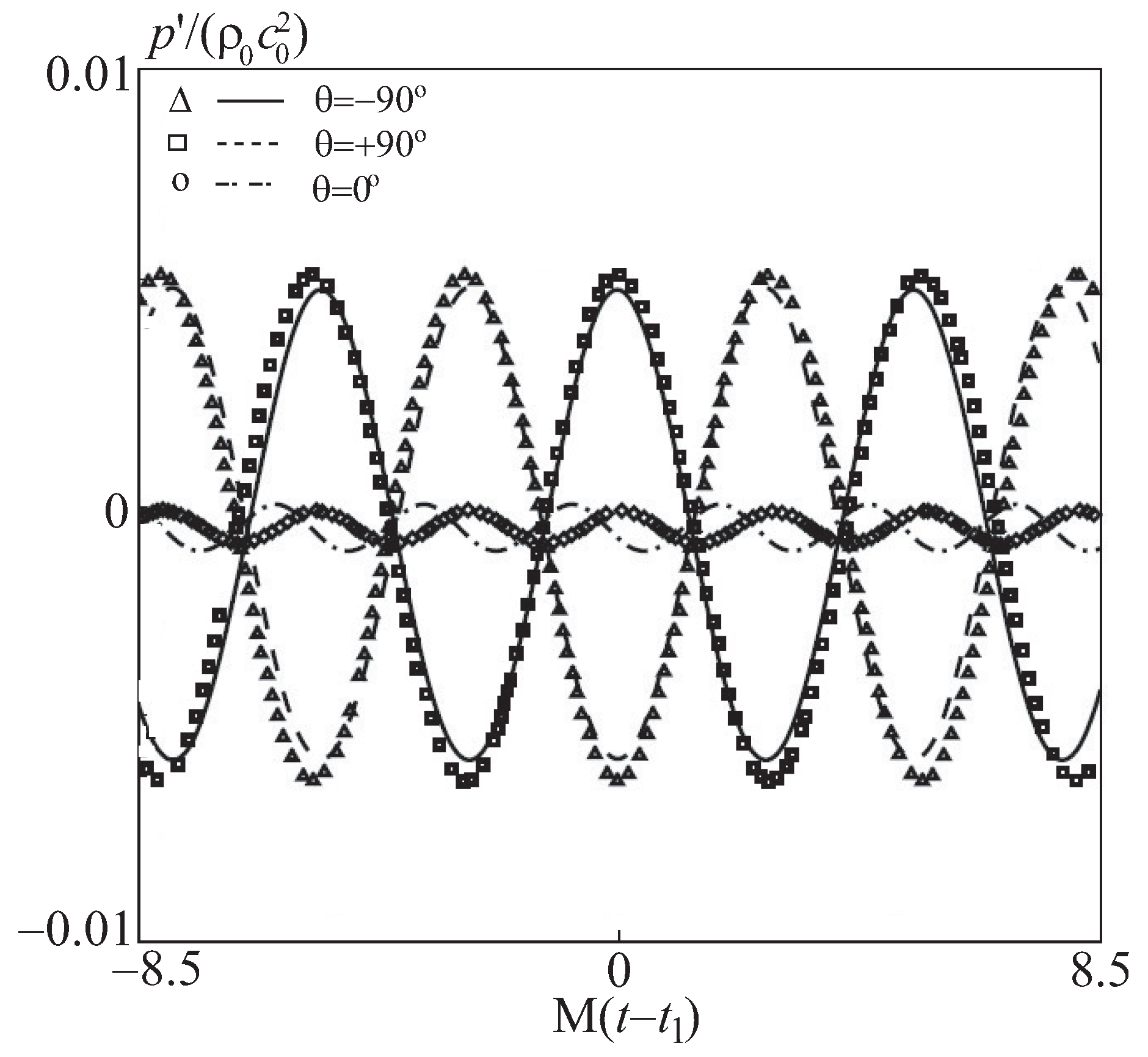
The distribution of pressure over time at various points on the surface of the cylinder is shown in Figure 3. The lines correspond to the numerical simulation data, and the symbols correspond to the calculated data of [10]. There is a fairly good agreement between the calculation results and the data of [10]. The amplitude of pressure fluctuations at $\theta =-90°$ (symbols △, solid line) and $\theta =+{90}^{°}$ (symbols ◻, dotted line) is several times greater than the amplitude pressure fluctuations observed at $\theta =0°$ (symbols ♢, dash-dotted line).

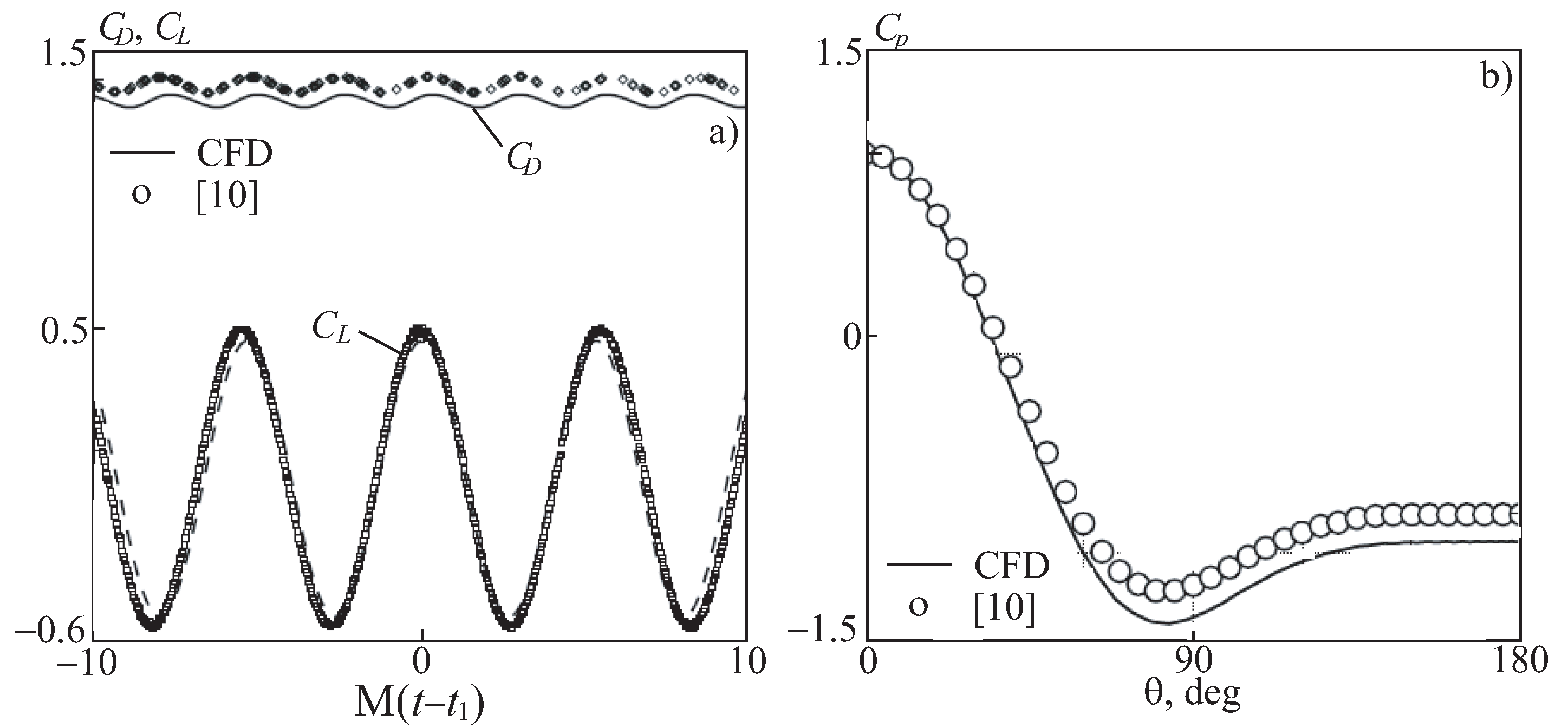
The distributions of the lift coefficient, drag coefficient, and pressure coefficient are shown in Figure 4. The lines correspond to the numerical simulation data, the symbols ∘ correspond to the data of [10]. It achieves good agreement with the available data for all characteristics.

The characteristics of the flow in regime 1 are in good agreement with the available numerical and experimental data (

Table 1. Comparison of calculated data with available numerical and experimental results (for $\mathrm{Re}=150$).

Source	St	$-{\overline{\mathit{C}}}_{\mathbf{pb}}$	${\mathit{C}}_{\mathit{L}}$	${\mathit{C}}_{\mathit{D}}$	${\mathit{L}}_{\mathit{z}}/\mathit{D}$
CFD	0.186	0.850	0.342	1.224	20
[18]	0.184	0.848	—	1.313	140
[13]	0.185	0.885	—	1.333	56
[16]	0.181	—	0.338	1.268	16.46
[14]	0.191	—	0.403	1.418	12
[12]	0.183	—	0.356	—	—
[8]	0.184	0.856	—	—	—
[10]	0.184	—	—	1.334	—
[20]	0.184	0.846	0.355	1.305	—

, where $C_{pb}$, $C_L$, and $C_D$ are the mean pressure coefficient, the mean square lift coefficient, and the mean drag coefficient). In particular, in calculations the Strouhal number is 0.186, while the data of a physical experiment give a value of 0.184 [8] and 0.183 [12]. The angular coordinate of the flow separation point is ${\theta }_s=108.5°$. Averaging is carried out over a time interval equal to 150. To find the Strouhal number, the correlation relation $\mathrm{St}=0.2684-1.0356{\mathrm{Re}}^{-1/2}$ from [15] is used. 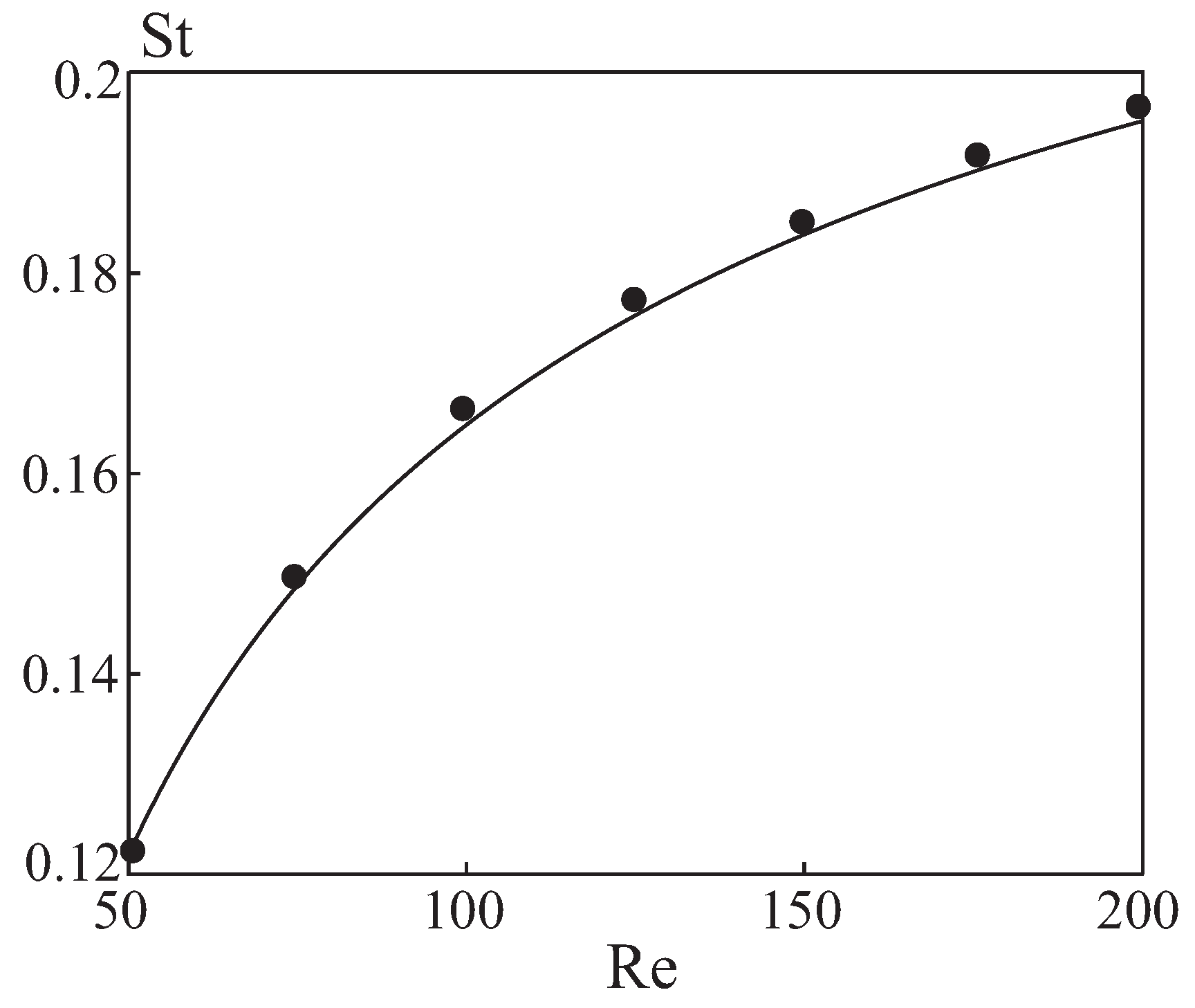The Strouhal number equals $\mathrm{St}=0.1838$ for $\mathrm{Re}=150$, which is in good agreement with the obtained value. The results of calculations of the Strouhal number in comparison with experimental data are shown in Figure 5.

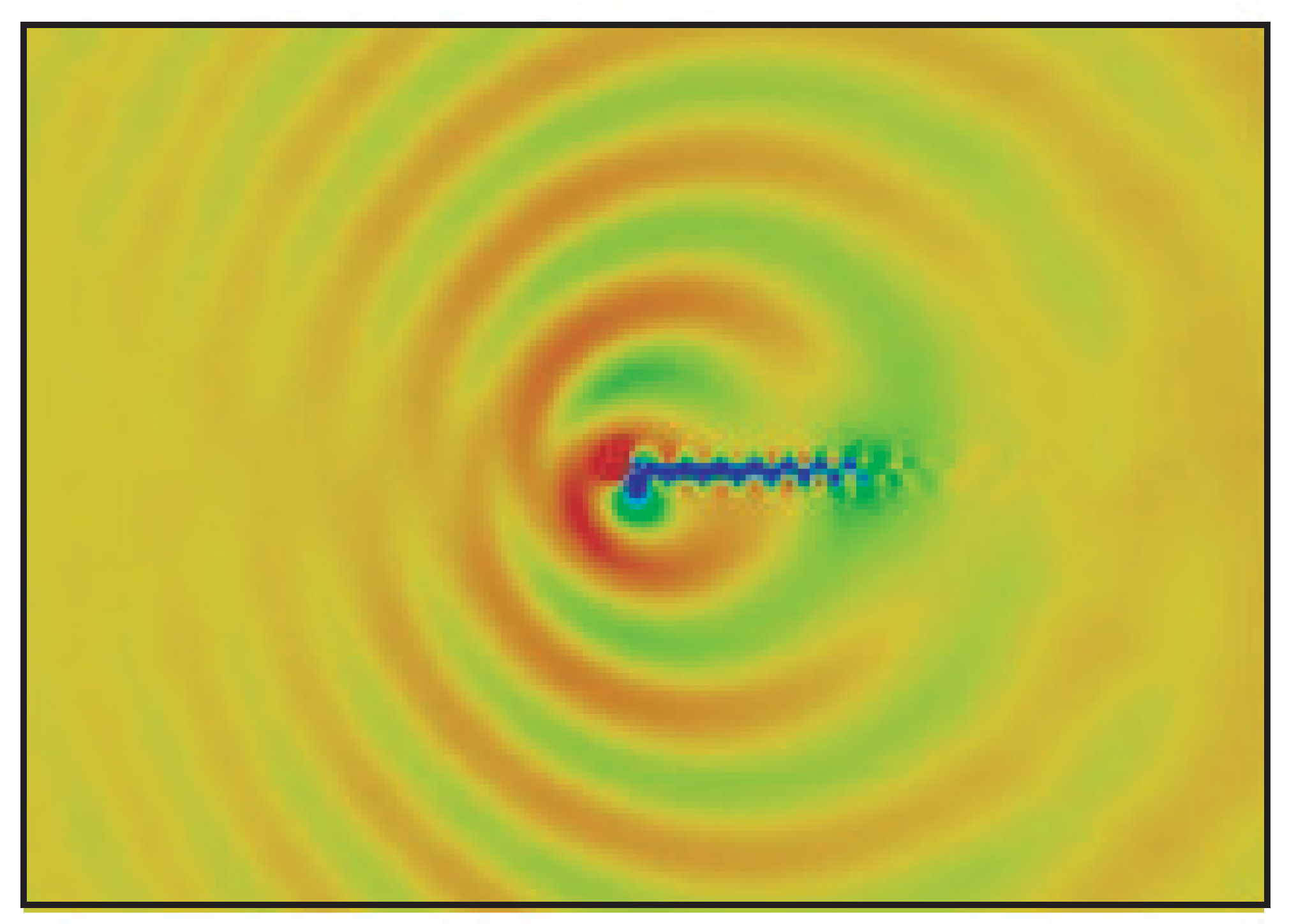
The instantaneous pressure distribution near a circular cylinder is shown in Figure 6, which clearly shows oscillations of the wake behind the cylinder.

7.3. Regime 2

The characteristics of the flow in mode 2 are in good agreement with the available numerical and experimental data (

Table 2. Comparison of calculated data with available numerical and experimental results (for $\mathrm{Re}=3900$.

Source	St	$-{\overline{\mathit{C}}}_{\mathbf{pb}}$	${\mathit{C}}_{\mathit{L}}$	${\mathit{C}}_{\mathit{D}}$	${\overline{\mathit{C}}}_{\mathit{D}}$	${\overline{\mathit{\theta }}}_{\mathit{s}}$	${\mathit{L}}_{\mathit{r}}/\mathit{D}$	${\mathit{L}}_{\mathit{z}}/\mathit{D}$
CFD	0.209	0.860	0.074	0.029	0.963	88.3	1.57	20
[17]	0.219	0.840	—	—	—	—	1.59	20
[19]	0.220	0.920	—	—	1.03	85.7	1.30	18

). $C_{pb}$, $C_L$, $C_D$, ${\overline{C}}_D$, ${\theta }_s$ are understood as mean pressure coefficient, mean square lift coefficient, mean square drag coefficient, mean drag coefficient, mean angular coordinate of the lift-off point, average length of the recirculation region. In particular, in the calculations, the Strouhal number is 0.186, while the data of a physical experiment give values of 0.184 [8] and 0.183 [12]. The angular coordinate of the flow separation point is ${\theta }_s=108.5°$. Averaging is carried out over a time interval equal to 150.

The cause of noise generation is the deterministic tone sound with discrete frequencies and turbulent fluctuations in the boundary layer and wake, which are stochastic in nature and have a continuous frequency spectrum. The sound intensity is found from the relation $I=\overline{p^{\prime 2}}/\left({\rho }_0{c}_0\right)$. The RMS pressure is determined by the relation

$$\begin{array}{c}\hfill 〈p^{\prime 2}\left(\mathbf{x}\right)〉=\underset{T\to \infty }{lim}\frac{1}{T}\underset{0}{\overset{T}{\int }}{p}^{\prime 2}(\mathbf{x},t)dt,\end{array}$$

where $T=t_n-t_0$ is the averaging period. Under $t_0$ and $t_n$, we mean the moments of time corresponding to the beginning and end of saving the samples.

RMS pressure distributions obtained using various approaches are shown in Figure 7. The control surface is located at $r_0/R=1.2$, and the observation point—on a circle with radius $r_c/D=250$. Symbols ◻ correspond to simulation results, dash-dotted line—experimental data [12] at $\mathrm{Re}=3000$, double dash-dotted line corresponds to experimental data [12] at $\mathrm{Re}=5100$. Good agreement between the calculated and experimental data takes place at $30<L_c/D<150$.

8. Results and Discussion

The structure of the flow behind a transversely streamlined cylinder in a stationary external flow has been well studied. In the case of a transverse flow around a cylinder, a boundary layer is formed on its surface, the thickness of which gradually increases upstream. The main determining parameters of this layer are the Reynolds number and the turbulence of the oncoming flow. The separation of the boundary layer and the formation of vortices in the wake of cylindrical bodies are periodic processes. The frequency of separation is characterized by the Strouhal number, which depends on the Reynolds number, the turbulence of the external flow, the degree of obstruction of the channel, and other factors.

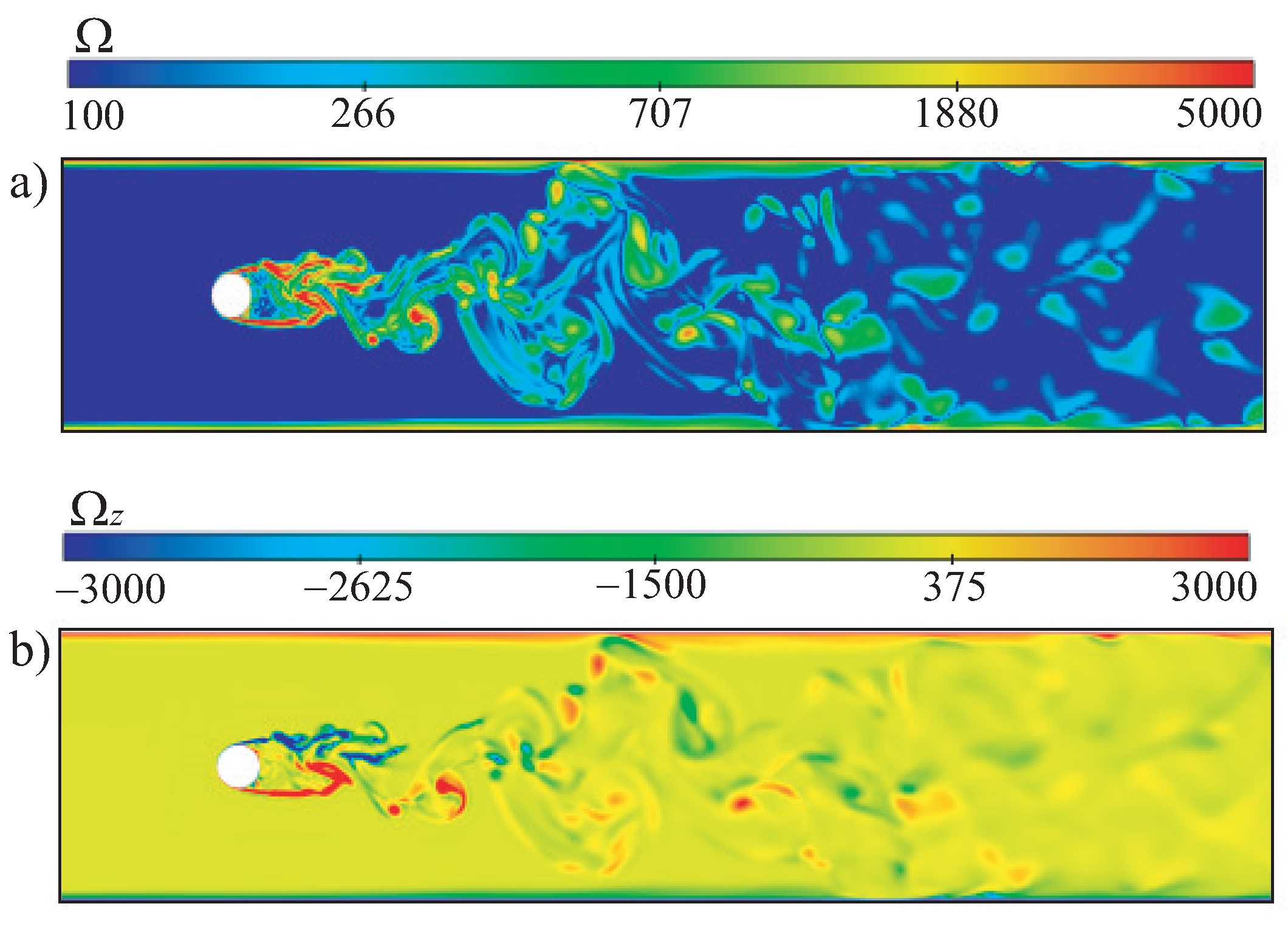
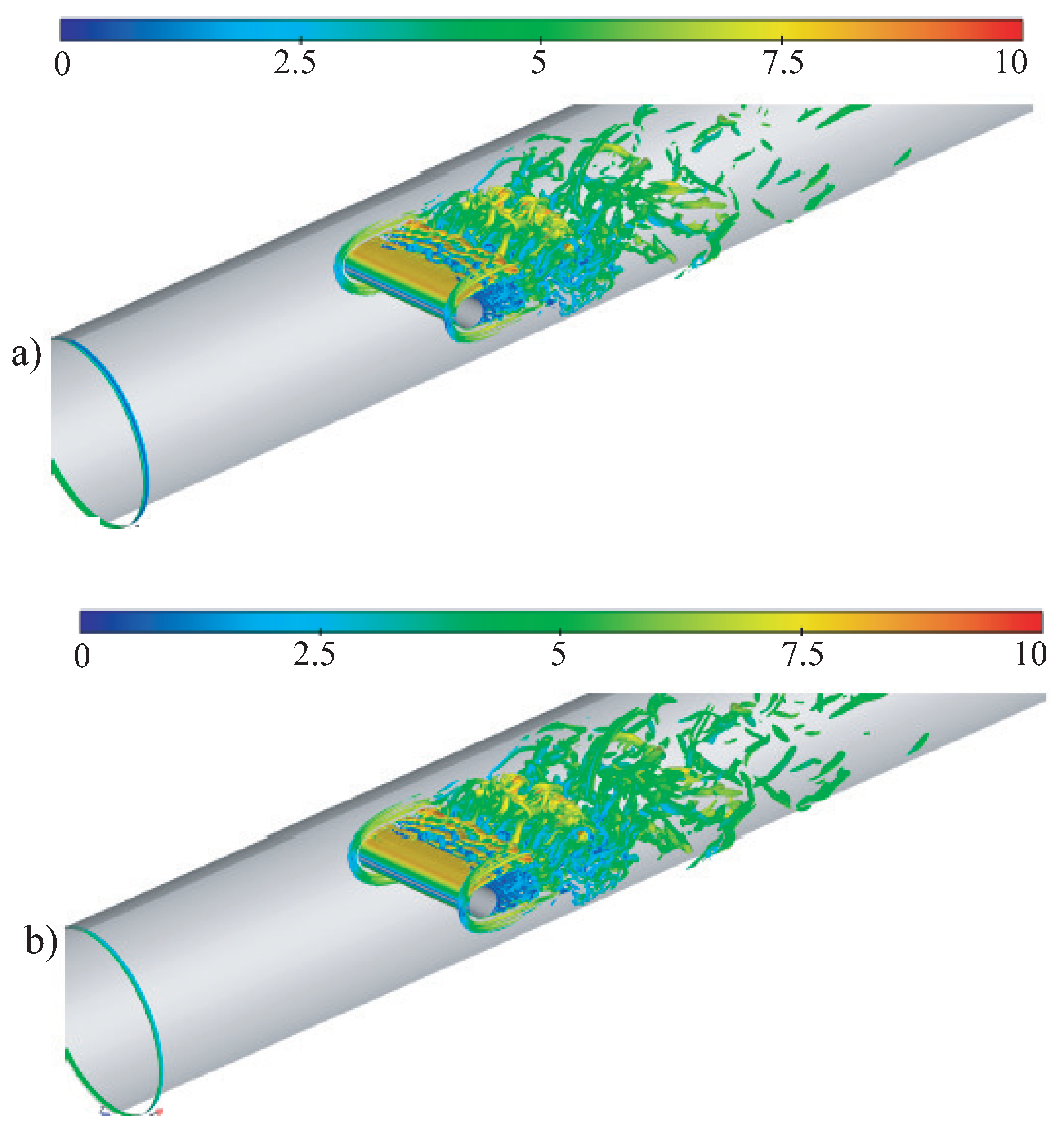
The flow that is formed when the boundary cylinder is separated from the surface loses its stability and interacts with the pipe walls. As a result, self-sustaining pressure oscillations arise, which lead to the presence of intense peaks in the spectrum of the generated noise. The field of the vorticity modulus and the z-component of the vorticity vector in the symmetry plane are shown in Figure 8. The vortices form an extensive wake, grow downstream, and interact with the pipe walls. The level lines of the z-component of the vorticity vector give an idea of the direction of rotation of the vortices.

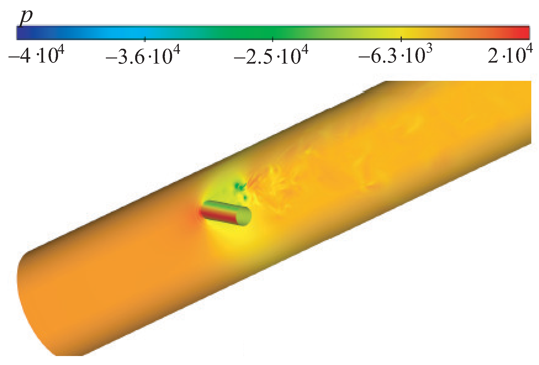
The distribution of overpressure on the channel walls is shown in Figure 9. The pressure is distributed in a significantly non-uniform way, and therefore, one should expect the occurrence of oscillations of the elastic walls of the pipe.

One of the criteria used to identify eddy flows is the Q-criterion

$$\begin{array}{c}\hfill Q=\frac{1}{2}\left({\left|\mathrm{\Omega }\right|}^2-{\left|S\right|}^2\right),\end{array}$$

where $\left|S\right|={\left[\mathrm{trace}\left(S{S}^{\prime }\right)\right]}^{1/2}$, $\left|\mathrm{\Omega }\right|={\left[\mathrm{trace}\left(\mathrm{\Omega }{\mathrm{\Omega }}^{\prime }\right)\right]}^{1/2}$. The tensor invariant is

$$\begin{array}{c}\hfill Q=-\frac{1}{2}\left({\lambda }_1+{\lambda }_2+{\lambda }_3\right),\end{array}$$

where ${\lambda }_i$ are the eigenvalues of the velocity gradient tensor ($i=1,2,3$). A vortex is defined as a flow region in which the inequality $Q>0$ is satisfied (the flow region in which the norm of the vorticity tensor exceeds the norm of the strain rate tensor). The connection between the pressure and the Q criterion is established using the Poisson equation for the pressure ${\nabla }^{2}p=2\rho Q$. The condition $Q>0$ does not necessarily correspond to the pressure maximum (for $Q>0$, the pressure maximum is observed at the boundary).

To identify eddies, the ${\lambda }_2$-criterion is used, based on the decomposition of the velocity gradient tensor into symmetric (strain rate tensor) and antisymmetric (rotation tensor) tensors [35]. The $S^2+{\mathrm{\Omega }}^2$ tensor is symmetric and has real eigenvalues (${\lambda }_1⩾{\lambda }_2⩾{\lambda }_3$), two of which are negative. The vortex flow region is defined as the region in which

$$\begin{array}{c}\hfill {\lambda }_2\left(S^2+{\Omega }^2\right)<0,\end{array}$$

where ${\lambda }_2\left(A\right)$ is an eigenvalue of the symmetric tensor A. Under adiabatic conditions, this criterion guarantees an instantaneous pressure minimum in a two-dimensional flow [36].

The level surfaces of the Q and ${\lambda }_2$ criteria, which are different combinations of the velocity gradient tensor invariants [37], colored according to the value of the velocity modulus, make it possible to visualize the vortex structure of the flow (Figure 10). The figure clearly shows both the three-dimensional flow structure and the resulting large-scale vortex component of the Karman street.

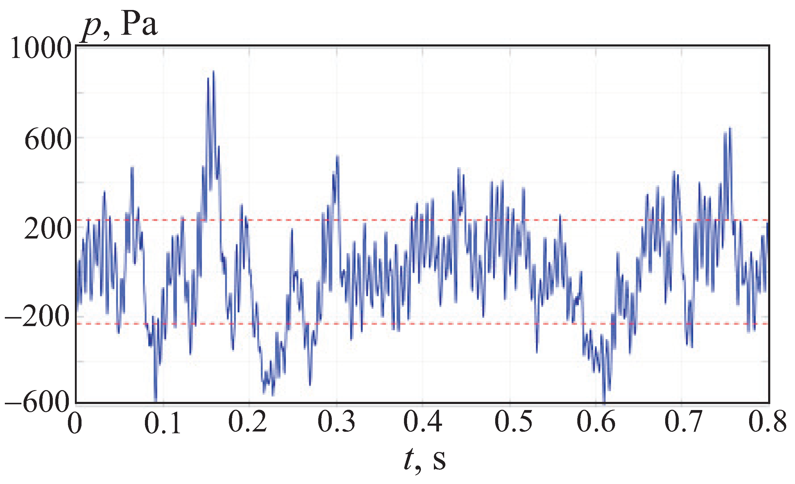
The presented fields of physical quantities illustrate the general picture of the separated flow near the cylinder. As quantitative estimates of the accuracy of solving this problem, the most interesting are the spectra of pressure fluctuations on the cylinder surface and acoustic loads on the pipe walls. At each point on the wall, as well as at some selected points, the Fourier transform of the data is performed, expressing the dependence of pressure on time. The time dependence of overpressure on the pipe wall is shown in Figure 11 at $x=0.1$ m. Dotted lines show pressure levels corresponding to $\pm 200$ Pa.

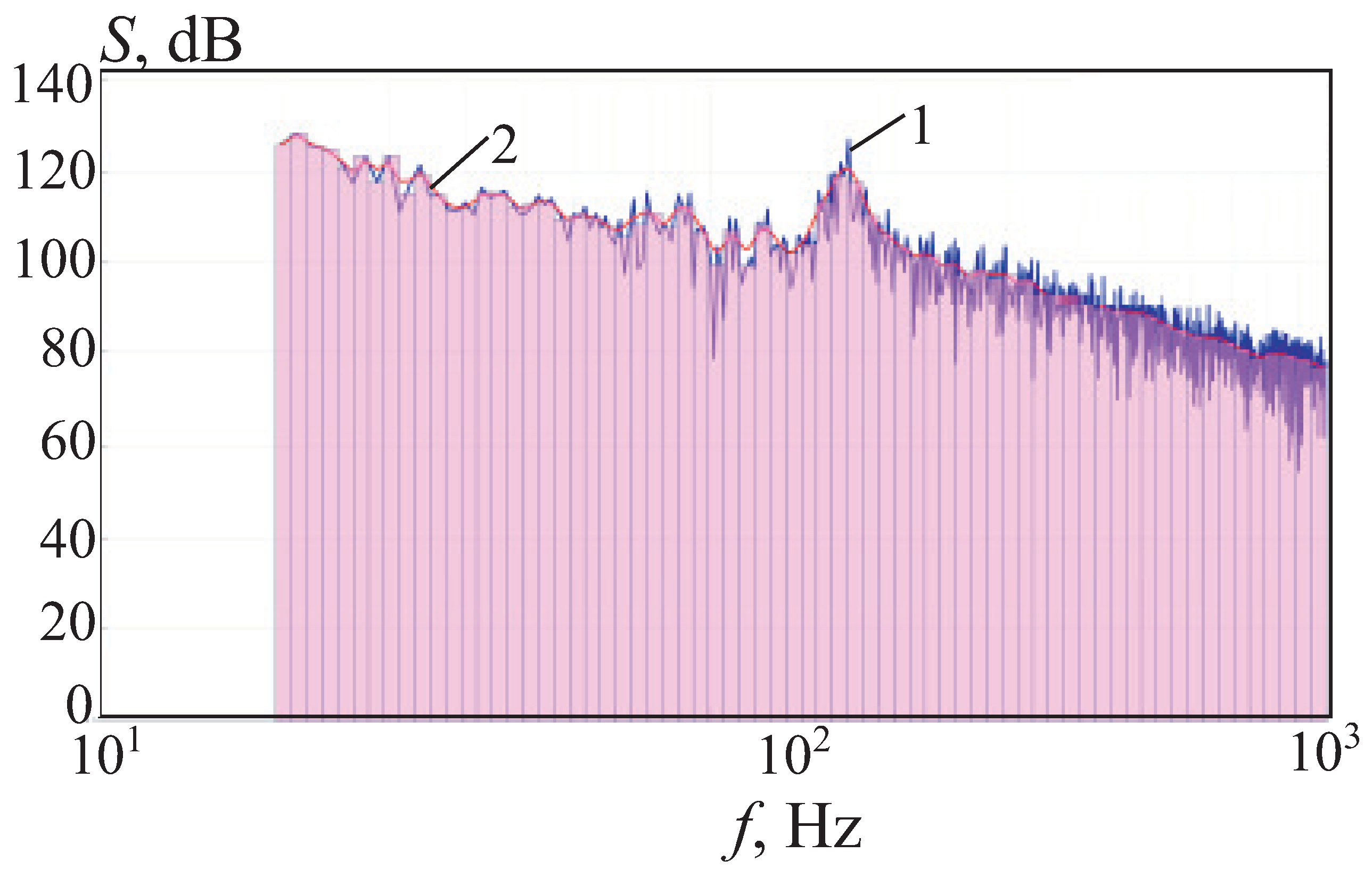
The Fourier transform of the pressure signal at the same point is shown in Figure 12. Line 1 shows the results of calculations, line 2—smoothed spectrum, and columns—results of calculations using the $1/12$ filter. A peak with a frequency corresponding to the fundamental tone of the pulsations stands out well.

The distribution of the spectrum over all points on the channel wall for a certain frequency makes it possible to judge the places of the most intense impact from the flow on the walls at a given frequency (Figure 13).

The power spectral densities of near-wall pressure fluctuations on the streamlined surface and on the channel walls have clear discrete peaks that correspond to the nature of the vortex motion over the surface under study. Discrete peaks of the spectral levels of near-wall pressure fluctuations, which have the most energy-intensive main frequency harmonic, have higher-order harmonics, as well as sub-harmonics, due to the nonlinear interaction of vortex structures (sources of pseudo-sonic fluctuations) with each other and with the surface in a stream. This occurs due to the merging of the vortex structures dominating here with each other (generation of sub-harmonics) and their destruction in accordance with the mechanism of the cascade process of vortex transformation.

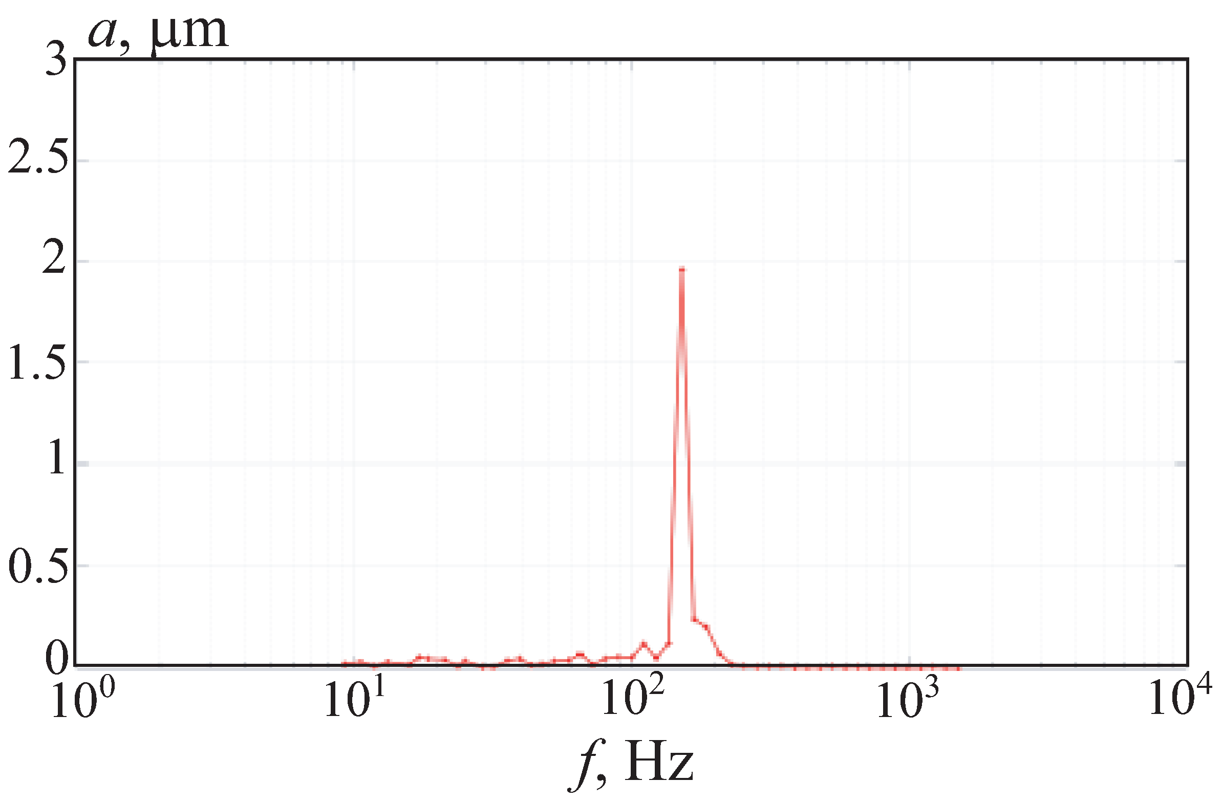
As a result of the calculations, the displacement amplitudes were obtained depending on the frequency. The dependence of the displacement amplitude at the point $(0.5,0,0)$ is shown in Figure 14. There is a clear peak corresponding to the frequency of the fundamental tone.

9. Conclusions

A mathematical model and computational algorithm to perform coupled simulations of unsteady processes in the circular channel with a round cylinder were developed and validated. At the first stage, the velocity and pressure fields are calculated with delayed detached eddy simulation. At the second stage, the problem of calculating the stress–strain state of the pipe is solved using the finite element method.

Stand-alone CFD simulation of unsteady viscous flowfield around a circular cylinder were performed, and results of CFD calculations were validated against experimental and computational data from the literature. The values of Strouhal numbers and amplitudes of oscillations of the aerodynamic coefficients are determined with the fast Fourier transformation technique.

When fluid flow separates from the cylinder and flow loses its stability, self-sustaining pressure oscillations arise, which lead to the presence of intense peaks in the spectrum of the generated noise. The spectrum of pressure oscillations on the cylinder surface and wall of the pipe have clear discrete peaks. The behavior of spectral dependencies is generally preserved if the flow velocity (Reynolds number) increases.