Abstract
The development of energy-efficient solutions for large-scale fermenters demands a deep and comprehensive understanding of hydrodynamic and heat and mass transfer processes. Despite a wide variety of research dedicated to measurements of mass transfer intensity in bubble flows, this research subject faces new challenges due to the topical development of new innovative bioreactor designs. In order to understand the fluid dynamics of the gas–liquid medium, researchers need to develop verified CFD models describing flows in the bioreactor loop using a progressive physical and mathematical apparatus. In the current paper, we represent the results of evaluating the key performance indicator of the bioreactor, namely the volumetric mass transfer coefficient () known as a parameter of dominant importance for the design, operation, scale-up, and optimization of bioreactors, using the developed thermometry method. The thermometry method under consideration was examined within a series of experiments, and a comparative analysis was provided for a number of various regimes also being matched with the classical approaches. The methodology, experiment results, and data verification are given, which allow the evaluation of the effectiveness and prediction of the fluid flows dynamics in bioreactors circuits and ultimately the operational capabilities of the fermenter line.
1. Introduction
Despite the impressive recent development of the practice of applying modern numerical and computational methods to hydrodynamic flow analysis [1,2,3,4,5,6,7,8,9], as well as machine learning methods [10,11,12,13] for modeling, analyzing, and evaluating the performance parameters of various engineering solutions in the field of fermentation [14,15], a number of questions remain as an open challenge for the scientific community [16,17,18]. Among them lies a fair assessment of fermenters’ performance indicators [19,20,21] for the case of the large-scale transition from laboratory to industrial solutions. Another indisputable challenge for researchers in the field of biotechnology is the development and implementation of analytical modules for the control system of mass transfer characteristics of the fermentation process [22,23,24,25]. Both of these problems require an adequate verified description of the behavior of bubbles in a two-phase gas–liquid medium of a bioreactor [26,27,28,29], in particular, the development of relevant experiments and methods for evaluating the mass transfer in the system [14,30,31,32]. The latter is particularly relevant since, together with the energy consumption associated with the fermenter’s performance and therefore the direct economic effect when choosing the bioreactors types, the () coefficient must be measured by methods that do not involve shutting down the fermentation process at the plant and, moreover, do not require any sort of chemical interventions in the circuit of the plant (as, e.g., i is assumed in the case of a number of classical approaches such as the sulfite method). Thus, the requirements of maximum non-interference in the fermentation process, the need to carry out measurements in parallel with the main (complicated microbiological) processes, and reasonable considerations regarding the final cost of resources for such regular measurements lead researchers to the need to find new methods that meet the above claims. The present study is devoted to solving the aforementioned problem based on a sample stand of a mass transfer apparatus designed for the process of growing microorganisms on various types of substrates [9,26,33], namely a jet bioreactor with the recirculation of liquid and gas phases of an air–water and air–model liquid of a given rheology system. Studied experimentally on various scales of plantsand evaluated critically from the point of view of compliance with the results of other measurement methods, the presented thermometric method was proven indeed to be a promising tool for measuring the efficiency in mass transfer apparatuses, including large-scale (in our experiment, up to 1000 cubic meters) fermentation plants. An experimental study of the life-cycle analysis of bubbles, its evolution, and mass transfer characteristics in jet bioreactors (when mixing is carried out due to a falling jet of liquid initiated by pump operation) was provided when the bubbles passed through a closed circuit of the fermenter. The experimental module was designed in order to include a set up wide enough to evaluate hydrodynamics and calculate the mass-transfer parameters of the fermenter depending on the performance of the circulation pump, the amount of air supplied, and the degree of filling of the apparatus circuit etc. The thermometry method for volumetric mass transfer coefficient () evaluation based on the transition of the mechanical form of energy into heat due to the operation of the pump [34] was investigated and verified in particular with sulfite method and calculations performed on the basis of input mechanical energy. We have also focused on investigating the limits of applicability of these methods for various operating modes and scales of experimental setup, investigating the influence of concrete numerical values and corridors of input parameters on the behavior of gas–liquid flows.
2. Materials and Methods
2.1. Theory of the Thermometry Method
The cornerstone of the fermentation process, namely the aforementioned calculation of the volumetric mass transfer rate, depends directly on the type of installation (fermenter) that provides the gas–liquid fluid flow transition. One knows a number of various empirical formulas for determining the dissolution of gas (oxygen) for bubbling, bubbling-airlift, gas-lift, nozzle gas distribution [35], and finally jet units, which are considered in the current manuscript. At least two main, physically natural, parameters in these formulas are worth mentioning, namely (1) specific input energy (power) spent on mixing and aeration , kW/m, since diffusion processes in a liquid are intensified with an increase in the Reynolds number in terms of the relative velocity of the liquid and gas phases [36], and thus the energy dissipation of the gas flow was carried out as a result of the work of the gas flow against friction velocity, and (2) and true volumetric gas fraction (void fraction) . The volumetric gas fraction in the apparatus could thus be defined as the ratio of the volume of the gas phase to the volume of the gas–liquid mixture. As increases, the specific interfacial surface also increases. In a particular idealized case, e.g., in a monodisperse bubble medium, the interfacial area per unit volume is equal to D, where D is the gas-bubble diameter. This fact can be explained by an example. Let us denote as bubble volume. The number of bubbles per unit volume , and the total area of the interfacial surface per unit volume . When designing a jet fermenter of an overflow type, the ratio of the volume of the gas phase to the volume of the gas–liquid mixture is taken to be equal to . We also take into account [34] the following formula outflow for the definition:
where , and are coefficients assigned specifically for the type of apparatus under consideration. In jet fermenters, when mixing is provided through the falling jet of liquid caused by the operation of the pump, with natural ejection of the gas by a liquid jet, the mass transfer coefficient in the liquid phase is thus proposed to be calculated using the following formula [37]:
The specific input power spent on mixing and aeration represents itself as the mechanical (useful) power of the rotary pump. It should be noted that in real experiments, the calculated power consumption of the pump might differ significantly from since asynchronous motors are widely in use for pump operation and thus the efficiency depends on the load lying in practice from to . In other words, considering that equal to the measured power consumption appears to be incorrect, and taking into account [38], is rather spent on the following:
- 1.
- Averaged and turbulent (pulsation) kinetic energy of the flow,
- 2.
- Change in the potential energy of the fluid in the gravitational field,
- 3.
- Enthalpy change (heating of liquid due to thermal dissipation),
- 4.
- Heat of gas dissolution (negative),
- 5.
- External heat losses of the circuit,
- 6.
- Interfacial “liquid–gas” energy.
In stationary (quasi-stationary) modes of operation of the closed circuit of the bioreactor, the kinetic and potential energies of the flow (1 and 2) do not change. If one neglects the heat of condensation and heat losses (4 and 5), the specific input power for mixing the medium in the apparatus might be calculated as follows:
where C is the specific heat of the liquid (the heat capacity of the apparatus walls is considered negligible). Expression denotes liquid temperature difference during the determination time, and is the relative measurement period.
It is worth mentioning that when thermometry method is applied, it is crucial to make the first measurement of the temperatures when achieving the steady flow regime. In turn, this is determined by the time of establishment of the stationary turbulent spectrum in the flow. For regular contour sizes (internal diameters of pipes are centimeters or tens of centimeters) and Reynolds number (tens or hundreds of thousands, which corresponds to developed turbulent regime), this time is on the order of a few seconds. During this time period, the “gas–liquid” interfacial surface most likely formed.
In general, this formula can be modified in cases when significant external heat losses or significant heat of dissolution takes place. If the circuit is not closed and during the circulation of the liquid a complete or partial renewal of the liquid takes place, it is obligatory to take into account the change in the kinetic and potential energy of the flow, as well as the change in the interfacial surface since the intake and removal of fluid can be carried out at various speeds and on various heights, a new interfacial surface is additionally formed. Finally, with a constant gas supply, it is necessary to take into account its excess enthalpy, which is meanwhile partially expended on the gas dissolution. According to the assessment, the external heat losses of the circuit make a significant contribution to determining the specific input power since the surface of the apparatus is extensive and not thermally isolated:
where [W/m] represents total coefficient of heat transfer by radiation and convection; is responsible for heat exchange surface area of the apparatus, and for its surface temperature. Accordingly, corresponds to ambient temperature.
2.2. Design and Procedure of the Experiment
Verification of the thermometric method was carried out on the developed experimental setup (Figure 1), designed especially to recreate the complete operation of a jet ejection bioreactor with a working volume of 0.1 in terms of hydrodynamic flows. The setup is represented as a closed hydrodynamic circuit with free input for the gas phase injections. For additional verification and comparative analysis of the range of applicability of various methods for measurement, the archive data were used for the analogous setup of a similar design type, but eight times bigger by working volume than the main experimental setup (see also Section 3 ).
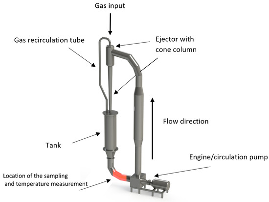
Figure 1.
Experimental setup for measuring the mass transfer of the air–liquid flow. The design of the experimental setup corresponds to the real field jet bioreactor for manufacturing the microbiological single-cell protein and corresponding high-added-value products.
The principle of operation of the designed experimental setup is shown on Figure 1. The motor rotates the circulation pump, which ensures the rise of liquid through the circulation circuit into the overflow ejector. Once in the ejector, the liquid, subjected to gravitational force, falls into the tank, entraining the air through the inlet valve, as well as from the recirculation tube connecting the tank and the ejector. The device absorbs the air up to a state of saturation. Meanwhile, in the ejection column, a bubbly medium is formed, which provides the most intensive mass transfer and saturation of the liquid with dissolved gas. During the operation, the experimental setup is controlled by a single parameter: the pressure-flow characteristic of the pump, determined by the consumed energy of the engine. The tactical task of the planned experiments was to determine the rate of oxygen dissolution, as well as to calculate the volumetric mass transfer coefficient. The experiments were carried out for the media characteristics represented in Table 1.

Table 1.
Experimental media and hydrodynamic regimes parameters.
The above-mentioned special model liquid was determined as a mixture of water and glycerin at a ratio of 11.5:1. Such a fluid satisfactorily models the rheology of a biological fluid used in industrial bioreactors [9]. On the initial phase, the experimental setup was filled with liquid up to a working volume of m and preheated up to the ambient (air) temperature. Then, the pump was started, and the experimental setup was saturated with air (air absorption in the ejector then stops), and the procedure of temperature measurement of the liquid in front of the pump was initialized (see Figure 1). The measurement series were made accurately every 300 s using a GMH 3230 digital high-precision, low-inertia thermometer. The results of thermometric measurements, namely the dependence of water temperature on time for various pump operation modes, are shown in Figure 2. The corresponding specific volumetric power values on the pump impeller for these modes are given in the figure’s legend. The graph shows that a greater specific input power corresponds to a greater slope of the graph. Accordingly, larger angles of inclination correspond to larger thermal outputs.
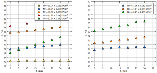
Figure 2.
Relative temperature of the liquid changes with time, thermometry method applied on water (left) and model liquid (right).
In order to determine the reasonably applicable intervals of the thermometric method, as well as to confirm the relevance of the obtained absolute values measured and calculated, the sulfite method of measurement of the the intensity of oxygen dissolution in water [39,40,41,42] was used as a reference. The choice of the sulfite method for studying mass transfer in the liquid phase was determined due to the fact that the oxidation reaction of sodium sulfite occurs in the bulk of the liquid, and the process of chemisorption of air oxygen by an aqueous solution of sodium sulfite is determined by the diffusion of oxygen in the liquid boundary film. Since the resistance in the gas phase is negligible, the entire process of sodium sulfite oxidation is limited by mass transfer in the liquid phase. An aqueous solution of copper sulfate with a concentration of more than 10 kmol/m at a concentration in a solution lies within the range of depending on the quality of mass transfer (the higher the rate of dissolution of oxygen, the more we take the concentration for the accuracy of determination due to the measurement technique). According to a number of researchers [37], the rate of a chemical reaction in the presence of copper ions does not depend on the concentration of sodium sulfite. The latter makes it possible to neglect the degree of mixing of the liquid when calculating the driving force of the process. In the presence of a catalyst, the reaction proceeds in the diffusion region, where the rate of sulfite oxidation is limited by the resistance in the liquid phase, so the core of the sulfite method is based on the oxidation reaction of sodium sulfite in the presence of a catalyst—copper or cobalt ions: . The excess sulfite remaining is determined by iodometric back-titration [39,41]. Sulfite concentrations applied range from n up to 1 n. Note that the rate of the chemical reaction of sulfite oxidation is much higher than the rate of absorption, so the overall rate of the process is determined by the rate of absorption. The sulfite coefficient (sulfite number) determined by this method characterizes the rate of oxygen absorption in the experimental setup (normal range is from to 5 and rarely reaches 10 mmol/L min for . Parameter might be determined by the physical–chemical properties of the sulfite solution and the hydrodynamic parameters of the system. Since the reaction between dissolved oxygen and sulfite is close to instantaneous and the concentration of dissolved oxygen is zero, we have:
It is worth mentioning that normally the value, determined by the sulfite method, is higher than what might be determined by the direct method [37,40,42]. The experimental setup was filled with liquid up to a working volume of , heated preliminarily up to the ambient (air) temperature; the pump was started, and the process of sampling from the line in the position in front of the pump was begun (see Figure 1). Sampling was carried out every 180 s, and each iteration demanded sample volume as of 50 mL of liquid. The results of the measurements of sulfite spent for the titration are represented on Figure 3.
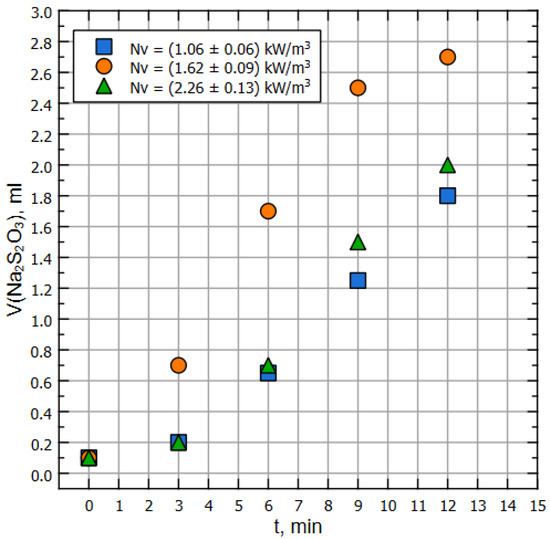
Figure 3.
Amount of thiosulfite used for titration, mL per minute.
Note that for both of Figure 2 and Figure 3, dots of the same color correspond to the same pump’s RPM, but the specific power on the impeller is different due to the properties of the liquids (water and model liquid).
The sulfite M number can be determined according to the formula [37,40,42] (aa), where: is experience exposure and a and a are final and initial amount of N solution of sodium hyposulfite spent for the titration. Typically, the time intervals with the highest sulfite consumption are used [40,42]. Finally, the mass transfer coefficient in the liquid phase was determined by the ratio , where is equilibrium oxygen concentration in relation to the gas phase ( mg/L, kg/m is taken for calculations) for the experimental conditions; is the concentration of oxygen dissolved in the liquid, equal to zero in our case; £ is the coefficient of acceleration of the process of oxygen chemisorption in relation to biosorption , and this coefficient is taken based on the design of the fermenter.
3. Results
Figure 4 shows the dependence of on for various liquids (water and special model liquid) and methods for measurements on the experimental setup designed in strict accordance with real jet-fermentation apparatuses. Note that the measurements were carried out in the steady state mode of heat exchange between the reactor and the environment according to the measurement protocols. In Figure 4, the black curve corresponds to calculated dependence, and blue dots correspond to the data obtained using the thermometric method for the water at different setup regimes (see Table 1); green dots correspond to the data obtained using the thermometric method for the model liquid ( ) at different setup regimes (see Table 1). Finally, red dots represent the data obtained according to the sulfite methodology , with the same regime range.
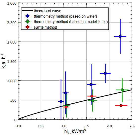
Figure 4.
Dependence of on for various liquids and methods of measuring on an experimental apparatus. The measurements were carried out in the steady state mode of heat exchange between the reactor and the environment according to the measurement protocol.
It should be noted that an increase in engine speed leads to an increase in the specific input power (in the operating frequency range): the location of the data points on the graph (Figure 4) allows one to observe the tendency for to increase with an increase in (in the operating frequency range). The shift in values for the same pump motor speed is explained by the fact that at the same head and volume flow, a liquid with a higher density will provide a greater specific input power. Thus, with rounding taken into account, water, ; sulfite solution, ; model fluid, ; . One can see that within the operating power range (sub-critical modes), there is a coincidence of values within the calculation errors range for all methods used, with the understanding that the acceptable difference between the values for water and the model liquid is caused by the properties of the liquid such as change in viscosity, heat capacity, etc.
The characteristic increase in in experiments with water at specific input powers above and, accordingly, the drop of for the sulfite method, can be explained by the peculiarities of the fermenter operation, namely reaching critical values of the ejector’s normal operation due to the overfilling of the mixing chamber, which led to a decrease in relative velocities in the gas-phase pickup zone and, as a result, to a decrease in the volume of ejected air. The calculation errors were estimated using the formulas for indirect measurements, taking into account the random and instrumental components for the corresponding values.
Additional series of calculations were performed for the archived data measurements provided for the similar apparatus of greater volume (bigger by one order in volume than the experimental setup considered above). The corresponding calculations are represented on Figure 5, showing, similarly to Figure 4, the plot of for various methods of measuring volumetric mass transfer coefficients. Again, the black curve corresponds to calculated dependence, blue dots correspond to thermometry method applied for the gas–water system, and the red dots correspond to sulfite method measurements.
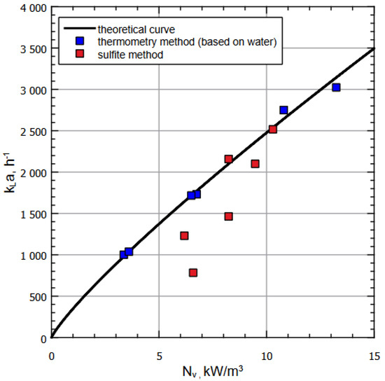
Figure 5.
Dependence of on for various liquids and methods of measuring based on archive data (with working volume of the next order than the experimental setup considered above.
4. Discussion
The experimental and theoretical analyses of one of the key characteristics of fermentation apparatuses, namely the volumetric mass transfer coefficient, provided with various methods, are believed to be the first of their kind conducted for various input parameters of the system (frequency, various types of liquid, including the model one, corresponding in rheology to real cultural liquid of biotechnological productions) for various scales of experimental setups of jet bioreactors. At the same time, the authors would like to draw the readers’ attention to a number of requirements for both the experiments and the conclusions following from the analysis of the data. Thus, special requirements should be imposed on minimizing the spread of ambient temperature (which corresponds to the temperature difference during the analysis according to the thermometric method): the temperature measurement calculation error has the same order of magnitude with the temperature difference during thermometry at low powers or at short measurement times. Among the conclusions obtained, we should especially note that all the studied methods for measurements have their limitations in terms of ranges of applicability. For example, for the thermometric method on the one hand, at low pump powers, the thermal power of heating the liquid is comparable to the error in thermal power due to specific of instruments, which allows evaluate the lower limit of applicability. On the other hand, at high powers, the excessive heating of the liquid will overestimate the specific input power, since only a part of the thermal power corresponds to the power used to dissolve oxygen. In this vein, it would be reasonable to introduce a correction factor that depends on the thermal power as a function that decreases outside the primary range of applicability of the method, which in the future will allow it to be expanded. For thermometric measurements, the heat capacity of the final solution is also important: this must be taken into account when choosing a model liquid. We also note that there are other options for obtaining empirical dependencies of on the specific input power, since even when using the dependence given in the article, variation in multipliers and power exponents is allowed. We especially note that it requires the fitting of the methodological parameters for each specific apparatus. The mechanism of energy distribution in the jet bioreactors requires further research and is one of the prospects for this project’s team.
5. Conclusions
The key characteristic of fermentation apparatuses considered in this manuscript, namely the volumetric mass transfer coefficient, indeed draws researchers’ attention both in terms of their fundamental interest in fluid flow research and measurement techniques in closed mass transfer apparatuses circuits and in terms of industry demands. It should be especially highlighted that the measurement technique is particularly challenging and requires adjustments for various bioreactor designs, while classical approaches do not provide the corresponding measurements by, e.g., the sulfite method due to the large scale of installations in industrial solutions. Thus, a verified method for obtaining data on the volumetric mass transfer coefficient with the determination of the objective horizons of application is required, and exactly this approach was demonstrated for the first time in this work. In the presented study, the experimental hydrodynamic and mass transfer characteristics of the jet fermenter were obtained, and the verification of the thermometric approach for estimating the volumetric mass transfer coefficient based on experimental data and the reference sulfite method was carried out. The intervals of applicability of these methods were analyzed, and the critical values for the operating modes of the experimental installations under consideration, designed in full accordance with jet bioreactors in terms of hydrodynamic characteristics, were determined. This study demonstrates the need for a comprehensive analysis of the system using various methods to determine the values of the volumetric mass transfer coefficient. The presented thermometric method for determining the rate of dissolution of atmospheric oxygen can be used in the microbiological and food industries in the development of new types of fermentation equipment in order to determine the best indicators for mass transfer, as well as to compare various types of apparatus that differ in design and energy input for mixing and aeration, and also to determine the mass-transfer parameters of industrial mass-exchange/fermentation apparatuses of large unit power. The development of the various novel engineering solutions, techniques, and methodology in fermentation are aimed to improve process efficiency, safety, and other process parameters, which are crucial to shaping a wide spectrum of biotechnology products’ quality.
Author Contributions
Conceptualization, I.S. and I.N.; methodology, V.S. and D.C.; software, P.M. and S.V.; formal analysis, S.L. and N.K.; investigation, I.S., V.S., I.N. and S.L.; resources, D.C.; data curation, I.S. and P.M.; writing—original draft preparation, I.S., I.N., P.M., S.L., N.K. and V.S.; writing—review and editing, I.S., I.N., P.M., S.L. and V.S.; visualization, I.S. and P.M.; supervision, S.L. and D.C.; project administration, D.A. and D.C.; funding acquisition, I.S. and D.C. All authors have read and agreed to the published version of the manuscript.
Funding
The research funding from the Ministry of Science and Higher Education of the Russian Federation (Ural Federal University Program of Development within the Priority-2030 Program) is gratefully acknowledged.
Acknowledgments
The authors express their heartfelt gratitude to Professor Evgeny L. Listov for their professional consultation, historical references and friendly support of the study.
Conflicts of Interest
The authors declare no conflict of interest.
Nomenclature
| density of the liquid, | |
| dissolved oxygen concentration in the liquid, (kg/L) | |
| equilibrium dissolved oxygen concentration in the liquid, (kg/L) | |
| heat loss, (J) | |
| total coefficient of heat transfer by radiation and convection, (W/(m | |
| heat exchange surface area, (m) | |
| surface temperature of the apparatus, () | |
| ambient temperature, () | |
| measurement period, (s) | |
| temperature of the liquid, | |
| liquid temperature difference during the measurement, | |
| specific heat capacity of the liquid, | |
| specific input power (thermal), | |
| specific input power (at the pump impeller), , calculated taking into account pump and liquid specific characteristics | |
| volumetric mass transfer coefficient, |
References
- Guseva, E.M.N.; Safarov, R.; Boudrant, J. An approach to modeling, scaling and optimizing the operation of bioreactors based on computational fluid dynamics. Int. J. Softw. Prod. Syst. 2015, 112, 249–255. [Google Scholar]
- Petersen, L.A.; Villadsen, J.; Jørgensen, S.B.; Gernaey, K.V. Mixing and mass transfer in a pilot scale U-loop bioreactor. Biotechnol. Bioeng. 2017, 114, 344–354. [Google Scholar] [CrossRef] [PubMed]
- Prasser, H.M.; Häfeli, R. Signal response of wire-mesh sensors to an idealized bubbly flow. Nucl. Eng. Des. 2018, 336, 3–14. [Google Scholar] [CrossRef]
- Krychowska, A.; Kordas, M.; Konopacki, M.; Grygorcewicz, B.; Musik, D.; Wójcik, K.; Jędrzejczak-Silicka, M.; Rakoczy, R. Mathematical modeling of hydrodynamics in bioreactor by means of CFD-based compartment model. Processes 2020, 8, 1301. [Google Scholar] [CrossRef]
- Yao, Y.; Fringer, O.B.; Criddle, C.S. CFD-accelerated bioreactor optimization: Reducing the hydrodynamic parameter space. Environ. Sci. Water Res. Technol. 2022, 8, 456–464. [Google Scholar] [CrossRef]
- Panunzi, A.; Moroni, M.; Mazzelli, A.; Bravi, M. Industrial Case-Study-Based Computational Fluid Dynamic (CFD) Modeling of Stirred and Aerated Bioreactors. ACS Omega 2022, 7, 25152–25163. [Google Scholar] [CrossRef]
- Ramírez, L.A.; Pérez, E.L.; García Díaz, C.; Camacho Luengas, D.A.; Ratkovich, N.; Reyes, L.H. CFD and Experimental Characterization of a Bioreactor: Analysis via Power Curve, Flow Patterns and kLa. Processes 2020, 8, 878. [Google Scholar] [CrossRef]
- Cappello, V.; Plais, C.; Vial, C.; Augier, F. Scale-up of aerated bioreactors: CFD validation and application to the enzyme production by Trichoderma reesei. Chem. Eng. Sci. 2021, 229, 116033. [Google Scholar] [CrossRef]
- Nizovtseva, I.G.; Starodumov, I.O.; Schelyaev, A.Y.; Aksenov, A.A.; Zhluktov, S.V.; Sazonova, M.L.; Kashinsky, O.N.; Timkin, L.S.; Gasenko, V.G.; Gorelik, R.S.; et al. Simulation of two-phase air–liquid flows in a closed bioreactor loop: Numerical modeling, experiments, and verification. Math. Methods Appl. Sci. 2022, 45, 8216–8229. [Google Scholar] [CrossRef]
- Biessey, P.; Bayer, H.; Theßeling, C.; Hilbrands, E.; Grünewald, M. Prediction of Bubble Sizes in Bubble Columns with Machine Learning Methods. Chem. Ing. Tech. 2021, 93, 1968–1975. [Google Scholar] [CrossRef]
- Cruz, I.A.; Chuenchart, W.; Long, F.; Surendra, K.; Andrade, L.R.S.; Bilal, M.; Liu, H.; Figueiredo, R.T.; Khanal, S.K.; Ferreira, L.F.R. Application of machine learning in anaerobic digestion: Perspectives and challenges. Bioresour. Technol. 2022, 345, 126433. [Google Scholar] [CrossRef] [PubMed]
- Hessenkemper, H.; Starke, S.; Atassi, Y.; Ziegenhein, T.; Lucas, D. Bubble identification from images with machine learning methods. arXiv 2022, arXiv:2202.03107. [Google Scholar]
- Yu, S.I.; Rhee, C.; Cho, K.H.; Shin, S.G. Comparison of different machine learning algorithms to estimate liquid level for bioreactor management. Environ. Eng. Res. 2022, 28, 220037. [Google Scholar] [CrossRef]
- Rathore, A.S.; Kanwar Shekhawat, L.; Loomba, V. Computational Fluid Dynamics for Bioreactor Design. In Bioreactors: Design, Operation and Novel Applications; Wiley Online Library: Hoboken, NJ, USA, 2016; pp. 295–322. [Google Scholar]
- Ansoni, J.L.; Seleghim, P., Jr. Optimal industrial reactor design: Development of a multiobjective optimization method based on a posteriori performance parameters calculated from CFD flow solutions. Adv. Eng. Softw. 2016, 91, 23–35. [Google Scholar] [CrossRef]
- Charles, M. Fermentation scale-up: Problems and possibilities. Trends Biotechnol. 1985, 3, 134–139. [Google Scholar] [CrossRef]
- Gill, N.; Appleton, M.; Baganz, F.; Lye, G. Quantification of power consumption and oxygen transfer characteristics of a stirred miniature bioreactor for predictive fermentation scale-up. Biotechnol. Bioeng. 2008, 100, 1144–1155. [Google Scholar] [CrossRef]
- Petříček, R.; Labík, L.; Moucha, T.; Rejl, F.J.; Valenz, L.; Haidl, J. Volumetric Mass Transfer Coefficient in Fermenters: Scale-up Study in Viscous Liquids. Chem. Eng. Technol. 2017, 40, 878–888. [Google Scholar] [CrossRef]
- Schügerl, K. Comparison of different bioreactor performances. Bioprocess Eng. 1993, 9, 215–223. [Google Scholar] [CrossRef]
- Moser, A. Bioreactor Performance: Process Design Methods. In Bioprocess Technology; Springer: Berlin/Heidelberg, Germany, 1988; pp. 307–405. [Google Scholar]
- Stanbury, P.F.; Whitaker, A.; Hall, S.J. Principles of Fermentation Technology; Elsevier: Amsterdam, The Netherlands, 2013. [Google Scholar]
- Halme, A.; Kiviranta, H.; Kiviranta, M. Study of a single-cell protein fermentation process for computer control. Ifac Proc. Vol. 1977, 10, 407–415. [Google Scholar] [CrossRef]
- Pilarek, M.; Sobieszuk, P.; Wierzchowski, K.; Dąbkowska, K. Impact of operating parameters on values of a volumetric mass transfer coefficient in a single-use bioreactor with wave-induced agitation. Chem. Eng. Res. Des. 2018, 136, 1–10. [Google Scholar] [CrossRef]
- Šulc, R.; Dymák, J. Hydrodynamics and Mass Transfer in a Concentric Internal Jet-Loop Airlift Bioreactor Equipped with a Deflector. Energies 2021, 14, 4329. [Google Scholar] [CrossRef]
- Bun, S.; Wongwailikhit, K.; Chawaloesphonsiya, N.; Lohwacharin, J.; Ham, P.; Painmanakul, P. Development of modified airlift reactor (MALR) for improving oxygen transfer: Optimize design and operation condition using ‘design of experiment’methodology. Environ. Technol. 2020, 41, 2670–2682. [Google Scholar] [CrossRef] [PubMed]
- Hibiki, T.; Goda, H.; Kim, S.; Ishii, M.; Uhle, J. Experimental study on interfacial area transport of a vertical downward bubbly flow. Exp. Fluids 2003, 35, 100–111. [Google Scholar] [CrossRef]
- Kreitmayer, D.; Gopireddy, S.R.; Matsuura, T.; Aki, Y.; Katayama, Y.; Nakano, T.; Eguchi, T.; Kakihara, H.; Nonaka, K.; Profitlich, T.; et al. CFD-Based and Experimental Hydrodynamic Characterization of the Single-Use Bioreactor XcellerexTM XDR-10. Bioengineering 2022, 9, 22. [Google Scholar] [CrossRef] [PubMed]
- Vaidheeswaran, A.; Hibiki, T. Bubble-induced turbulence modeling for vertical bubbly flows. Int. J. Heat Mass Transf. 2017, 115, 741–752. [Google Scholar] [CrossRef]
- Ohba, K.; Yuhara, T.; Matsuyama, H. Simultaneous measurements of bubble and liquid velocities in two-phase bubbly flow using laser Doppler velocimeter. Bull. JSME 1986, 29, 2487–2493. [Google Scholar] [CrossRef]
- Maischberger, T. Optimized process and bioreactor characterization. Chem. Ing. Tech. 2019, 91, 1719–1723. [Google Scholar] [CrossRef]
- Bun, S.; Chawaloesphonsiya, N.; Ham, P.; Wongwailikhit, K.; Chaiwiwatworakul, P.; Painmanakul, P. Experimental and empirical investigation of mass transfer enhancement in multi-scale modified airlift reactors. Multiscale Multidiscip. Model. Exp. Des. 2020, 3, 89–101. [Google Scholar] [CrossRef]
- Richard, H.; Irina, N.; Dmitri, C.; Kalyuzhnaya, M.G. C1-Proteins Prospect for Production of Industrial Proteins and Protein-Based Materials from Methane. In Algal Biorefineries and the Circular Bioeconomy; CRC Press: Boca Raton, FL, USA, 2022; pp. 251–276. [Google Scholar]
- Strong, P.; Kalyuzhnaya, M.; Silverman, J.; Clarke, W. A methanotroph-based biorefinery: Potential scenarios for generating multiple products from a single fermentation. Bioresour. Technol. 2016, 215, 314–323. [Google Scholar] [CrossRef]
- Listov, E.L.; Chernushkin, D.V.; Burov, S.N.; Dibtsov, V.P.; Sorokin, A.G.; Butorova, I.A.; Aksyutin, O.E.; Ishkov, A.G.; Bondarenko, K.N.; Shajkhutdinov, A.Z.; et al. Method for Determining Mass-Exchange Apparatus Efficiency. RUS Patent RU 2702539 C1, 20 February 2019. [Google Scholar]
- Wallis, G. One-Dimensional Two-Phase Flow; McGraw Hill: New York, NY, USA, 1969. [Google Scholar]
- Levich, V. Physicochemical Hydrodynamics; Prentice-Hall: Upper Saddle River, NJ, USA, 2017. [Google Scholar]
- Viestur, U.; Kuznetsov, A.; Savenkov, B. Sistemy Fermentacii; Zinatne: Riga, Latvia, 1986. [Google Scholar]
- Kirillin, V.; Sychev, V.; Sheindlin, A. Technical Thermodynamics; Izdatel Energiia: Moscow, Russia, 1974. [Google Scholar]
- Nazarov, V. Processes and devices of microbiological productions. J. Tech. Res. 2016, 2, 4. [Google Scholar]
- Vinogradova, A.; Anashkina, E. Obshchaya Biotekhnologiya; Perm University Press: Perm Krai, Russia, 2008. [Google Scholar]
- Khabibrahmanov, R.; Muhachev, S. Issledovanie massoobmennyh harakteristik apparatov s perforirovannymi meshalkami sul’fitnym metodom. Vestn. Kazan. Tekhnologicheskogo Univ. 2014, 17, 140–143. [Google Scholar]
- Mironov, M.; Tokareva, M. Metody Rascheta Oborudovaniya Biotekhnologicheskih Proizvodstv; Urals University Press: Chelyabinsk, Russia, 2017. [Google Scholar]


Publisher’s Note: MDPI stays neutral with regard to jurisdictional claims in published maps and institutional affiliations. |
© 2022 by the authors. Licensee MDPI, Basel, Switzerland. This article is an open access article distributed under the terms and conditions of the Creative Commons Attribution (CC BY) license (https://creativecommons.org/licenses/by/4.0/).