Abstract
CFD-DEM modelling of particle-laden turbulent flow is challenging in terms of the required and obtained CFD resolution, heavy DEM computations, and the limitations of the method. Here, we assess the efficiency of a particle-tracking solver in OpenFOAM with RANS-DEM and LES-DEM approaches under the unresolved CFD-DEM framework. Furthermore, we investigate aspects of the unresolved CFD-DEM method with regard to the coupling regime, particle boundary condition and turbulence modelling. Applying one-way and two-way coupling to our RANS-DEM simulations demonstrates that it is sufficient to include one-way coupling when the particle concentration is small (O ~ ). Moreover, our study suggests an approach to estimate the particle boundary condition for cases when data is unavailable. In contrast to what has been previously reported for the adopted case, our RANS-DEM results demonstrate that simple dispersion models considerably underpredict particle dispersion and previously observed reasonable particle dispersion were due to an error in the numerical setup rather than the used dispersion model claiming to include turbulence effects on particle trajectories. LES-DEM may restrict extreme mesh refinement, and, under such scenarios, dynamic LES turbulence models seem to overcome the poor performance of static LES turbulence models. Sub-grade scale effects cannot be neglected when using coarse mesh resolution in LES-DEM and must be recovered with efficient modelling approaches to predict accurate particle dispersion.
1. Introduction
Two-phase systems consisting of a continuum phase (fluid) and a discrete phase (particles) are prevalent in industrial processes, biological phenomena, and nature. The behavior of solid particles in continuous fluid flow is determined by complex physics and depends on the particle and fluid characteristics and flow regime. According to Crowe at al. [1], five key factors contribute to the turbulence modulation induced by particles: (1) Surface effects: particle size normalized by a length scale ; (2) inertial effects: flow Reynolds number Re and particle Reynolds number Rep; (3) response effects: particle response time or Stokes number St; (4) loading effects: particle volume fraction αp; and (5) interaction effects: particle-particle as well as particle-wall. Numerical simulations of such systems can be helpful in providing a detailed insight into the complex physics involved in particle motion. However, modelling of particle motions in turbulent flow is difficult because it involves the modelling of the surrounding flow field and resulting pressure gradients as well as the particle-flow interaction, which involves the local flow around the particle and the forces resulting from the stress applied on the particle by the flow [2].
In computational fluid dynamics (CFD), both phases can be treated as continuum medium, also called the Eulerian–Eulerian method, in which Navier–Stokes (NS) equations are solved for each phase, including the momentum exchange between the phases. The Eulerian–Eulerian method is computationally less expensive but at the cost of losing the discrete nature of particles. On the other hand, a Lagrangian method is adopted for granular systems, also called the Discrete Element Method (DEM), where each particle is tracked using Newton’s second law of motion. With an increase in computational power, advancements in CFD and DEM, and improved solution algorithms over the last decade, the new and more detailed approach combining CFD and DEM for multiphase systems, called the Eulerian–Lagrangian method (CFD-DEM), has become a popular tool to investigate particle-laden flows. In particular, numerical approaches combining the CFD and DEM have proven to be advantageous over many other options in terms of computational efficiency and numerical convenience [3]. In CFD-DEM, the continuum phase (fluid) is resolved using the NS equations, whereas the discrete phase (particles) is tracked by solving Newton’s second law of motion for each particle in the fluid system. The continuum and discrete phase are also coupled with each other using momentum transfer mechanisms. This coupling level depends on the volumetric fraction of solid material αp = Vp/V in the system, where Vp is particle volume, and V is total volume of particles and fluid. A classification map is depicted in Figure 1, which can be used to incorporate the level of coupling in numerical simulations [4]. Furthermore, the approximated CFD solution can be obtained using Reynolds-averaged Navier–Stokes equations (RANS) or Large-Eddy simulation (LES), instead of solving the flow using Direct Numerical Simulation (DNS), which could save significant computational efforts, especially when tracking particles using DEM.
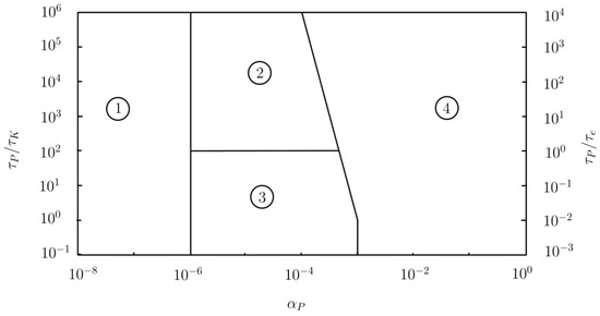
Figure 1.
Classification map [4] showing the level of coupling required for numerical simulations and interaction between particles and turbulence for ① one-way coupling, ② two-way coupling where particles enhance the turbulent production, ③ two-way coupling where particles enhance the turbulence dissipation, ④ four-way coupling.
The CFD-DEM method can be categorized into two approaches: unresolved and resolved CFD-DEM. Unresolved CFD-DEM solves the flow at larger scales using filtering (LES)/averaging (RANS) methods and can only be applied to particles smaller than the CFD cell size. In unresolved CFD-DEM, some empirical equations are used to calculate the fluid forces acting on the particles and the calculated fluid forces are included as additional terms in governing DEM equations. In contrast, resolved CFD-DEM (particle resolved DNS) can be applied to larger particles than the CFD cell size, where extreme fine meshing is used to obtain detailed information on turbulence flow and forces acting on particles are directly obtained by integrating fluid stress over the particle surface. In resolved CFD-DEM, various techniques such as Adaptive mesh refinement (AMR) and Immersed boundary method (IBM) are becoming popular, but are limited to a minimal number of particles [5]. Additionally, the particles can be assumed as point-particles (PP), representing point objects with a certain mass and whereupon DNS can be performed. Unlike resolved CFD-DEM, here the forces acting on the particles are calculated using empirical equations, but the application of PP DNS-DEM to particles larger than Kolmogorov scale is questionable and highly discouraged.
DNS-DEM studies [6,7] are limited to simple flows, a small number of particles, and mainly to the PP approach due to heavy computational requirements. DNS performed on PP in rough-wall pipe with a small Reynold’s number indicates that particle volume fraction (αp) and Stokes number (St) play an important role in turbulent modification [8]. Recently, a two-way coupled DNS study on particle-laden flow highlighted the effects of the particle Stokes number (St) on near-wall turbulence [9]. Resolved CFD-DEM (particle resolved DNS) is only possible if the spacing of the computational grid is small compared to the size of a particle, therefore restricting its application to large particles compared to the smallest scales of the turbulent flows and/or relatively small number of particles [10]. Even for single-phase fluid systems, DNS is not possible for the cases with high Reynolds numbers and complex geometries due to computational limitations.
RANS-DEM is another economical approach where the mean flow fields are obtained, and additional dispersion models incorporate the turbulence effect on the particle’s trajectories. An accurate evaluation of instantaneous velocity fluctuations is required for the realistic evaluation of turbulent diffusion effects for accurate predictions of particle dispersion and deposition on surfaces [11,12]. A number of RANS-DEM studies on simple cases [13,14] indicate that these simple dispersion models cannot accurately obtain the lost fluctuating component due to averaging of NS equations. In contrast, Greifzu et al. [15] showed that the simple dispersion models are indeed able to predict correct particle dispersion even for more complex flow (particle-laden BFS flow). However, we found out that their conclusion was due to an error in the numerical setup (refer to the results and discussion section for details). Therefore, further investigation is necessary to reach a unanimous conclusion about the ability of the simple dispersion models in incorporating the effect of turbulent fluctuations on particle motion.
A sensible and efficient approach would be LES-DEM, which might be a good compromise between accuracy and computational feasibility. However, one also has to be cautious about the sub-grid scales (SGS) fluid fluctuating motion seen by the particles, because in several investigations, the effects of SGS on particle motion were shown to be significant and hence should not be neglected [16,17,18,19], especially when the particle response time is the same order of magnitude as that of the smallest time scale resolved in LES. To recover the dynamic consequences of the SGS in the LES-DEM framework, stochastic models such as an explicit stochastic forcing in the equations of particle motion were suggested [20,21]. Furthermore, the size of LES meshes in unresolved CFD-DEM is restricted by the requirement of particles being significantly smaller than the CFD cell size, unless particles are considered as PP. This restriction prevents finer meshes near the boundaries (y+~1) and can lead to poor performance of the static LES turbulence model, which require very fine boundary meshes. Dynamic LES turbulence models could be adopted to avoid the poor performance of static LES models in cases of low mesh resolutions.
On one hand, commercial software such as Fluent EDEM, STAR-CCM+ and AVL-fire [22,23,24,25,26], in-house CFD programs such as LESOCC [27], and research codes [28,29,30,31] can be applied to CFD-DEM simulations, but the accessibility of these solvers is limited. On the other hand, some open-source CFD codes, such as OpenFOAM [32] have accelerated research in the field. Some coupled CFD-DEM codes [33,34] are also available, which couple OpenFOAM and DEM software such as LAMPS/LIGGGHTS and are not limited to PP.
Particle-laden backward facing step (BFS) flow is popular among researchers in the field due to its simple geometry and ability to produce interesting turbulent features concerning flow separation and re-attachment. A few LES-DEM simulations on particle-laden BFS have been performed [35,36,37,38,39,40], and some have attained a reasonable agreement with the experiment. These LES-DEM studies used extreme fine meshing (y+~1) and were mainly based on the PP approach. The particle-laden BFS flow adopted in our study had previously been numerically simulated by Greifzu et al. [15] in the context of RANS-DEM. The authors concluded that RANS-DEM (and the simple dispersion model therein) predicts the correct fluid and particle velocity profiles, as well as the particle dispersion. Interestingly, we found that their OpenFOAM numerical setup was erroneous as a fluid density of 1000 kg/m3 (water) instead of 1 kg/m3 (air) was used, although in the original experiment the fluid was air, not water. Despite using an incorrect fluid density value, the authors obtained an excellent agreement with the experimental data. However, these results are questionable, as the density of the fluid should have been 1 kg/m3 as in the original experiment—therefore requiring a reinvestigation.
Despite several experimental and numerical studies, fluid-particle systems remain poorly understood due to the complex physics involved, such as turbulent modulation and complex fluid-particle and particle-particle interaction. The CFD-DEM method could provide detailed insights into these multivariable and interdependent phenomena and can be employed for large scale engineering applications. However, due to the huge computational requirements and associated limitations of the CFD-DEM method, finding the trade-off and compromise between the levels of flow resolution obtained (DNS/LES/RANS) and the required computational efforts to predict the correct particle dispersion and trajectories is difficult.
Here, we focus on different aspects of modelling such flows in terms of the computational requirements, the available models, as well as the challenges and limitations. In particular, we perform RANS-DEM and LES-DEM simulations in 3D for particle-laden BFS flow. Special attention is given to the ability of the respective approaches to predict particle dispersion, coupling regime, particle boundary conditions, and turbulence modelling. First, we discuss the theoretical background of the Eulerian–Lagrangian method (CFD-DEM) in detail, focusing on the RANS and LES methods for resolving the fluid flow fields. The following method and numerical setup section highlights the fundamental structural differences in the numerical setup for different approaches adopted in our study. Furthermore, the RANS-DEM and LES-DEM simulation results for the fluid and particle phases are compared, especially in relation to particle dispersion. Additionally, different aspects of the CFD-DEM method with regard to the coupling regime and particle boundary conditions were investigated and their effects on fluid and particle phase results are discussed. Before including particles into the system, single-phase RANS and LES simulations are also performed and its accuracy in predicting mean and turbulent flow statistics with different turbulence models are assessed. Taken together, RANS-DEM requires more sophisticated dispersion models to predict correct particle dispersion, and LES-DEM has limitations in terms of the flow resolution obtained, the computational resources required, and the prerequisites of unresolved CFD-DEM, preventing extreme fine meshing unless the particles are considered as PP.
2. CFD-DEM Approach and the Governing Equations
The unresolved CFD-DEM approach was adopted to investigate the two-phase system containing fluid as a continuum and the particles as discrete mediums. The full NS equations describe the continuum fluid phase for unsteady incompressible flow, which is a slightly modified version of the standard NS equations to incorporate the particle fraction in each computational cell. Newton’s second law of motion describes the discrete particle phase.
where:
α = volume fraction of fluid in each cell; unitless
= fluid velocity field in direction i; m/s
p = fluid pressure; N/m2
= kinematic viscosity of fluid; m2/s
= gravitational acceleration in direction i; m/s2
= density of fluid; kg/m3
= mass of particle k; kg
= number of particles colliding with particle k; unitless
= moment of inertia of particle k; kgm2
= velocity of particle k in direction i; m/s
= angular velocity of particle k in direction i; 1/s
= surface forces acting on particle k (including drag, lift, added-mass, basset history forces etc.: coupled forces); N
= volumetric fluid-particle interaction momentum source in direction i; N/m3
= body forces acting on particle k; (gravity + buoyancy: uncoupled forces)
= ; N
= density of particle; kg/m3
= particle-particle interaction/contact force between particle k and l; N
= particle-particle interaction moment between particle k and l; Nm
x and t are space and time with units m and s, respectively.
= particle-particle interaction moment between particle k and l; Nm
x and t are space and time with units m and s, respectively.
OpenFOAM considers the particles as point-particles (PP), meaning that they are represented as point objects having a certain mass. This assumption automatically neglects the torque acting on the particles, meaning that OpenFOAM does not consider Equation (4) in calculating the trajectories of the particles.
In the above equations, the momentum transfer term consists of several forces coupled between the continuum phase and discrete phase, such as drag force, lift force, pressure gradient force, basset history force, added-mass force, etc. In the references, it has been established that the major contribution in the momentum transfer term originates from the drag force [41], and lift force is more relevant for light particles than heavy particles [10]. The particles considered in the present study are dense copper particles. Therefore, the lift force seems to be insignificant for our case. However, we have also included the pressure gradient force in addition to the drag force in our numerical setup. Ultimately, the coupled forces term reduces to:
From the equations above, one can see that to calculate forces acting on particles (thus to calculate their trajectories), information is needed on the fluid velocity at the location of particle (). We obtain this information from the fluid phase solution (CFD). The solution of fluid phase can be categorized into three types, namely Direct Numerical Simulation (DNS), Large-Eddy Simulation (LES), and Reynolds-averaged Navier–Stokes equations (RANS), depending on the level of flow resolution needed and the computational resources available.
2.1. Direct Numerical Simulation (DNS)
DNS solves the full NS equations numerically, thus resolving everything from the largest scale to the smallest dissipative eddies present in the system. In DNS under consideration of the point-particles (PP) approach, the velocity of the fluid at the particle location can be obtained directly from the DNS solution.
Since turbulent flows possess a varying range of time and length scales, the exact solution (DNS), even for the simplest turbulent flows, requires enormous computational resources and extreme fine meshing. Initial estimation of the computational resources required for DNS can be made based on Kolmogorov scales (smallest time, length and velocity scales) in the system. In our case, the Kolmogorov length scale is about 170 µm, meaning the mesh resolution should be smaller than 170 µm for DNS. It has been demonstrated that the restrictions that DNS needs for simple channel flow in terms of grid point and time steps [42], thus require huge computational resources even for simple channel flow. Computational resources requirement by DNS in the sense of both processor speed and memory size for storing intermediate results is vast and increases exponentially with the Reynolds number of the flow. In order to obtain the maximum possible information about the flow fields with an affordable computational cost, the full NS equations are approximated with some averaging/filtering approaches. The resulting averaged/filtered NS equations have almost the same form as the original NS equations with additional terms, which can be calculated based on eddy viscosity.
2.2. Large-Eddy Simulation (LES)
LES aims to resolve large-scale turbulence while small-scale turbulence is modelled using the filtering operation. Compared to DNS, where nearly all the computational effort is used to resolve the smallest dissipative eddies, LES resolves only up to the inertial subrange, not all the way to the dissipative scales. This can save significant computational effort, yet preserves enough information of the fluid flow. LES converges to DNS when finer meshing and smaller time steps are used.
The common idea behind LES is to decompose the instantaneous flow field into resolved (or filtered) component and residual (or sub-grid scale; SGS) component by a filtering operation, as follows:
where, is the filter function that depends on mesh discretization. The filtering operation results in extra terms, called residual stresses () in the original NS equations. Calculation of residual stresses is based on the Boussinesq hypothesis of eddy viscosity (turbulence viscosity ), which is being modelled. Various models are available for this purpose, such as Smagorinsky, one-equation model (kEqn), dynamic Smagorinsky, dynamicKEqn, Spallart–Allmaras, and many others. We found that the dynamicKEqn turbulence model was able to predict correct flow fields in terms of mean and fluctuating components with reasonable accuracy, whereas static turbulence models were performing poorly with provided mesh resolution.
In cases where the particle response time (Stokes number) is large compared to the smallest time scale resolved in LES, the fluid velocity of the sub-grid scales does not significantly influence the particle’s motion [10,43,44]. Considering this, one does not need an extra dispersion model to incorporate the effect of turbulence in the particle’s motion; thus, the LES solution can be directly equated to the fluid velocity at the location of the particle.
2.3. Reynolds-Averaged Navier–Stokes Equations (RANS)
RANS resolve only the mean flow statistics; thus, RANS solution for fluid flow fields cannot be directly equated with the fluid velocity at the location of the particle. In RANS, the instantaneous flow field decomposes into a time average component and a fluctuating component :
The averaging operation results in some new terms, called Reynolds stresses, to appear in the original NS equations, which are also modelled based on eddy viscosity. The terms , although named as Reynolds stresses, have a unit of stress only when multiplied by the fluid density . Similar to LES, eddy viscosity can be calculated based on several models such as k-ε, k-ω, k-ω SST and many others. We used the k-ω SST model to close the Reynolds-averaged NS equations of our RANS and RANS-DEM simulations, as it was the best performing.
In RANS, the effect of fluctuating components (turbulence) on particles is incorporated using some dispersion models [45]. The resulting fluid velocity at the location of a particle () can be equated to the sum of the RANS (mean) velocity field and the modelled fluctuations.
All three approaches (DNS, LES, and RANS) for calculating the fluid velocity at the location of particles have their limitations in terms of accuracy and computational cost and can be adopted as per the details required and computational resources available. Figure 2 shows the extent of modelling certain types of turbulent models [46], where DNS resolves everything from the largest to the smallest dissipative eddies present in the system. LES resolves up to energy-containing eddies while dissipative eddies are modelled. RANS resolves only the mean flow statistics, and the fluctuating components are modelled. More information on the implementation of the turbulence models used in our RANS-DEM and LES-DEM and the dispersion models can be found on the OpenFOAM webpage [32]. We have used RANS-DEM and LES-DEM approaches to solve particle-laden BFS flow and investigated the case by comparing the fluid and particle-phase results with the experimental data and literature.
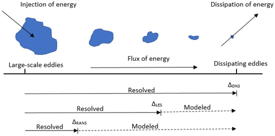
Figure 2.
Extent of modelling for certain types of turbulent flows [46].
2.4. Particle Dispersion Modelling
The approximated NS equations provide mean (RANS)/filtered (LES) flow statistics and information about turbulent fluctuations are lost due to simplifications of original NS equations. The fluid-particle interaction forces () such as pressure gradient force, added mass force, drag force and history force, contain unfiltered components and are required to be estimated to close certain terms in particle equations of motion. In LES-DEM, the sub-grid scales only have a small effect on the particle’s trajectories, especially when the particle response time is large compared to the typical time scales of the turbulent flow and the smallest time scale resolved in LES. However, the sub-grid scales can be significant in many physical processes such as in turbophoresis [17]. On the other hand, the effect of turbulent fluctuations must be included in RANS-DEM to predict realistic particle trajectory. There are mainly two types of modelling approaches to account for missing turbulent fluctuations: either by adding stochastic noise forcing to the NS equations [47] or by adding an additional velocity to the particle equation of motion [48]. The stochastic models, which aim to recover the lost turbulence effects on a particle’s trajectories, can be formulated based on (a) transport equations of the turbulent kinetic energy (Discrete Random Walk; DRW, or Eddy Interaction Model; EIM) or (b) generalized Langevin equation (Continuous Random Walk; CRW). We have considered the DRW/EIM stochastic model in our numerical simulation. Here, particles are assumed to be trapped by an eddy during its lifetime, resulting in the mean flow fields seen by the particles being those of the fluid and the fluctuating components, which are randomly distributed following Gaussian distribution, whose root mean square values are equal and deduced from the turbulent kinetic energy.
In OpenFOAM, two dispersion models are available to model the turbulent fluctuations , namely StochasticDispersionRAS and GradientDispersionRAS models, which are basically DRW/EIM type of stochastic dispersion models. These dispersion models use the turbulent kinetic energy (TKE; ) provided by the RANS solution to model the turbulence fluctuations such that,
where is a random factor that reproduces a probability density function with Gaussian distribution with an expected value µ = 0 and standard deviation σ = . is a unit vector that points either in a random direction (in StochasticDispersionRAS) or in −k (in GradientDispersionRAS).
2.5. Coupling between Continuum and Discrete Phases
As shown in Figure 1, the continuum and discrete phases interact with each other and are required to be coupled. Several studies have emphasized on one-way and two-way coupling [49,50,51,52] for dilute particle-laden flows and fluid-structure interaction. Depending on the coupling regime, specific terms vanish in the respective governing equations. The coupling regime required for numerical simulations can be made using the volumetric particle concentration (αp).
- One-way coupling (fluid → particle): when the volumetric concentration of particles is small (αp < 0.0001%), the fluid flow fields affect the particle motion, but particles have a negligible effect on fluid flow fields. This results in only specific terms being considered in the governing CFD-DEM equations as follows:
- Two-way coupling (fluid ←→ particle): when the volumetric concentration of particles increases (0.1% < αp < 0.0001%), both fluid and particles affect each other’s motion. Two-way coupling can be further categorized into two categories, one in which particles enhance the turbulence dissipation and a second in which particles enhance turbulence production, which depends on the ratio of particle reaction time () to the Kolmogorov time scale () and to the turnover time of large eddies (), respectively, where is the density of particle, is the diameter of particle, is the density of fluid, υ is the kinematic viscosity of fluid, is turbulence dissipation rate, is turbulence length scale, and u is the fluid velocity. Two-way coupling results in the following CFD-DEM equations:
- Four-way coupling (fluid ←→ particle, particle ←→ particle): When the volumetric concentration of the particles further increases (αp > 0.1%), the interaction among particles becomes significant. In this regime, fluid and particle affect each other’s motion; additionally, the particle collision term needs to be included in the governing equations:
3. Method and Numerical Setup
The original experiment [53] includes a blower and particle feeders, where the blower injects fluid (air), and the particle feeders feed the particles into the system at a specific mass flow rate. This arrangement provides uniform fluid velocity and particle loading at the inlet of the development section, which has a length of 5.2 m, ensuring that the turbulent flow is fully developed at the inlet of the test section (backward facing step; BFS) and gives the particles enough time/length to become uniformly mixed with the fluid flow and attain equilibrium with the fluid phase before it reaches the inlet of BFS. The fully developed turbulent flow has a centerline velocity of 10.5 m/s, and the Reynolds numbers based on it are 13,800 and 18,400 at the channel section (based on channel half-height h) and at the step (based on step height H), respectively. The geometry of the test section, fluid (air) and particle-phase description in the experiment and their corresponding adoption for numerical simulations are shown in Table 1.

Table 1.
Geometry, fluid, and particle phase characteristics in the original experiment [53] and their corresponding setting for the numerical setup.
The geometry considered (test section; BFS) for numerical simulation can be seen in Figure 3. Due to computational limitations, the development channel before the inlet of BFS is not considered in the geometry. To achieve a fully developed turbulent flow at the inlet of BFS without providing a development channel, mapped boundary conditions are applied, in which flow fields are mapped from 400 mm downstream of the inlet of BFS, resulting in a fully developed fluid velocity profile at the inlet of BFS with a centerline velocity (U0) of 10.5 m/s and average velocity (Uavg) of 9.39 m/s. Regarding the particle boundary condition in OpenFOAM, in addition to the mass flow rate (mass flux) of particles, one also needs to provide a particle injection velocity. In the original experiment, particle velocity was not measured at the inlet of the BFS; thus, no data is available for specifying boundary conditions at the model inlet concerning particle injection velocity. We have tested several boundary conditions for the particle injection velocity. Assuming that all the particles have attained a constant velocity (injection velocity) as they reach the inlet of the BFS, two extreme bounds of particle injection velocity are tested, where the particles are injected with (10.5, 0, 0) m/s (upper bound) and (0, 0, 0) m/s (lower bound) of injection velocity. Furthermore, we assume that the particles have attained a velocity that follows the mean fluid velocity profile at the inlet, which is also tested (i.e., particles injected at the center will have an injection velocity similar to the centerline velocity of the fluid, whereas particles injected near to the walls will have almost zero injection velocity due to the no-slip boundary condition for the fluid phase). The options mentioned above for obtaining the best approximation of particle boundary conditions are tested against both the approaches adopted in our study to simulate particle-laden BFS flow.
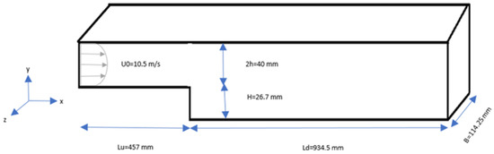
Figure 3.
The geometry considered for numerical simulation.
RANS-DEM and LES-DEM simulations are performed in 3D. In the first step, RANS-DEM simulations were performed for a 10% mass loading of ~70 µm copper particles for one-way and two-way coupling. Although the volumetric particle fraction (O ~ ) lies in the range of two-way coupling, we have also considered one-way coupling in addition to two-way coupling under RANS-DEM to facilitate the comparison between them. Interestingly, our RANS-DEM results almost overlap for one-way coupling and two-way coupling, indicating that it should be enough to include one-way coupling, even when the particle concentration is slightly greater than the threshold suggested by Elghobashi [4]. However, we decided to only use two-way coupling for our LES-DEM simulations for 10% mass loading of ~70 µm copper particles due to the fact that the particle volume fraction lies in range of two-way coupling and the CPU time for the case was roughly the same for one-way and two-way coupled RANS-DEM simulations (~10 min more). RANS-DEM and LES-DEM have basic structural differences in their numerical setup as they both require different input parameters, depending on the models used to close the averaged/filtered NS equations. We have used the k-ω SST (kOmegaSST) and dynamicKEqn turbulence models in the case of RANS-DEM and LES-DEM, respectively. We have ensured that the single-phase results match the experimental data before the particles are included in it. In our single-phase LES simulations, we have tested the predictive capability of static turbulence model (kEqn) as well. Once the correctness of the single-phase results has been verified, the cases were modified to incorporate particles and solved using the DPMFoam solver. Although DPMFoam is based on the discrete parcel method (DPM), we have considered only one particle in each parcel, therefore it is equivalent to the discrete element method (DEM). More details about the RANS-DEM and LES-DEM case setup can be found in Table 2.
Table 2.
RANS-DEM and LES-DEM settings.
As mentioned in the introduction, unresolved CFD-DEM requires the CFD mesh to be much larger than the particle size. This is assured as the smallest CFD mesh cell size is 0.2 mm and 0.15 mm in our RANS and LES setup, respectively, which is much greater than the particle size (~70 µm), thus considering them as point-particles (PP) is justified. To resolve the interesting flow features developing near walls, mesh grading is performed, providing us with the flexibility to provide larger cells away from the wall, which saves some additional computational efforts. Mesh is also refined in streamwise direction near the step, whereas uniform mesh is used in spanwise direction. Before we finalize our final mesh, the mesh is refined in a stepwise manner until we obtain almost the same results for fluid and particle velocity profiles between consecutive refinements (grid independence). The selection y+ as 3 instead of 1 in our LES-DEM simulations allowed us to keep the particle size significantly smaller than the CFD cell (PP approach), and extreme fine meshing is avoided due to computational limitations and the resources available. In the review published on LES simulations [54], it has been reported that dynamic LES models are expected to perform better than static models. Our investigation on LES turbulence models also showed that static LES turbulence models such as Smagorinsky or kEqn models cannot predict correct fluid velocity flow fields with the provided mesh resolution (y+~3). Therefore, we used the dynamicKEqn model in our LES-DEM simulations, which seems to overcome the poor performance of static turbulence models when using relatively coarse mesh resolution. However, standard DPMFoam solver does not come with dynamic turbulence models in OpenFOAM-v1912 (the solver used in our RANS-DEM and LES-DEM study), and we needed to compile the dynamicKEqn model as a separate library for two-phase systems and included it in our LES-DEM simulations.
OpenFOAM solvers, namely pimpleFoam and DPMFoam, are used for single and two-phase simulations, respectively, in OpenFOAM-v1912. Both pimpleFoam and DPMFoam use the pimple algorithm to couple velocity and pressure fields. Backward and least Squares schemes are used for time and gradient discretization, respectively. All the divergence terms are discretized using Gauss linear method. The resulting discretized equations were solved using algebraic multigrid (AMG) and algorithms based on a point-implicit linear equation solver (Gauss–Seidel). DEM data (particle position, velocity, etc.) are mapped onto CFD mesh, and particle volume fraction in each computational cell is calculated. The interaction forces are locally averaged in each cell and incorporated in NS equations and the calculated flow data are communicated back to the DEM side. All the simulations were performed in parallel on 56 processors in the Linux cluster of Leibniz Supercomputing Centre (LRZ). The total CPU computational time corresponding to different simulations can be found in Table 3.
Table 3.
Total CPU computational time.
Fluid and particle velocity profiles at the measurement locations are compared with the experimental data. Fluid flow fields can be directly extracted and plotted at the measurement locations from the OpenFOAM results. Time averaging on particles cannot be performed as done for the continuum phase (air) due to the discrete nature of the particles. The particles are evaluated in a slice around the measurement locations with a thickness of 0.15H and the center lies precisely at the measurement locations for every 0.1 s interval from the start to the end of the simulation. The slice thickness of 0.15H is adopted as the same slice thickness was considered for sampling the particles in the previous study [15]. The particle data collected for all the selected time intervals are combined, and averaging is performed in each slice on the particles with the same location (only the y-component). The resulting average particle velocity profiles are then compared with the experimental data.
4. Results and Discussion
The results shown below are arranged in such a way that they indicate the workflow adopted to investigate and solve the particle-laden BFS flow in OpenFOAM. The normalized mean and fluctuating fluid velocity profiles are compared with the experimental data at their respective measurement locations (x/H = 2, 5, 7, 9, 14). Normalized average particle velocity profiles are compared with observed data in the experiment at their respective measurement locations (x/H = 2, 5, 7, 9, 12) to assess the particle-phase results. We have somewhat amplified the normalized velocity fields in order to highlight the deviations.
4.1. Single-Phase RANS and LES
To obtain correct results for discrete phase (particles), one must have acceptable results for the continuum phase (air) with reasonable accuracy. Therefore, we first performed the single-phase RANS and LES simulations using the pimpleFoam solver, which is able to predict fluid velocity profiles with acceptable precision. For RANS and LES results, the methods and formulae used to calculate the fluctuating components () are different. Regarding the RANS models, for everything above mean flow fields, the fluctuating component is calculated (with the assumption of isotropic turbulence holds true) directly from the modelled turbulent kinetic energy (TKE; ) using Equation (22), which is the modelled part of the fluctuating component.
In LES simulations, we aim to resolve 80–90% TKE, and the calculated represents the resolved fluctuating component. is calculated by subtracting the mean flow field from the instantaneous flow fields, as shown below:
where, is the instantaneous velocity, is the time-averaged velocity, and N is the total number of time steps.
Figure 4 compares simulated streamwise air mean and fluctuating velocity profiles under RANS (with kOmegaSST turbulence model) and LES (with kEqn and dynamicKEqn turbulence models) frameworks with the experiment data. It is evident from the streamwise air mean velocity profile plots (Figure 4a) that both RANS and LES (with dynamicKEqn turbulence model) predict the correct mean flow and are able to predict the re-attachment point (x/H ~ 7) quite accurately as observed in the original experiment (x/H ~ 7.4). On the other hand, Figure 4b shows that the streamwise air fluctuating components () from RANS are somewhat underpredicted, which is not surprising as they represent only the modelled part of the turbulent fluctuations. LES (with dynamicKEqn turbulence model) is able to resolve the turbulent fluctuations more accurately and realistically than RANS. LES simulation with static turbulence model (kEqn) performs very poorly with provided LES mesh resolution (y+ ~ 3). The static LES turbulence model is not only unable to predict flow separation but also overpredicts the mean flow and turbulent fluctuating velocities by a huge margin. In LES, the calculated mean and fluctuating velocities represent the statistical fields, which is a function of time over which the averaging is performed (in our case: 3 s). A more accurate and realistic approximation of flow statistics would be obtained if performed over a longer duration. In Figure 5, the simulated velocity fields are shown under (a) RANS and (b) LES (using dynamicKEqn turbulence model) frameworks, representing the level of resolution obtained under these approaches. RANS flow fields are very smooth as they represent mean values, while eddy generation and decay can be seen in LES flow fields. It must be emphasized that with the mesh resolution used in our LES simulations (y+ ~ 3), static LES turbulence models were unable to predict correct fluid velocity profiles, whereas the dynamic LES turbulence model resulted in a relatively real estimation of mean and fluctuating fluid velocity with the used relatively coarser mesh, as shown in our fluid velocity plots.
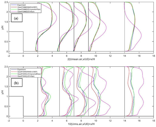
Figure 4.
Comparisons of experimental and OpenFOAM simulated streamwise air (a) mean and (b) fluctuating velocity profiles at the measurement locations under RANS and LES frameworks.
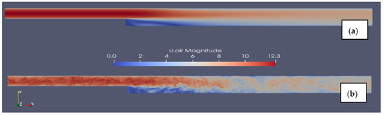
Figure 5.
OpenFOAM simulated velocity fields (magnitude) under (a) RANS (kOmegaSST) and (b) LES (dynamicKEqn) frameworks.
In our next RANS-DEM and LES-DEM sections, we mainly focused on the simulation’s accuracy in predicting particle dispersion on the influence of the carrier fluid (air) flow turbulence. However, even the presence of the particles can modify the turbulence, as discussed in the introduction. The potential modification in air turbulence due to the presence of particles is not explicitly discussed in this study. Additionally, the turbulence models employed do not consider the presence of particles as they are developed for single-phase fluid flow and some works have noticed the potential failure of employed turbulence models in specific flow scenarios [55]. However, new mathematical turbulence models considering the particle’s presence are yet to be developed and do not come under the scope of this study.
4.2. RANS-DEM
We have investigated the effect of one-way and two-way coupling on the continuum and discrete phase results and found almost no difference between the results of either coupling regime. The mass flow rate of 10% and the corresponding volumetric fraction of particles is in order of ~, which is indeed in the range of the two-way coupling threshold suggested by Elghobashi [4]. Interestingly our one-way and two-way coupling results for fluid phase (Figure 6) and particle phase (Figure 7 and Figure 8; red circles) almost overlap each other, suggesting that one-way coupling might also be adopted when particle volumetric fraction is slightly greater (O ~ ) than the threshold for one-way coupling. As demonstrated by our fluid and particle phase results, one-way coupling seems to be sufficient even for particle concentration in O ~ , which is slightly greater than the standard threshold for one-way coupling.
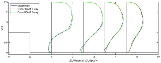
Figure 6.
Comparisons of experimental and OpenFOAM simulated (RANS-DEM) streamwise air mean velocity profiles at the measurement locations for one-way and two-way coupling for the case corresponding to a particle injection velocity of 10.5 m/s.
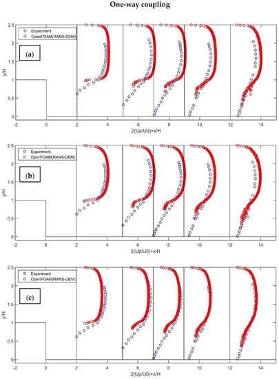
Figure 7.
Comparisons of experimental and OpenFOAM simulated average streamwise particle velocity profiles at the measurement locations for one-way coupling and 10% mass loading of copper particles under RANS-DEM framework. (a) Particle injection velocity as (10.5, 0, 0) m/s, (b) particle injection velocity same as that of the fluid velocity profile at inlet, (c) particle injection velocity as (0, 0, 0) m/s.
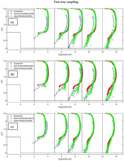
Figure 8.
Comparisons of experimental and OpenFOAM simulated average streamwise particle velocity profiles at the measurement locations for two-way coupling and 10% mass loading of copper particles under RANS-DEM and LES-DEM frameworks. (a) Particle injection velocity as (10.5, 0, 0) m/s, (b) a particle injection velocity same as that of the fluid velocity profile at the inlet, (c) particle injection velocity as (0, 0, 0) m/s.
Figure 9 also shows that when using RANS-DEM, the fluid mean velocity profiles agree very well with the experimental data, as in the single-phase results. For brevity, we show here streamwise air mean velocity profiles (Figure 9) only for two-way coupling corresponding to different particle boundary conditions (injection velocity), as they are very similar to RANS-DEM results for one-way coupling and single-phase RANS results. Figure 9 shows that the air-phase results are independent of particle injection velocities due to small particle concentration. Under the RANS-DEM framework, turbulent fluctuations are significantly underpredicted, which can be seen in single-phase plots, and this underprediction of turbulent fluctuation also reflects in particle velocity plots (Figure 7 and Figure 8; red circles), where particles move roughly like a patch and do not disperse below the step (y/H < 1) even after flow re-attachment (x/H ~ 7). This underprediction of particle dispersion behind the step can also be seen in Figure 10a, which shows the particle spread behind the step at t = 1 s.
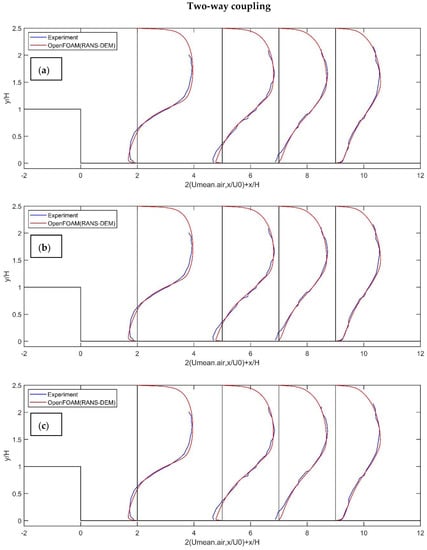
Figure 9.
Comparisons of experimental and OpenFOAM simulated streamwise air mean velocity profiles at the measurement locations for two-way coupling and 10% mass loading of copper particles under RANS-DEM framework. (a) Particle injection velocity as (10.5, 0, 0) m/s, (b) particle injection velocity same as that of the fluid velocity profile at the inlet, (c) particle injection velocity as (0, 0, 0) m/s.
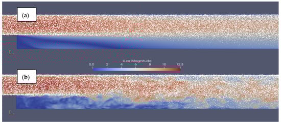
Figure 10.
Screenshot showing particle dispersion behind the step at 1 s under (a) RANS-DEM and (b) LES-DEM frameworks.
One of the main questions that we tried to answer is: how effectively can RANS-DEM, with simple dispersion models, predict particle dispersion in turbulent flows? In other words, its effectiveness in obtaining instantaneous flow fields so that the turbulence effect on the particle’s motion can be modelled accurately. For this purpose, two simple dispersion models are available in OpenFOAM, namely, GradientDispersionRAS and StochasticDispersionRAS, based on Equation (18). An initial investigation reveals that the StochasticDispersionRAS dispersion model gives slightly better results in relation to particle dispersion and was also adopted by Greifzu et al. [15] in their RANS-DEM numerical simulations. Therefore, we decided to use the StochasticDispersionRAS model in our RANS-DEM simulations. Figure 7 shows the normalized streamwise average particle velocity profiles corresponding to one-way coupling for different particle boundary conditions (injection velocity). The results demonstrate that particle-phase results are also very similar for one-way (Figure 7) and two-way coupling (Figure 8), but different particle injection velocities have a notable effect on particle-phase results, unlike air-phase results. When particles are injected with (10.5, 0, 0) m/s of injection velocity from the inlet of BFS (Figure 7a), the particle velocities at all the measurement locations are overpredicted, and their dispersion (spread in the y-direction) is underpredicted. When particles are injected with the velocity that follows the fluid velocity profile at the inlet (Figure 7b), the results improved slightly but were still far from the experimental data, in which the particles moved roughly like a patch, and a minimal number of particles were dispersed below the step (y/H < 1). When particles are injected with (0, 0, 0) m/s of injection velocity (Figure 7c), the particle velocity profiles provide a better match with the experimental data, but the dispersion of the particles is still considerably underpredicted, similar to other RANS-DEM cases. It can also be seen from Figure 8 that a very similar particle dispersion behavior is observed, even for two-way coupling under the RANS-DEM framework. In the RANS-DEM framework, all the cases with different boundary conditions for the particle-phase and under the considered coupling regime underpredict the particle dispersion by a considerable margin and a minimal number of particles are found below the step (y/H < 1) even after the flow re-attachment point (x/H ~ 7). On the other hand, experimental data shows that particles disperse across the extended channel section until they reach the re-attachment point (x/H ~ 7), and, after this, the particle concentration below and above the step becomes almost uniform. Our analysis shows that the simple dispersion models (DRW) are ineffective in incorporating turbulence effects on the trajectory of particles.
In comparison to the RANS-DEM results of Greifzu et al. [15], our fluid flow results are in good agreement with them and with the experimental data as well, but the particle-phase results are entirely different. Their results showed that the RANS-DEM (and simple dispersion model therein) can predict the correct particle dispersion and their velocity profiles. Interestingly, we found that they were using a fluid density of 1000 kg/m3 (water) instead of 1 kg/m3 (air) in their OpenFOAM numerical setup, even though the fluid used in the experiment was air, not water. Using a density of 1000 kg/m3 results in a higher body (buoyant force) and coupled forces (drag and pressure gradient force) acting on the particles, which would disperse the particles in the domain even before the re-attachment point, as observed in the particle velocity plots of Greifzu et al. [15]. It is demonstrated that particles will be dispersed into the recirculation region only when their large-eddy Stokes numbers are less than one [56]. The large-eddy Stokes numbers for fluid as air (density = 1 kg/m3) and as water (density = 1000 kg/m3) are found to be 6.9 and 0.053, respectively. Obviously, when the fluid density is that of water, the Stokes number is significantly smaller than one, so the particles will also be dispersed into the recirculation region (as they behave similar to tracers). Fluid flow results remain almost the same even if the density of water is used instead of air because the momentum transferred from the particle phase to the fluid phase remains of the same order of magnitude. This can be explained as small particle concentrations result only in a few numbers of particles in each computational cell and are simply not numerous enough to modify the fluid flow fields. So, even by considering two-way coupling and a density of fluid as that of water does not modify the fluid flow fields. This explanation also indicates that the previous observation regarding the ability of the simple dispersion model (DRW) in accurately incorporating turbulence effects on particle’s trajectory is not true and supports our observation about simple dispersion models.
The dispersion models available in OpenFOAM are essentially discrete random walk (DRW) type models and are calculated using the modelled turbulent kinetic energy (TKE). These models are simple models based on rough assumptions, e.g., that the turbulence is isotropic in the whole domain, which leads to the inappropriate modelling of turbulence seen by particles. However, the turbulence is very anisotropic in the boundary layers, and this anisotropic behavior is even more significant for wall-bounded flows with complex geometries such as BFS flow. The shortcomings of the discrete random walk (DRW) type of dispersion models can be avoided by better treatment of boundary layer effects. For this purpose, an option could be the Continuous Random Walk (CRW) method to be included in OpenFOAM, which offers a more physically sound way of modelling particle dispersion [57]. The anisotropic behavior of turbulent flow is better modelled using the CRW method, recently presented by Mofakham [13]. An alternative stochastic approach to describe the particle dispersion due to turbulence could be a straightforward generalization of the stochastic approach introduced by Pope [58], which was originally developed to describe single-phase flow. This approach is extended to describe the two-phase system by Peirano et al. [59]. Xiang [14] used this stochastic model in their numerical simulation in OpenFOAM and reported that it performs better than the already implemented dispersion models (DRW models) in OpenFOAM. Although even with their implemented stochastic model, the simulated particle dispersion was far from the reference data. There are also the Reynolds stress transport models (RSTM) that directly evaluate the components of Reynolds stresses and account for the anisotropy of turbulent fluctuations [60,61,62]. However, knowledge of instantaneous fluctuations is required for specific problems, such as the one involving particle dispersion and deposition. It was recently shown that a RANS approach in conjunction with RSTM and DRW does not improve the results in terms of particle dispersion, and that more sophisticated dispersion models such as CRW must be used [13].
In the original experiment, the particles traversed a sufficient distance (a development channel length of 5.2 m) before they reached the inlet of BFS. This assured that the particles had attained equilibrium with the fluid phase before the inlet of BFS, as they had enough time (at least three particle response time, in the worst case) to come to equilibrium with the fluid phase [53]. As at the inlet of BFS, the particle velocity profile was not measured and/or available in the literature, and we do not know the exact particle velocity when they reach the inlet of BFS. It is quite difficult to approximate the real particle velocities at the inlet of BFS without this development channel. Our results demonstrate that the straightforward assumption that all the particles have attained mean flow velocity seems unreasonable. The best approximation of particle injection velocity was found to correspond to an injection velocity of (0, 0, 0) m/s. This might be due to the fact that the particles may obtain real physical velocity depending upon the particle reaction time and fluid flow around it. The additional injection velocity, which one needs to provide along with the mass flux of the particles, does not seem to be necessary as we specify mass flux of particles (e.g., kg/s) that is injected from the inlet of the BFS. Once the particles are in the domain, they attain velocities depending upon the flow around them and the particle response time (Stokes number). However, this approach may vary in individual cases, and the results might look different when the inlet channel (before BFS) length is increased. It also depends on the different algorithms that different software use for particle generation and insertion. The best practice guidelines for CFD should still be the extension of the inlet channel length and allowing particles to develop real physical velocity, but this might be extra computational overhead for CFD-DEM simulations.
4.3. LES-DEM
We decided to perform LES-DEM simulations to investigate the case in more detail; fluid flow fields are calculated using the LES approach, then particle trajectories are calculated based on resolved LES fluid flow fields without considering additional models to include the effects of SGS on the motion of the particle. LES-DEM simulated fluid-flow fields agree well with the experimental data, such as single-phase LES simulations. LES-DEM simulated fluid velocity profiles are not shown here for the sake of brevity. The LES-predicted turbulent fluctuation was a significant improvement over the RANS approach (see Figure 4b), and this is also reflected in particle dispersion, as seen in Figure 8 (green circles) and Figure 10b.
Figure 8 shows normalized streamwise average particle velocity profiles for 10% mass loading of ~70 µm copper particles for two-way coupling corresponding to the different options concerning the particle injection velocities under RANS-DEM (red circles) and LES-DEM (green circles) frameworks. Compared to the RANS-DEM results, particle dispersion and velocity profiles have been improved considerably due to the ability of LES to resolve flow fields in greater detail and improved predictions in view of the improved representation of the flow field seen by the particles. Moreover, when the particles are injected with an injection velocity of (10.5, 0, 0) m/s from the inlet (Figure 8a), the particle velocities at all measurement locations are slightly overpredicted. When particles are injected with an injection velocity that follows the fluid velocity profile at the inlet (Figure 8b), the particle velocity profiles seem to be slightly overpredicted compared to those observed in the experiment. When particles are injected with an injection velocity of (0, 0, 0) m/s from the inlet of BFS (Figure 8c), the particle velocity profiles give a reasonably good match with the experimental data at all the measurement locations. In all the three LES-DEM cases, a very small number of particles is found in the recirculation region, but after the re-attachment point (x/H ~ 7), enough particle dispersion is predicted as observed in the original experiment. Compared to the original experiment, our LES-DEM still underpredicts the particles’ dispersion, especially in the recirculation region. Taking both the correctness of predicting particle velocity and their dispersion into account, we found that the best results were obtained when particles are injected with (0, 0, 0) m/s of injection velocity, and the probable reason of it being the best option to approximate the particle boundary condition without extending the inlet channel is already explained in our RANS-DEM section.
It can be clearly seen that the overall particle-phase results have improved considerably with the LES-DEM approach. The particle-phase results, especially its dispersion, under the LES-DEM framework can be further improved with increased mesh resolution (y+~1) and/or with the inclusion of missing SGS in the equation of particle motion. However, one must always bear in mind that extreme fine meshing can cause stability problems, as CFD cells cannot be smaller than particle diameter under the unresolved CFD-DEM framework, and can thus only be applied under consideration of point-particles (PP). Additionally, further mesh refinement would require much more computational resources. A recent study indicates that the use of stochastic dispersion models is necessary even in the LES-DEM framework, especially for the fine particles, where the corresponding particle relaxation time is of the same order as the smallest fluid flow time scale [63]. Our LES-DEM results also indicate that the effect of SGS cannot be neglected and has a significant effect on particle trajectories, especially for the particles with a small Stokes number, which was also suggested by Ref. [10]. The effect of SGS on particle’s trajectory seems to play an even more important role in LES-DEM simulations, where very fine meshes might not be possible due to the prerequisite of unresolved CFD-DEM, where a particle must be significantly smaller than the CFD cell size and must be recovered with efficient modelling approaches, as shown in our results.
5. Summary and Conclusions
In this work, we have assessed the capability of OpenFOAM to solve the particle-laden BFS flow in the different frameworks of RANS-DEM and LES-DEM. The RANS method only provides the mean flow fields. Therefore, an additional dispersion model is used to include the effect of turbulent fluctuation on the trajectory of particles. In contrast, LES can resolve up to energy-containing eddies, but several constraints such as particles being smaller than the CFD mesh in the unresolved CFD-DEM and computational limitations restrict the extreme refinement of CFD mesh. Thus, it is necessary to make a compromise between the accuracy obtained and the computational resources required, which is quite challenging. Collectively, the following conclusions can be drawn from our study:
- We found that the threshold of coupling regime suggested by Elghobashi [4] is rigidly formulated and it might be sufficient to include one-way coupling even when the particle concentration is in O ~ , since we found almost no difference between the fluid and particle phase results for one-way and two-way coupling;
- Under the RANS-DEM framework, simple dispersion models based on DRW significantly underpredicted the particle dispersion. Consequently, more sophisticated dispersion models such as CRW must be used in conjunction with RANS-DEM. Previously claimed results about the ability of the simple dispersion models in accurately incorporating turbulence effects on particles were due to error in the numerical setup;
- When using relatively coarse mesh resolution (y+ > 1), Dynamic LES turbulence models seem to overcome the poor performance of static LES turbulence models in predicting the mean and fluctuating components of turbulent flow. We recommend using dynamic LES models when extreme mesh refinement is not possible due to the limitation of particles being smaller than CFD cell size in unresolved CFD-DEM;
- Resolved CFD-DEM (particle resolved DNS) requires huge computational resources and is restricted to a small number of particles. Point particle DNS-DEM is also computationally expensive and should not be applied for larger particles than Kolmogorov length scale. The LES-DEM seems to be a good compromise between accuracy and computational feasibility. However, its application is mostly restricted to simple cases (point-particles or small particles) due to the constraint of the particles being smaller than the CFD cells in unresolved CFD-DEM. In addition, the unresolved component of the turbulent velocity (SGS) seems to have a significant effect on particle dispersion and cannot be neglected, especially when using larger y+ in LES-DEM;
- Our analysis of different options for approximating the initial particle velocity (particle injection velocity) indicates that a suitable numerical approach might be to inject particles with (0, 0, 0) m/s of particle injection velocity. The difference between the results is small, but still might be appropriate so as to let the particles attain the real physical velocity according to physics, for the cases where the initial particle velocity is unavailable. However, this approach is case-dependent and software-specific. The best practice guidelines for CFD should still be the extension of the inlet channel length and allowing particles to develop real physical velocity, but this might be an extra computational overhead for CFD-DEM simulations.
From our point of view, one of the best options for gaining success in predicting dilute particle dispersion in turbulence flow can be an accurate calculation of the mean flow statistics and a good stochastic model, although here, further benchmarking is still necessary. More fundamental research and validations are required in both RANS-DEM and LES-DEM before the complex physics related to fluid-particle systems can be studied in detail, considering all factors such as surface, inertial, response, loading, and interaction effects into account. Application of RANS-DEM and LES-DEM for real problems would require larger CFD meshes, resulting in loss of information about turbulent fluctuations. If we could recover this lost information with simple yet efficient methods, then it would be of great engineering application. With the currently available computational resources, both resolved CFD-DEM (particle-resolved DNS-DEM) and point-particle DNS-DEM are still limited to simple cases with a small number of particles. More efficient algorithms and computer architecture are required to achieve this, and more research should be encouraged in this field.
Author Contributions
A.J. (conceptualization, investigation, data curation, writing—original draft), M.D.B. (supervision, writing—review and editing), P.R. (supervision). All authors have read and agreed to the published version of the manuscript.
Funding
This research received no external funding.
Institutional Review Board Statement
Not applicable.
Informed Consent Statement
Not applicable.
Data Availability Statement
The data presented in this study are available on request from the corresponding author.
Acknowledgments
We would like to acknowledge the CFD-online community (https://www.cfd-online.com/ (accessed on 4 September 2022)), which provided us with a platform to discuss the problem and solutions with experts from all over the world. We would like to thank Rüdiger Schwarze and his team (TU Freiberg) for confirming the error in their numerical setup, when reported. We would also like to thank Silvio Schmalfuß (Leibniz Institute for Tropospheric Research, Leipzig) and Robert Kasper (University of Rostock) for their valuable suggestions. We would like to thank the Leibniz Supercomputing Centre (LRZ) for providing computational resources. We appreciate the help and continuous encouragement from Nils Rüther (TU Munich). A.J. gratefully acknowledges the Konrad-Adenauer-Stiftung (KAS) for a PhD scholarship. We thank the editor and anonymous reviewers for their constructive comments, which helped us to improve the manuscript.
Conflicts of Interest
On behalf of all authors, the corresponding author states that there is no conflict of interest.
References
- Crowe, C.T.; Schwarzkopf, J.D.; Sommerfeld, M.; Tsuji, Y. Multiphase Flows with Droplets and Particles, 2nd ed.; CRC Press: Boca Raton, FL, USA; London, UK; New York, NY, USA, 2011. [Google Scholar]
- Brennen, C.E. Fundamentals of Multiphase Flows; Cambridge University Press: Pasadena, CA, USA, 2005. [Google Scholar]
- Zhu, H.P.; Zhou, Z.Y.; Yang, R.Y.; Yu, A.B. Discrete Particle Simulation of Particulate Systems: Theoretical Developments. Chem. Eng. Sci. 2007, 62, 3378–3396. [Google Scholar] [CrossRef]
- Elghobashi, S. On predicting particle-laden turbulent flows. Appl. Sci. Res. 1994, 52, 309–329. [Google Scholar] [CrossRef]
- Salih, S.Q.; Aldlemy, M.S.; Rasani, M.R.; Ariffin, A.K.; Ya, T.M.Y.S.T.; Al-Ansari, N.; Yaseen, Z.M.; Chau, K.W. Thin and sharp edges bodies-fluid interaction simulation using cut-cell immersed boundary method. Eng. Appl. Comput. Fluid Mech. 2019, 13, 860–877. [Google Scholar] [CrossRef]
- Squires, K.D.; Eaton, J.K. Particle response and turbulence modification in isotropic turbulence. Phys. Fluids A Fluid Dyn. 1990, 2, 1191–1203. [Google Scholar] [CrossRef]
- Elghobashi, S.; Truesdell, G.C. On the two-way interaction between homogeneous turbulence and dispersed solid particles. I: Turbulence modification. Phys. Fluids A Fluid Dyn. 1993, 5, 1790–1801. [Google Scholar] [CrossRef]
- Chan, L.; Zahtila, T.; Ooi, A.; Philip, J. Turbulence Modification Due to Inertial Particles in a Rough-Wall Pipe. In Proceedings of the 22nd Australasian Fluid Mechanics Conference AFMC2020, Brisbane, Australia, 7–10 December 2020; The University of Queensland: Brisbane, Australia, 2020. [Google Scholar]
- Lee, J.; Lee, C. The Effect of Wall-Normal Gravity on Particle-Laden Near-Wall Turbulence. J. Fluid Mech. 2019, 873, 475–507. [Google Scholar] [CrossRef]
- Kuerten, J.G.M. Point-Particle DNS and LES of Particle-Laden Turbulent flow—A state-of-the-art review. Flow Turbul. Combust. 2016, 97, 689–713. [Google Scholar] [CrossRef]
- Bocksell, T.L.; Loth, E. Stochastic modeling of particle diffusion in a turbulent boundary layer. Int. J. Multiph. Flow 2006, 32, 1234–1253. [Google Scholar] [CrossRef]
- Loth, E. Numerical approaches for motion of dispersed particles, droplets and bubbles. Prog. Energy Combust. Sci. 2000, 26, 161–223. [Google Scholar] [CrossRef]
- Mofakham, A.A.; Ahmadi, G. On random walk models for simulation of particle-laden turbulent flows. Int. J. Multiph. Flow 2020, 122, 103157. [Google Scholar] [CrossRef]
- Xiang, L. RANS Simulations and Dispersion Models for Particles in Turbulent Flows. Master’s Thesis, KTH, School of Engineering Sciences (SCI), Mechanics, Stockholm, Sweden, 2019. [Google Scholar]
- Greifzu, F.; Kratzsch, C.; Forgber, T.; Lindner, F.; Schwarze, R. Assessment of particle-tracking models for dispersed particle-laden flows implemented in OpenFOAM and ANSYS FLUENT. Eng. Appl. Comput. Fluid Mech. 2016, 10, 30–43. [Google Scholar] [CrossRef]
- Innocenti, A.; Marchioli, C.; Chibbaro, S. Lagrangian filtered density function for LES-based stochastic modelling of turbulent particle-laden flows. Phys. Fluids 2016, 28, 115106. [Google Scholar] [CrossRef]
- Kuerten, J.G.M.; Vreman, A.W. Can turbophoresis be predicted by large-eddy simulation? Phys. Fluids 2005, 17, 011701. [Google Scholar] [CrossRef]
- Marchioli, C.; Salvetti, M.V.; Soldati, A. Some issues concerning large-eddy simulation of inertial particle dispersion in turbulent bounded flows. Phys. Fluids 2008, 20, 40603. [Google Scholar] [CrossRef]
- Salmanzadeh, M.; Rahnama, M.; Ahmadi, G. Effect of Sub-Grid Scales on Large Eddy Simulation of Particle Deposition in a Turbulent Channel Flow. Aerosol Sci. Technol. 2010, 44, 796–806. [Google Scholar] [CrossRef]
- Bianco, F.; Chibbaro, S.; Marchioli, C.; Salvetti, M.V.; Soldati, A. Intrinsic filtering errors of Lagrangian particle tracking in LES flow fields. Phys. Fluids 2012, 24, 45103. [Google Scholar] [CrossRef]
- Geurts, B.J.; Kuerten, J.G.M. Ideal stochastic forcing for the motion of particles in large-eddy simulation extracted from direct numerical simulation of turbulent channel flow. Phys. Fluids 2012, 24, 81702. [Google Scholar] [CrossRef]
- Eppinger, T.; Seidler, K.; Kraume, M. DEM-CFD Simulations of Fixed Bed Reactors with Small Tube to Particle Diameter Ratios. Chem. Eng. J. 2011, 166, 324–331. [Google Scholar] [CrossRef]
- Fries, L.; Antonyuk, S.; Heinrich, S.; Palzer, S. DEM–CFD modeling of a fluidized bed spray granulator. Chem. Eng. Sci. 2011, 66, 2340–2355. [Google Scholar] [CrossRef]
- Jajcevic, D.; Siegmann, E.; Radeke, C.; Khinast, J.G. Large-Scale CFD–DEM Simulations of Fluidized Granular Systems. Chem. Eng. Sci. 2013, 98, 298–310. [Google Scholar] [CrossRef]
- Mohammadreza, E. Experimental and Numerical Investigations of Horizontal Pneumatic Conveying. Ph.D. Thesis, The University of Edinburgh, Edinburgh, UK, 2014. [Google Scholar]
- Spogis, N. Multiphase Modeling Using EDEM-CFD Coupling for FLUENT. In Proceedings of the 3rd Latin Americal CFD Workshop Applied to the Oil Industry, Rio de Janeiro, Brazil, 18–19 August 2008. [Google Scholar]
- Breuer, M.; Alletto, M. Efficient simulation of particle-laden turbulent flows with high mass loadings using LES. Int. J. Heat Fluid Flow 2012, 35, 2–12. [Google Scholar] [CrossRef]
- Capecelatro, J.; Desjardins, O. An Euler–Lagrange strategy for simulating particle-laden flows. J. Comput. Phys. 2013, 238, 1–31. [Google Scholar] [CrossRef]
- Deb, S.; Tafti, D.K. A Novel Two-Grid Formulation for Fluid–Particle Systems Using the Discrete Element Method. Powder Technol. 2013, 246, 601–616. [Google Scholar] [CrossRef]
- Drake, T.G.; Calantoni, J. Discrete particle model for sheet flow sediment transport in the nearshore. J. Geophys. Res. 2001, 106, 19859–19868. [Google Scholar] [CrossRef]
- Wu, C.L.; Ayeni, O.; Berrouk, A.S.; Nandakumar, K. Parallel Algorithms for CFD-DEM Modeling of Dense Particulate Flows. Chem. Eng. Sci. 2014, 118, 221–244. [Google Scholar] [CrossRef]
- OpenCFD Limited. OpenFOAM, v1912; OpenCFD Limited: Bracknell, UK, 2019; Available online: https://www.openfoam.com/news/main-news/openfoam-v1906 (accessed on 4 September 2022).
- Kloss, C.; Goniva, C.; Hager, A.; Amberger, S.; Pirker, S. Models, algorithms and validation for opensource DEM and CFD-DEM. Prog. Comput. Fluid Dyn. 2012, 12, 140. [Google Scholar] [CrossRef]
- Sun, R.; Xiao, H. SediFoam: A General-Purpose, Open-Source CFD-DEM Solver for Particle-Laden Flow with Emphasis on Sediment Transport. Comput. Geosci. 2016, 89, 207–219. [Google Scholar] [CrossRef]
- Bing, W.; Hui Qiang, Z.; Xi Lin, W. Large-Eddy Simulation of Particle-Laden Turbulent Flows over a Backward-Facing Step Considering Two-Phase Two-Way Coupling. Adv. Mech. Eng. 2013, 5, 325101. [Google Scholar] [CrossRef]
- Kasper, R.; Turnow, J.; Kornev, N. Numerical modeling and simulation of particulate fouling of structured heat transfer surfaces using a multiphase Euler-Lagrange approach. Int. J. Heat Mass Transf. 2017, 115, 932–945. [Google Scholar] [CrossRef]
- Wang, B.; Wei, W.E.; Zhang, H. A study on correlation moments of two-phase fluctuating velocity using direct numerical simulation. Int. J. Mod. Phys. C 2013, 24, 1350068. [Google Scholar] [CrossRef]
- Yu, K.F.; Lau, K.S.; Chan, C.K. Large eddy simulation of particle-laden turbulent flow over a backward-facing step. Commun. Nonlinear Sci. Numer. Simul. 2004, 9, 251–262. [Google Scholar] [CrossRef]
- Yu, K.F.; Lau, K.S.; Chan, C.K. Numerical simulation of gas-particle flow in a single-side backward-facing step flow. J. Comput. Appl. Math. 2004, 163, 319–331. [Google Scholar] [CrossRef][Green Version]
- Yu, K.F.; Lee, E.W. Evaluation and modification of gas-particle covariance models by Large Eddy Simulation of a particle-laden turbulent flows over a backward-facing step. Int. J. Heat Mass Transf. 2009, 52, 5652–5656. [Google Scholar] [CrossRef]
- Armenio, V.; Fiorotto, V. The importance of the forces acting on particles in turbulent flows. Phys. Fluids 2001, 13, 2437–2440. [Google Scholar] [CrossRef]
- Wilcox, D.C. Turbulence Modeling for CFD, 2nd ed.; Printing (with Corrections); DCW Industries: La Cãnada, CA, USA, 1998. [Google Scholar]
- Uijttewaal, W.S.J.; Oliemans, R.V.A. Particle dispersion and deposition in direct numerical and large eddy simulations of vertical pipe flows. Phys. Fluids 1996, 8, 2590–2604. [Google Scholar] [CrossRef]
- Yeh, F.; Lei, U. On the motion of small particles in a homogeneous isotropic turbulent flow. Phys. Fluids A Fluid Dyn. 1991, 3, 2571–2586. [Google Scholar] [CrossRef]
- Minier, J.P.; Chibbaro, S.; Pope, S.B. Guidelines for the Formulation of Lagrangian Stochastic Models for Particle Simulations of Single-Phase and Dispersed Two-Phase Turbulent Flows. Phys. Fluids 2014, 26, 113303. [Google Scholar] [CrossRef]
- Sodja, J. Turbulence models in CFD. Master’s Thesis, University of Ljubljana, Ljubljana, Slovenia, 2007. [Google Scholar]
- Kuczaj, A.K.; Geurts, B.J. Mixing in manipulated turbulence. J. Turbul. 2006, 7, N67. [Google Scholar] [CrossRef]
- Simonin, O.; Deutsch, E.; Minier, J.P. Eulerian prediction of the fluid/particle correlated motion in turbulent two-phase flows. Appl. Sci. Res. 1993, 51, 275–283. [Google Scholar] [CrossRef]
- Benra, F.K.; Dohmen, H.J.; Pei, J.; Schuster, S.; Wan, B. A Comparison of One-Way and Two-Way Coupling Methods for Numerical Analysis of Fluid-Structure Interactions. J. Appl. Math. 2011, 2011, 853560. [Google Scholar] [CrossRef]
- Chen, S.F.; Lei, H.; Wang, M.; Yang, B.; Dai, L.J.; Zhao, Y. Two-way coupling calculation for multiphase flow and decarburization during RH refining. Vacuum 2019, 167, 255–262. [Google Scholar] [CrossRef]
- Kitagawa, A.; Murai, Y.; Yamamoto, F. Two-way coupling of Eulerian–Lagrangian model for dispersed multiphase flows using filtering functions. Int. J. Multiph. Flow 2001, 27, 2129–2153. [Google Scholar] [CrossRef]
- Ruetsch, G.R.; Meiburg, E. Two-way coupling in shear layers with dilute bubble concentrations. Phys. Fluids 1994, 6, 2656–2670. [Google Scholar] [CrossRef]
- Fessler, J.R.; Eaton, J.K. Turbulence modification by particles in a backward-facing step flow. J. Fluid Mech. 1999, 394, 97–117. [Google Scholar] [CrossRef]
- Pope, S.B. Ten questions concerning the large-eddy simulation of turbulent flows. New J. Phys. 2004, 6, 35. [Google Scholar] [CrossRef]
- Gimenez, J.M.; Idelsohn, S.R.; Oñate, E.; Löhner, R. A Multiscale Approach for the Numerical Simulation of Turbulent Flows with Droplets. Arch. Comput. Methods Eng. State Art Rev. 2021, 28, 4185–4204. [Google Scholar] [CrossRef]
- Hardalupas, Y.; Taylor, A.M.K.P.; Whitelaw, J.H. Particle Dispersion in a Vertical Round Sudden-Expansion Flow. Philos. Trans. Phys. Sci. Eng. 1992, 341, 411–442. [Google Scholar]
- Dehbi, A. Stochastic Models for Turbulent Particle Dispersion in General Inhomogeneous Flows; Paul Scherrer Institut: Villigen PSI, Switzerland, 2008. [Google Scholar]
- Pope, S.B. Turbulent Flows. Meas. Sci. Technol. 2001, 12, 2020–2021. [Google Scholar] [CrossRef]
- Peirano, E.; Chibbaro, S.; Pozorski, J.; Minier, J.P. Mean-field/PDF numerical approach for polydispersed turbulent two-phase flows. Prog. Energy Combust. Sci. 2006, 32, 315–371. [Google Scholar] [CrossRef]
- Durbin, P.A. A Reynolds stress model for near-wall turbulence. J. Fluid Mech. 1993, 249, 465. [Google Scholar] [CrossRef]
- Hanjalić, K.; Launder, B.E. A Reynolds stress model of turbulence and its application to thin shear flows. J. Fluid Mech. 1972, 52, 609–638. [Google Scholar] [CrossRef]
- Pope, S.B. Turbulent Flows; Cambridge University Press: Cambridge, MA, USA, 2015. [Google Scholar]
- Kasper, R.; Turnow, J.; Kornev, N. Multiphase Eulerian–Lagrangian LES of particulate fouling on structured heat transfer surfaces. Int. J. Heat Fluid Flow 2019, 79, 108462. [Google Scholar] [CrossRef]


Publisher’s Note: MDPI stays neutral with regard to jurisdictional claims in published maps and institutional affiliations. |
© 2022 by the authors. Licensee MDPI, Basel, Switzerland. This article is an open access article distributed under the terms and conditions of the Creative Commons Attribution (CC BY) license (https://creativecommons.org/licenses/by/4.0/).