
Inlet and Outlet Boundary Conditions and Uncertainty Quantification in Volumetric Lattice Boltzmann Method for Image-Based Computational Hemodynamics

 , ,
, , 
Abstract
:
1. Introduction
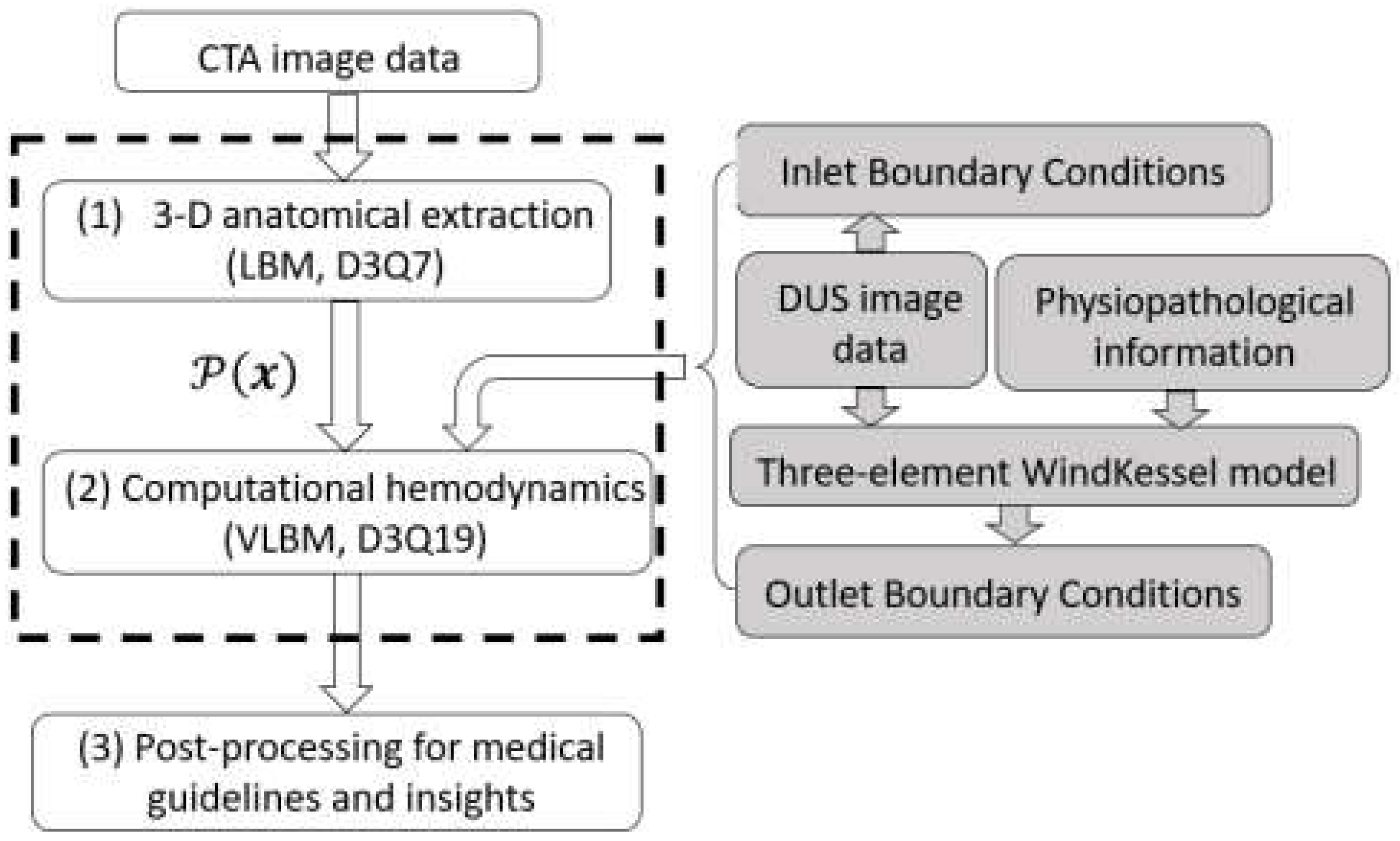
2. Methods and Materials
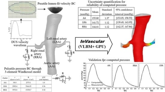
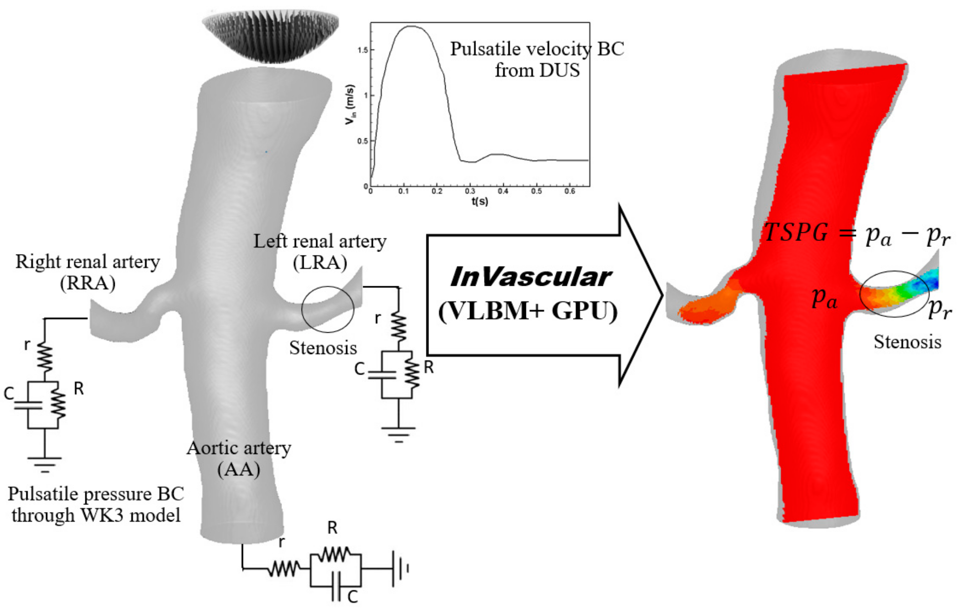
2.1. Physiological Inlet and Outlet Boundary Conditions
2.1.1. Implementation of Velocity and Pressure BCs in VLBM
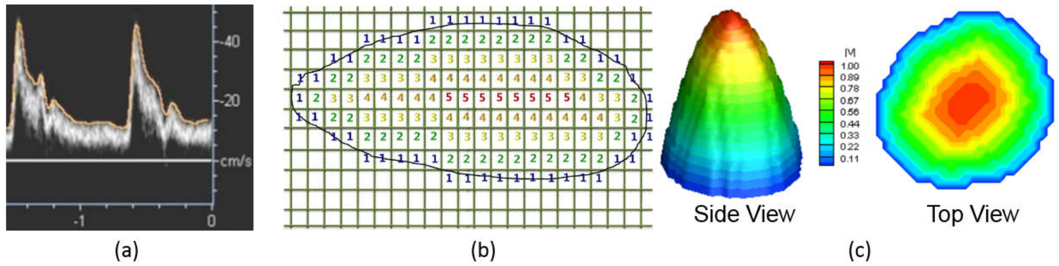
2.1.2. Lumen-Fitted Velocity BC Profile at an Inlet
- (1)
- Declare a matrix , i.e., () and initialize it as .
- (2)
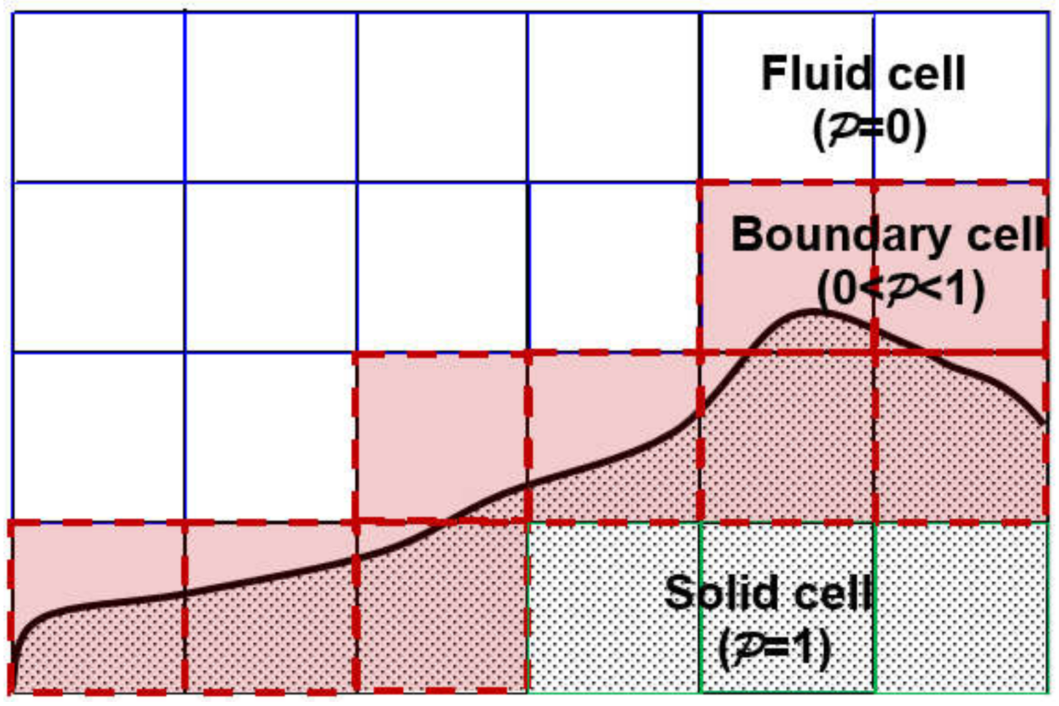
- Loop i from 1 to and j from 1 to , if
- a cell’s is neither 0 nor 1 (i.e., a boundary cell), assign for this cell and define its velocity magnitude 0,
- a cell’s is 0 (i.e., a fluid cell) and the value of any neighboring cell is 0, assign for this cell,
- a cell’s is 0 and the value of any neighboring cell is 1, assign for this cell,
- continue until all the fluid cells are assigned. The last index of the cell labeling is .
- (3)
- Loop i from 1 to and j from 1 to and define velocity magnitude as .
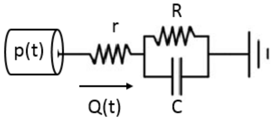
2.1.3. WK3-Based Pressure BC at an Outlet
- (1)
- Determine the total resistance in the arterial segment
- Assume the total system compliance cm5/dynes.
- Calculate the total resistance .
- (2)
- (3)
- Tune r and R based on DUS flow rate at each outlet.
- Integrate the pressure BC from the WK3, Equation (9), into VLBM, Equation (7), and run InVascular. In one pulsation, r, R, and C remain the same but Q (t) at each outlet is obtained from the simulation.
- Once a simulation is done, check if the flow rate at each outlet matches that calculated from DUS imaging data. If yes, r and R are determined; If not, adjust Rt and repeat (1) b, (2), and (3).
- (4)
- Determine the compliance C at each outlet.
- Distribute to each outlet proportional to the corresponding mean flow rate.
- Check if the mean arterial pressure matches at the inlet. If not, adjust in (1) a. and repeat (1) and (2).
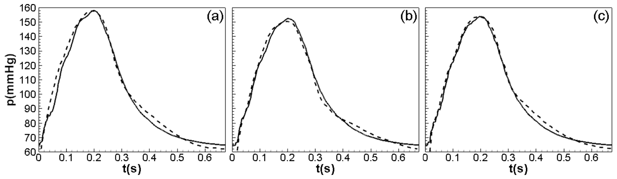
2.2. Uncertainty Quantification
2.3. Materials
3. Results
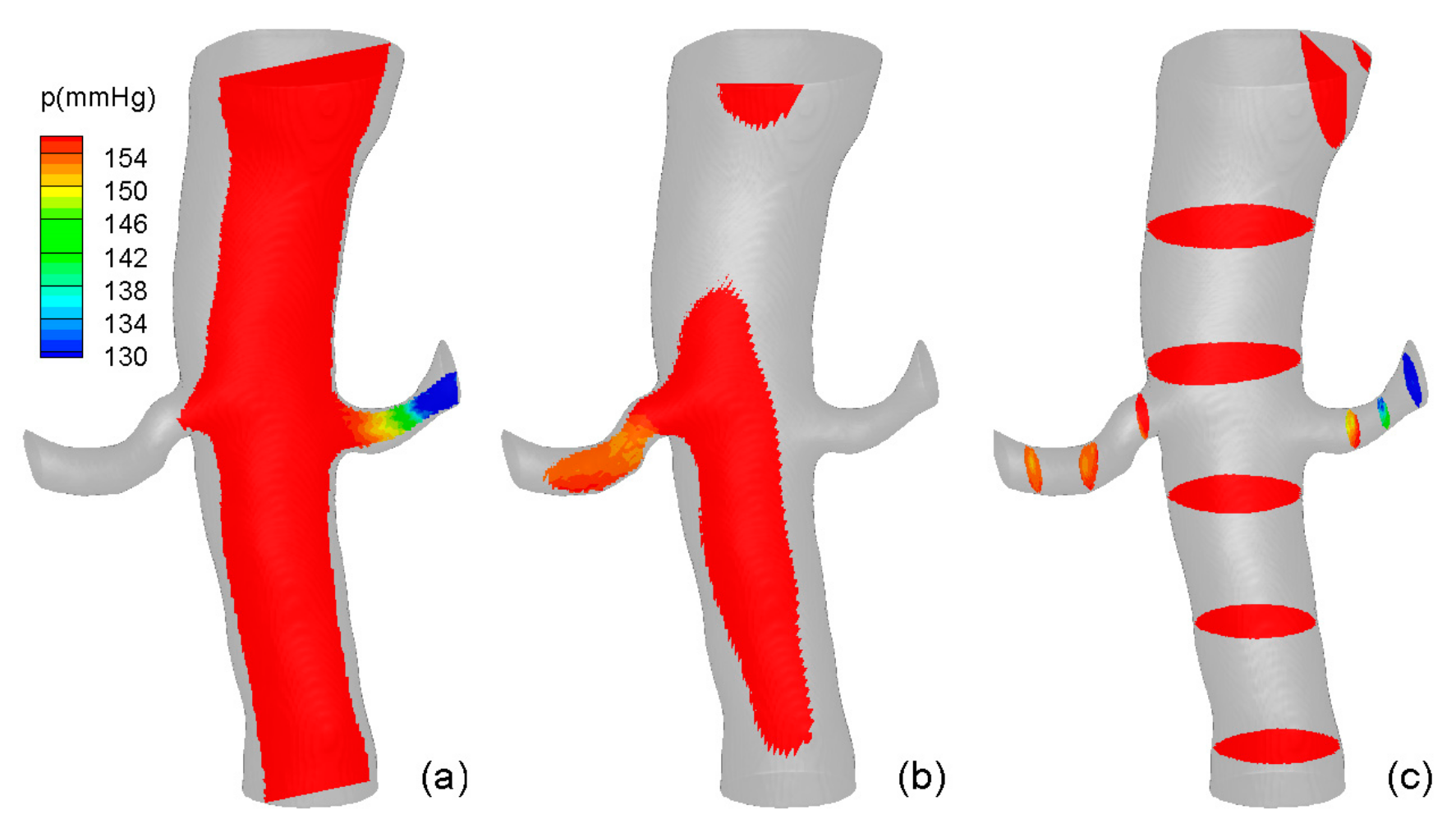
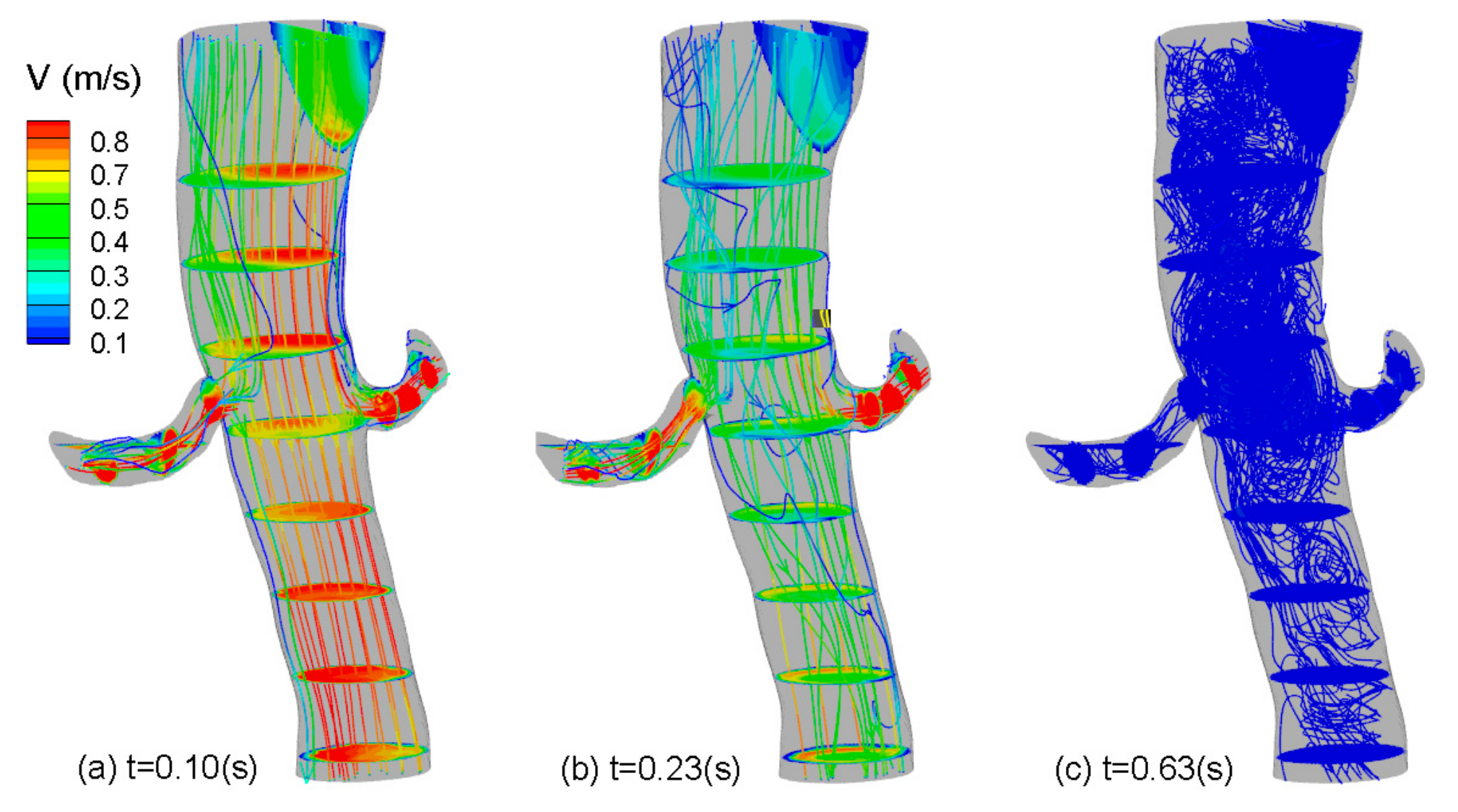
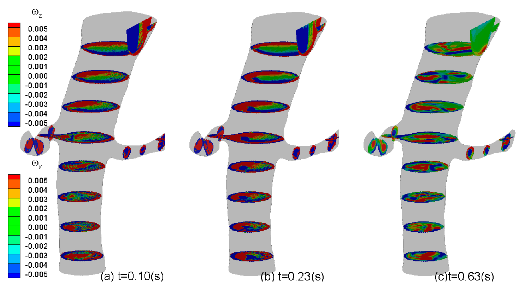
3.1. Pulsatile Hemodynamics in an Aortorenal Arterial System
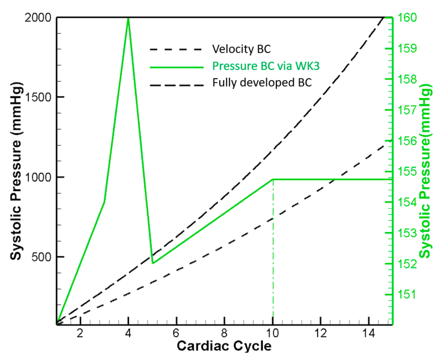
3.2. Impact of r, C, and R Parameters on Pressure Quantification
4. Discussion
Author Contributions
Funding
Institutional Review Board Statement
Informed Consent Statement
Data Availability Statement
Conflicts of Interest
Nomenclatures
| AA | Aortic Artery |
| BC | Boundary Condition |
| CFD | Computational Fluid Dynamics |
| CTA | Computed Tomography Angiography |
| DUS | Doppler Ultrasound |
| FOSM | First-Order Second Moment |
| GPU | Graphic Processing Unit |
| ICHD | Image-Based Computational Hemodynamics |
| LBM | Lattice Boltzmann Method |
| LRA | Left Renal Artery |
| MAP | Mean Arterial Pressure |
| N-S | Navier-Stokes |
| RRA | Right Renal Artery |
| TSPG | Trans-Stenotic Pressure Gradient |
| UQ | Uncertainty Quantification |
| VLBM | Volumetric Lattice Boltzmann Method |
| WK3 | Three-Element Windkessel Model |
| WSS | Wall-Shear Stress |
References
- Taylor, C.A.; Draney, M.T. Experimental and Computational Methods in Cardiovascular Fluid Mechanics. Annu. Rev. Fluid Mech. 2004, 36, 197–231. [Google Scholar] [CrossRef]
- Withey, D.J.; Koles, Z.J. A Review of Medical Image Segmentation: Methods and Available Software. Int. J. Bioelectromagn. 2008, 10, 125–148. [Google Scholar]
- Taylor, C.A.; Figueroa, C. Patient-Specific Modeling of Cardiovascular Mechanics. Annu. Rev. Biomed. Eng. 2009, 11, 109–134. [Google Scholar] [CrossRef] [PubMed] [Green Version]
- Shi, Y.; Lawford, P.; Hose, R. Review of Zero-D and 1-D Models of Blood Flow in the Cardiovascular System. Biomed. Eng. Online 2011, 10, 33. [Google Scholar] [CrossRef] [PubMed] [Green Version]
- Zhang, J.M.; Zhong, L.; Su, B.; Wan, M.; Yap, J.S.; Tham, J.P.; Chua, L.P.; Ghista, D.N.; Tan, R.S. Perspective on CFD Studies of Coronary Artery Disease Lesions and Hemodynamics: A Review. Int. J. Numer. Methods Biomed. Eng. 2014, 30, 659–680. [Google Scholar] [CrossRef]
- Marsden, A.L.; Esmaily-Moghadam, M. Multiscale Modeling of Cardiovascular Flows for Clinical Decision Support. Appl. Mech. Rev. 2015, 67, 030804. [Google Scholar] [CrossRef]
- Morris, P.D.; Narracott, A.; von Tengg-Kobligk, H.; Silva Soto, D.A.; Hsiao, S.; Lungu, A.; Evans, P.; Bressloff, N.W.; Lawford, P.V.; Hose, D.R. Computational Fluid Dynamics Modelling in Cardiovascular Medicine. Heart 2016, 102, 18–28. [Google Scholar] [CrossRef] [Green Version]
- Formaggia, L.; Lamponi, D.; Quarteroni, A. One-Dimensional Models for Blood Flow In Arteries. J. Eng. Math. 2003, 47, 251–276. [Google Scholar] [CrossRef]
- Vignon-Clementel, I.E.; Figueroa, C.; Jansen, K.; Taylor, C. Outflow Boundary Conditions For 3D Simulations of Non-Periodic Blood Flow and Pressure Fields in Deformable Arteries. Comput. Methods Biomech. Biomed. Eng. 2010, 13, 625–640. [Google Scholar] [CrossRef] [Green Version]
- Vignon-Clementel, I.E.; Figueroa, C.A.; Jansen, K.E.; Taylor, C.A. Outflow Boundary Conditions for Three-Dimensional Finite Element Modeling of Blood Flow and Pressure in Arteries. Comput. Methods Appl. Mech. Eng. 2006, 195, 3776–3796. [Google Scholar] [CrossRef]
- Vignon-Clementel, I.E.; Marsden, A.L.; Feinstein, J.A. A Primer on Computational Simulation in Congenital Heart Disease for the Clinician. Prog. Pediatric Cardiol. 2010, 30, 3–13. [Google Scholar] [CrossRef] [Green Version]
- Alastruey, J.; Parker, K.; Peiró, J.; Sherwin, S. Lumped Parameter Outflow Models for 1-D Blood Flow Simulations: Effect on Pulse Waves and Parameter Estimation. Commun. Comput. Phys. 2008, 4, 317–336. [Google Scholar]
- Stergiopulos, N.; Young, D.; Rogge, T. Computer Simulation of Arterial Flow with Applications to Arterial and Aortic Stenoses. J. Biomech. 1992, 25, 1477–1488. [Google Scholar] [CrossRef]
- Reymond, P.; Merenda, F.; Perren, F.; Rufenacht, D.; Stergiopulos, N. Validation of A One-Dimensional Model of The Systemic Arterial Tree. Am. J. Physiol.-Heart Circ. Physiol. 2009, 297, H208–H222. [Google Scholar] [CrossRef] [PubMed] [Green Version]
- Bonfanti, M.; Balabani, S.; Greenwood, J.P.; Puppala, S.; Homer-Vanniasinkam, S.; Díaz-Zuccarini, V. Computational Tools for Clinical Support: A Multi-Scale Compliant Model for Haemodynamic Simulations in an Aortic Dissection Based on Multi-Modal Imaging Data. J. R. Soc. Interface 2017, 14, 20170632. [Google Scholar] [CrossRef] [PubMed] [Green Version]
- Pirola, S.; Cheng, Z.; Jarral, O.A.; O’Regan, D.P.; Pepper, J.R.; Athanasiou, T.; Xu, X.Y. On the Choice of Outlet Boundary Conditions for Patient-Specific Analysis of Aortic Flow Using Computational Fluid Dynamics. J. Biomech. 2017, 60, 15–21. [Google Scholar] [CrossRef] [PubMed]
- Morbiducci, U.; Gallo, D.; Massai, D.; Consolo, F.; Ponzini, R.; Antiga, L.; Bignardi, C.; Deriu, M.A.; Redaelli, A. Outflow Conditions for Image-Based Hemodynamic Models of the Carotid Bifurcation: Implications for Indicators of Abnormal Flow. J. Biomech. Eng. 2010, 132, 091005. [Google Scholar] [CrossRef]
- Yu, H.; Chen, X.; Wang, Z.; Deep, D.; Lima, E.; Zhao, Y.; Shawn, D. Mass-Conserved Volumetric Lattice Boltzmann Method for Complex Flows with Willfully Moving Boundaries. Phys. Rev. E 2014, 89, 063304. [Google Scholar] [CrossRef]
- Succi, S.; Foti, E.; Higuera, F. Three-Dimensional Flows in Complex Geometries with the Lattice Boltzmann Method. Europhys. Lett. 1989, 10, 433–438. [Google Scholar] [CrossRef]
- Benzi, R.S.; Succi, S.; Vergassola, M. The Lattice Boltzmann Equation—Theory and Applications. Phys. Rep. -Rev. Sect. Phys. Lett. 1992, 222, 145–197. [Google Scholar] [CrossRef]
- An, S.; Yu, H.; Yao, J. GPU-Accelerated Volumetric Lattice Boltzmann Method for Porous Media Flow. J. Petro. Sci. Eng. 2017, 156, 546–552. [Google Scholar] [CrossRef]
- Chen, R.; Yu, H.; Zhu, L.; Taehun, L.; Patil, R. Spatial and Temporal Scaling of Unequal Microbubble Coalescence. AIChE J. 2017, 63, 1441–1450. [Google Scholar] [CrossRef] [Green Version]
- Chen, R.; Yu, H.; Zhu, L. Effects of Initial Conditions on the Coalescence of Micro-Bubbles, Proceedings of the Institution of Mechanical Engineers Part C. J. Mech. Eng. Sci. 2018, 232, 457–465. [Google Scholar] [CrossRef]
- Wang, Z.; Zhao, Y.; Sawchuck, A.P.; Dalsing, M.C.; Yu, H.W. GPU Acceleration of Volumetric Lattice Boltzmann Method for Patient-Specific Computational Hemodynamics. Comput. Fluids 2015, 115, 192–200. [Google Scholar] [CrossRef]
- Jain, K.; Jiang, J.; Strother, C.; Mardal, K.A. Transitional Hemodynamics in Intracranial Aneurysms—Comparative Velocity Investigations with High Resolution Lattice Boltzmann Simulations, Normal Resolution ANSYS Simulations, And MR Imaging. Med. Phys. 2016, 43, 6186–6198. [Google Scholar] [CrossRef]
- Groen, D.; Richardson, R.A.; Coy, R.; Schiller, U.D.; Chandrashekar, H.; Robertson, F.; Coveney, P.V. Validation of Patient-Specific Cerebral Blood Flow Simulation Using Transcranial Doppler Measurements. Front. Physiol. 2018, 9, 721. [Google Scholar] [CrossRef] [PubMed] [Green Version]
- Mirzaee, H.; Henn, T.; Krause, M.J.; Goubergrits, L.; Schumann, C.; Neugebauer, M.; Kuehne, T.; Preusser, T.; Hennemuth, A. MRI-Based Computational Hemodynamics in Patients with Aortic Coarctation Using the Lattice Boltzmann Methods: Clinical Validation Study. J. Magn. Reson. Imaging 2017, 45, 139–146. [Google Scholar] [CrossRef]
- Mokhtar, N.H.; Abas, A.; Razak, N.; Hamid, M.N.A.; Teong, S.L. Effect of Different Stent Configurations Using Lattice Boltzmann Method and Particles Image Velocimetry on Artery Bifurcation Aneurysm Problem. J. Theor. Biol. 2017, 433, 73–84. [Google Scholar] [CrossRef]
- Kang, X.; Tang, W.; Liu, S. Lattice Boltzmann Method for Simulating Disturbed Hemodynamic Characteristics of Blood Flow in Stenosed Human Carotid Bifurcation. J. Fluids Eng. 2016, 138, 121104. [Google Scholar] [CrossRef]
- An, S.; Yu, H.; Wang, Z.; Chen, R.; Kapadia, B.; Yao, J. Unified Mesoscopic Modeling and GPU-Accelerated Computational Method for Image-Based Pore-Scale Porous Media Flows. Int. J. Heat Mass Trans. 2017, 115, 1192–1202. [Google Scholar] [CrossRef]
- Yu, H.; Wang, Z.; Zhao, Y.; Sawchuk, A.P.; Lin, C.; Dalsing, M.C. GPU-accelerated Patient-Specific Computational Flow—From Radiological Images to in vivo Fluid Dynamics. In Proceedings of the 27th International Conference on Parallel Computational Fluid Dynamics Parallel CFD2015, Montreal, Canada, 30 June 2015. [Google Scholar]
- Yu, H.; Chen, R.; Wang, H.; Yuan, Z.; Zhao, Y.; An, Y.; Xu, Y.; Zhu, L. GPU Accelerated Lattice Boltzmann Simulation for Rotational Turbulence. Comput. Math. Appl. 2014, 67, 445–451. [Google Scholar] [CrossRef]
- Wolf-Gladrow, D. A Lattice Boltzmann Equation for Diffusion. J. Stat. Phys. 1995, 79, 1023–1032. [Google Scholar] [CrossRef]
- Wang, Z.; Yan, Z.; Chen, G. Lattice Boltzmann Method of Active Contour for Image Segmentation. In Proceedings of the Image and Graphics (ICIG), 2011 Sixth International Conference, Hefei, China, 12–15 August 2011; pp. 338–343. [Google Scholar]
- Sethian, J.A. Level Set Methods and Fast Marching Methods: Evolving Interfaces in Computational Geometry, Fluid Mechanics, Computer Vision, and Materials Science; Cambridge University Press: Cambridge, UK, 1999; Volume 3. [Google Scholar]
- Guo, Z.-L.; Zheng, C.-G.; Shi, B.-C. Non-Equilibrium Extrapolation Method for Velocity And Pressure Boundary Conditions In The Lattice Boltzmann Method. Chin. Phys. 2002, 11, 366. [Google Scholar]
- Westerhof, N.; Lankhaar, J.-W.; Westerhof, B.E. The Arterial Windkessel. Med. Biol. Eng. Comput. 2009, 47, 131–141. [Google Scholar] [CrossRef] [PubMed] [Green Version]
- Holenstein, R.; Ku, D.N. Reverse Flow in The Major Infrarenal Vessels–A Capacitive Phenomenon. Biorheology 1988, 25, 835–842. [Google Scholar] [CrossRef]
- Bax, L.; Woittiez, A.J.; Kouwenberg, H.J.; Mali, W.P.; Buskens, E.; Beek, F.J.; Braam, B.; Huysmans, F.T.; Schultze Kool, L.J.; Rutten, M.J.; et al. Stent Placement in Patients With Atherosclerotic Renal Artery Stenosis and Impaired Renal Function: A Randomized Trial. Ann. Intern. Med. 2009, 150, 840–848. [Google Scholar] [CrossRef] [PubMed]
- Les, A.S.; Shadden, S.C.; Figueroa, C.A.; Park, J.M.; Tedesco, M.M.; Herfkens, R.J.; Dalman, R.L.; Taylor, C.A. Quantification of Hemodynamics in Abdominal Aortic Aneurysms During Rest and Exercise Using Magnetic Resonance Imaging and Computational Fluid Dynamics. Ann. Biomed. Eng. 2010, 38, 1288–1313. [Google Scholar] [CrossRef]
- Du, X. Unified Uncertainty Analysis by the First Order Reliability Method. J. Mech. Des. 2008, 130, 091401. [Google Scholar] [CrossRef]
- Huang, B.; Du, X. Probabilistic Uncertainty Analysis by Mean-Value First Order Saddlepoint Approximation. J. Reliab. Eng. Syst. Saf. 2008, 93, 325–336. [Google Scholar] [CrossRef]
- Rosenblatt, M. Remarks on A Multivariate Transformation. Ann. Math. Stat. 1952, 23, 3. [Google Scholar] [CrossRef]


| Outlet | r (dynes×s/cm5) | R (dynes×s/cm5) | 105C (cm5/dynes) |
|---|---|---|---|
| AA | 88.0 | 2773.1 | 1.8 |
| LRA | 2982.4 | 7666.03 | 0.36 |
| RRA | 5972.8 | 15358.7 | 0.32 |
| Spatial | Temporal | ||||
|---|---|---|---|---|---|
| Grid | MAP(mmHg) | Relative Error (%) | Cycle | Relative Error (%) | |
| 170 | 100 | 1 | 150 | ||
| 180 | 87.5 | 12.5 | 3 | 154 | 2.7 |
| 190 | 89 | 1.71 | 5 | 152 | −1.3 |
| 200 | 90 | 0.34 | 10 | 155 | 2.0 |
| 210 | 90.15 | 0.19 | 15 | 155 | 0 |
| 220 | 90.20 | 0.05 | 20 | 155 | 0 |
| Computed | Measured | Computed | Measured | |
|---|---|---|---|---|
| , left | 2.5 | 2.6 | 4.1 | 4.0 |
| , right | 2.0 | 2.0 | 4.0 | 4.0 |
| Artery | Parameter | Variables | Mean | Standard Deviation | Distribution Type |
|---|---|---|---|---|---|
| AA | r(dynes×s/cm5) | 108.12 | 3.24 | Normal | |
| AA | R(dynes×s/cm5) | 3386.38 | 101.59 | Normal | |
| LRA | r(dynes×s/cm5) | 2879.76 | 86.39 | Normal | |
| LRA | R(dynes×s/cm5) | 7386.06 | 221.58 | Normal | |
| RRA | r(dynes×s/cm5) | 3306.39 | 99.19 | Normal | |
| RRA | R(dynes×s/cm5) | 8505.96 | 255.18 | Normal | |
| AA | C(cm5/dynes) | Normal | |||
| LRA | C(cm5/dynes) | Normal | |||
| RRA | C(cm5/dynes) | Normal |
| Artery | Output Variable | 95% Confidence Interval | ||
|---|---|---|---|---|
| AA | (mmHg) | 155.80 | 1.37 | [153.05, 158.55] |
| LRA | (mmHg) | 141.72 | 1.12 | [139.49, 143.95] |
| RRA | (mmHg) | 144.61 | 1.12 | [142.37, 147.86] |
| Case | |||
|---|---|---|---|
| 1 | |||
| 2 | |||
| 3 | |||
| 4 | |||
| 5 |
| Case | |||
|---|---|---|---|
| 1 | [153.05, 158.55] | [139.49, 143.95] | [142.37, 146.86] |
| 2 | [159.48, 167.74] | [150.38, 158.12] | [56.25, 56.59] |
| 3 | [154.14, 160.30] | [149.45,155.25] | [150.92,156.79] |
| 4 | [107.84, 111.58] | [104.72,108.27] | [73.37,75.62] |
| 5 | [121.28, 125.15] | [115.57, 119.11] | [99.69,104.64] |
Publisher’s Note: MDPI stays neutral with regard to jurisdictional claims in published maps and institutional affiliations. |
© 2022 by the authors. Licensee MDPI, Basel, Switzerland. This article is an open access article distributed under the terms and conditions of the Creative Commons Attribution (CC BY) license (https://creativecommons.org/licenses/by/4.0/).
Share and Cite
Yu, H.; Khan, M.; Wu, H.; Zhang, C.; Du, X.; Chen, R.; Fang, X.; Long, J.; Sawchuk, A.P. Inlet and Outlet Boundary Conditions and Uncertainty Quantification in Volumetric Lattice Boltzmann Method for Image-Based Computational Hemodynamics. Fluids 2022, 7, 30. https://doi.org/10.3390/fluids7010030
Yu H, Khan M, Wu H, Zhang C, Du X, Chen R, Fang X, Long J, Sawchuk AP. Inlet and Outlet Boundary Conditions and Uncertainty Quantification in Volumetric Lattice Boltzmann Method for Image-Based Computational Hemodynamics. Fluids. 2022; 7(1):30. https://doi.org/10.3390/fluids7010030
Chicago/Turabian StyleYu, Huidan, Monsurul Khan, Hao Wu, Chunze Zhang, Xiaoping Du, Rou Chen, Xin Fang, Jianyun Long, and Alan P. Sawchuk. 2022. "Inlet and Outlet Boundary Conditions and Uncertainty Quantification in Volumetric Lattice Boltzmann Method for Image-Based Computational Hemodynamics" Fluids 7, no. 1: 30. https://doi.org/10.3390/fluids7010030
APA StyleYu, H., Khan, M., Wu, H., Zhang, C., Du, X., Chen, R., Fang, X., Long, J., & Sawchuk, A. P. (2022). Inlet and Outlet Boundary Conditions and Uncertainty Quantification in Volumetric Lattice Boltzmann Method for Image-Based Computational Hemodynamics. Fluids, 7(1), 30. https://doi.org/10.3390/fluids7010030