Article

A Monolithic Finite Element Formulation for Magnetohydrodynamics Involving a Compressible Fluid

Department of Mechanical Engineering, Indian Institute of Science, Bangalore 560012, India
*
Author to whom correspondence should be addressed.
Fluids 2022, 7(1), 27; https://doi.org/10.3390/fluids7010027
Submission received: 12 November 2021 / Revised: 18 December 2021 / Accepted: 4 January 2022 / Published: 7 January 2022
(This article belongs to the Collection Feature Paper for Mathematical and Computational Fluid Mechanics)

Abstract

:
This work develops a new monolithic finite-element-based strategy for magnetohydrodynamics (MHD) involving a compressible fluid based on a continuous velocity–pressure formulation. The entire formulation is within a nodal finite element framework, and is directly in terms of physical variables. The exact linearization of the variational formulation ensures a quadratic rate of convergence in the vicinity of the solution. Both steady-state and transient formulations are presented for two- and three-dimensional flows. Several benchmark problems are presented, and comparisons are carried out against analytical solutions, experimental data, or against other numerical schemes for MHD. We show a good coarse-mesh accuracy and robustness of the proposed strategy, even at high Hartmann numbers.

1. Introduction

The flow of a conducting fluid in the presence of a magnetic field is termed as magnetohydrodynamics (MHD). There are several applications of MHD, including the flow of liquid metals [1,2,3,4,5,6,7,8,9,10,11,12], nanofluids [13,14,15,16,17,18], non-Newtonian fluids [19,20,21,22,23], magneto-gas dynamics [24,25,26], astrophysical fluid dynamics [27], and many biomedical devices. References [14,15] use a control-volume-based finite element strategy (CVFEM) in their formulation. References [10,11,12,24] use edge elements for discretizing the magnetic field. Ciuca et al. [26] use hybridized discontinuous Galerkin methods for ideal and resistive MHD, while Eswaran et al. [28] use a finite volume approach.
The salient features of this work are as follows:
  • Most of the MHD strategies treat the fluid as incompressible [28,29]. Since compressibility effects play a key role in applications such as magneto-gas dynamics, in this work, we focus on developing a MHD strategy for compressible fluids. Moreover, we show that the strategy works very well, even when the fluid is almost incompressible (with a stiff equation of state); thus, the same strategy can be used even when the fluid is almost incompressible;
  • We develop a monolithic strategy based on the fully coupled equations for the fluid and the magnetic fields. The inclusion of the coupling terms yields a faster rate of convergence compared to a staggered strategy, where the fluid and the magnetic field variables are solved for in a sequential manner;
  • The formulation is based on primitive flow variables, such as velocity, density, temperature, pressure, and the magnetic field, which makes the implementation simple. The treatment of the boundary conditions is also very straightforward, as these are generally specified in terms of the primitive variables or their duals;
  • In contrast to the work in references [1,2,4,5,6,7,8] that use a stabilized formulation, we use a stable formulation based on an appropriate choice of interpolations for the various field variables. We use higher order interpolation functions for the velocity and magnetic fields, as compared to the pressure, density, and temperature field variables. This ensures the satisfaction of the inf-sup stability conditions. No stabilizing terms need to be used, and no parameters need to be adjusted in the proposed formulation;
  • The governing equations for the fluid, namely the continuity, Navier–Stokes, energy, and state equations are considered in their entirety without any approximations, such as the Boussinesq approximation;
  • Joule heating effects have been included in the formulation.

2. Mathematical Formulation

2.1. Governing Equations for MHD Involving a Compressible Fluid

We first present the equations for the magnetic fields, and then the coupled equations to be solved on the entire domain.

2.1.1. Magnetic Field Equations

The Maxwell equations for electromagnetism under MHD assumptions reduce to the following set of equations [29]:
μ m H t + × E = 0 ,
· ( μ m H ) = 0 ,
× H = j ,
· j = 0 ,
where H and E represent the magnetic and electric fields, respectively, μ m is the magnetic permeability, and j is the current density. The above equations are supplemented by Ohm’s law for a conducting fluid, which is given by
j = σ e ( E + μ m u × H ) ,
where σ e and u denote the electrical conductivity and the velocity of the fluid, respectively. Combining Equations (1) and (2), we obtain the governing differential equation for H as
× × H + σ e μ m H t = σ e μ m × u × H on Ω ,
where Ω represents the fluid domain.

2.1.2. Coupled Equations for Compressible MHD

Let Ω and Γ denote the domain and its boundary, Γ t and Γ u denote the parts of boundaries where tractions and velocity are prescribed, respectively, Γ θ and Γ q represent portions of Γ where temperature and normal heat flux are prescribed, respectively, and Γ H and Γ E represent portions of the boundary where H × n and ( × H ) × n are prescribed, respectively.
We are interested in finding an approximate solution to the following initial-boundary value problem:
Determine the velocity u , density ρ , pressure p, temperature θ , magnetic field H , stresses τ , rate of deformation D , and heat flux q on the domain Ω such that
× × H + σ e μ m H t = σ e μ m × u × H ,
· ( μ m H ) = 0 ,
( ρ u ) t + ρ ( u ) u + u · ( ρ u ) = · τ + ρ b + μ m ( × H ) × H
ρ t + · ( ρ u ) = 0 ,
C v ( ρ θ ) t + ρ θ · u + u · ρ θ + θ ρ = p · u + σ : D · q + ρ Q h + | × H | 2 σ e ,
p = p ˜ ( ρ , θ ) ,
where b is the body force per unit mass, σ is the viscous stress, and C v is the specific heat at constant volume. For a Newtonian fluid, τ = p ( ρ , θ ) I + σ , where σ = λ ( tr D ) I + 2 ν D , with λ and μ denoting the viscosity coefficients. Similarly, we have q = κ θ , where κ is the thermal conductivity. The last term in Equation (4c) represents the additional body force, namely the Lorentz force μ m ( j × H ) , that acts on the fluid. A term j · E , which represents Joule heating [30], gets added to the first law of thermodynamics [31] for a fluid due to magnetic effects. After subtracting the dot product of the momentum equation given by Equation (4c) with the velocity field u from the first law of thermodynamics [32], and using the properties of the scalar triple product and Equation (2), we have
j · E μ m [ u · ( j × H ) ] = j · [ E + μ m u × H ] = j · j σ e ,
which is the last term in Equation (4e). The above governing equations are to be solved subject to appropriate initial and boundary conditions.

2.2. Variational Formulation

Denoting the variations of H , u , ρ , θ , and p with a subscript δ , the variational statements corresponding to Equation (4) can be written as
Ω σ e μ m H δ · H t d Ω + Ω × H δ · × H d Ω + Ω · H δ · H d Ω = Ω σ e μ m × H δ · u × H d Ω H δ ,
Ω u δ T ( ρ u ) t + ρ ( u ) u + u · ( ρ u ) d Ω Ω ( · u δ ) p d Ω + Ω [ D c ( u δ ) ] T C c D c d Ω = Ω ρ u δ T b d Ω + Ω μ m u δ T [ ( × H ) × H ] d Ω + Γ t u δ T t ¯ d Γ u δ ,
Ω ρ δ ρ t + ρ · u + u · ρ d Ω = 0 ρ δ ,
Ω C v θ δ ( ρ θ ) t + ρ θ · u + u · ρ θ + θ ρ d Ω + Ω θ δ p · u σ : D d Ω + Ω k θ δ · θ d Ω = Ω ρ θ δ Q h d Ω Γ q θ δ q ¯ n d Γ + Ω θ δ | × H | 2 σ e d Ω θ δ ,
Ω p δ p p ˜ ρ , θ d Ω = 0 p δ ,
where C c and D c denote the material constitutive tensor and rate of deformation tensor expressed in an engineering form as
D c = D x x D y y D z z 2 D x y 2 D y z 2 D x z , C c = λ + 2 μ λ λ 0 0 0 λ λ + 2 μ λ 0 0 0 λ λ λ + 2 μ 0 0 0 0 0 0 μ 0 0 0 0 0 0 μ 0 0 0 0 0 0 μ ,
q ¯ n is the normal heat flux prescribed on Γ q , and t ¯ is the prescribed traction on Γ t . Note that the weak implementation of the state equation given by Equation (5e) is critical in ensuring that a lower-order interpolation for the pressure can be used in order to satisfy the inf-sup conditions, which would otherwise be dictated by the interpolations being used for the density and temperature. Equation (5a) has been derived using a penalty term of the type ( · H ) 2 , as shown in [29]. In addition, the term
Γ H H δ × n · σ e μ m u × H × H d Γ = Γ H σ e ( H δ × n ) · E d Γ ,
has been excluded from Equation (5a), since, in the problems that we consider here, either H × n is specified on the boundary, or the surface is purely conducting.

2.3. Time Stepping Strategy

The time discretization on the time interval [ t n , t n + 1 ] is carried out by using the following general trapezoidal rule:
σ e μ m Ω H δ · H n + 1 H n t Δ d Ω Ω ( × H δ ) · ( u × H ) α d Ω + Ω ( × H δ ) · ( × H α ) d Ω + Ω ( · H δ ) ( · H α ) d Ω = 0 H δ ,
Ω u δ · ( ρ u ) n + 1 ( ρ u ) n t Δ + [ ρ ( u ) u ] α + [ u · ( ρ u ) ] α d Ω + Ω [ D c ( u δ ) ] T C c ( D c ) α d Ω Ω ( · u δ ) p α d Ω = Ω ( ρ u δ T b ) α d Ω + Γ ( u δ T t ¯ ) α d Γ + Ω μ m u δ T [ ( × H ) × H ] α d Ω u δ ,
Ω ρ δ ρ n + 1 ρ n t Δ + ( ρ · u ) α + [ u · ( ρ ) ] α d Ω = 0 ρ δ ,
Ω C v θ δ ( ρ θ ) n + 1 ( ρ θ ) n t Δ + ( ρ θ · u ) α + [ u · ( ρ θ + θ ρ ) ] α + Ω θ δ · [ k θ ] α d Ω + Ω θ δ p α · u n + 1 + · u n 2 d Ω Ω θ δ σ α : D c ( u n + 1 ) + D c ( u n ) 2 d Ω = Ω θ δ ρ α Q h d Ω + Ω θ δ | × H | α 2 σ e d Ω Γ q θ δ q ¯ α d Γ θ δ ,
where β α = ( 1 α ) β n + α β n + 1 for any field variable β .

2.4. Linearization

A Newton–Raphson strategy is developed by linearizing the above equations. Let ( u k , ρ k , θ k , p k , H k ) and ( u k + 1 , ρ k + 1 , θ k + 1 , p k + 1 , H k + 1 ) represent the values of the velocity, density, temperature, pressure, and magnetic field, respectively, at the k’th and k + 1 ’th iterations at time step n + 1 . Let ( u Δ , ρ Δ , θ Δ , p Δ , H Δ ) denote the increments in the respective field variables. The chain and product rules are applied to obtain the linearized form of Equation (6) as follows:
σ e μ m Ω H δ T H Δ d Ω + α t Δ { Ω ( · H δ ) ( · H Δ ) + ( × H δ ) · ( × H Δ ) d Ω σ e μ m Ω ( × H δ ) · ( u k × H Δ ) d Ω + σ e μ m Ω ( × H δ ) · ( H k × u Δ ) d Ω } = σ e μ m Ω H δ T H n H k d Ω + α t Δ { σ e μ m Ω ( × H δ ) · ( u k × H k ) d Ω Ω [ ( × H δ ) · ( × H k ) ( · H ) ( · H k ) ] d Ω } + ( 1 α ) t Δ { σ e μ m Ω ( × H δ ) · ( u n × H n ) d Ω Ω [ ( × H δ ) · ( × H n ) ( · H δ ) ( · H n ) ] d Ω } H δ ,
Ω u δ T ρ k u Δ d Ω + Ω u δ T u k ρ Δ d Ω + α t Δ { Ω u δ T [ ρ k ( u k ) u Δ + ρ k ( u Δ ) u k + u k · ( ρ k u Δ ) + · ( ρ k u k ) u Δ ] d Ω + Ω [ D c ( u δ ) ] T C c [ D c ( u Δ ) ] d Ω + Ω [ D c ( u δ ) ] T C c D c ( u k ) θ Δ d Ω + Ω u δ T [ u k · ( u k ρ Δ ) + ( u k ) u k ρ Δ b ρ Δ ] d Ω Ω μ m u δ T [ ( × H k ) × H Δ H k × ( × H Δ ) ] d Ω Ω ( · u δ ) p Δ d Ω } = Ω u δ T [ ρ k u k ρ n u n ] + α t Δ { Γ t u δ T t ¯ k d Γ + Ω u δ T [ ρ k b ρ k ( u k ) u k u k · ( ρ k u k ) + μ m ( × H k ) × H k ] d Ω Ω [ D c ( u δ ) ] T τ c k d Ω } + ( 1 α ) t Δ { Γ t u δ T t ¯ n d Γ + Ω u δ T [ ρ n b ρ n ( u n ) u n u n · ( ρ n u n ) + μ m ( × H n ) × H n ] d Ω Ω [ D c ( u δ ) ] T τ c n d Ω } u δ ,
Ω ρ δ ρ Δ d Ω + α t Δ [ Ω ρ δ ρ k ( · u Δ ) + ( ρ k ) · u Δ d Ω + Ω ρ δ [ ( · u k ) ρ Δ + u k · ( ρ Δ ) ] d Ω ] = α t Δ Ω ρ δ · ( ρ k u k ) d Ω ( 1 α ) t Δ Ω ρ δ · ( ρ n u n ) d Ω Ω ρ δ ρ k ρ n d Ω ρ δ ,
t Δ 2 Ω θ δ [ ( α p k + ( 1 α ) p n ) · u Δ [ D c ( u n ) ] T C c D c ( u Δ ) 2 α [ D c ( u k ) ] T C c D c ( u Δ ) ] d Ω + Ω C v θ δ θ k ρ Δ d Ω + Ω C v θ δ ρ k θ Δ d Ω α t Δ 2 Ω θ δ [ D c ( u k ) ] T C c [ D c ( u k ) + D c ( u n ) ] θ Δ d Ω + α t Δ 2 Ω θ δ [ · u k + · u n ] p Δ d Ω + α t Δ { Ω C v θ δ [ ρ k θ k ( · u Δ ) + ( ρ k θ k + θ k ρ k ) · u Δ ] d Ω + Ω C v θ δ [ u k . θ k ρ Δ + ( · u k ) θ k ρ Δ + θ k ( u k ) T ρ Δ ] d Ω Ω θ δ Q h ρ Δ d Ω + Ω C v θ δ [ ρ k ( · u k ) θ Δ + ( ρ k · u k ) θ Δ + ρ k ( u k · θ Δ ) ] d Ω + Ω θ δ · [ k f θ Δ + k f θ k θ Δ ] d Ω 2 σ e Ω θ δ ( × H k ) · ( × H Δ ) d Ω } = α t Δ { Ω θ δ [ ρ k Q h + | × H k | 2 σ e C v [ ρ k θ k ( · u k ) + u k · ( ρ k θ k + θ k ρ k ) ] ] d Ω Ω k f θ δ · θ k d Ω Γ θ δ q ¯ k d Γ } + ( 1 α ) t Δ { Ω θ δ ρ n Q h + | × H n | 2 σ e C v [ ρ n θ n ( · u n ) + u n · ( ρ n θ n + θ n ρ n ) ] d Ω Ω k f θ δ · θ n d Ω Γ θ δ q ¯ n d Γ } α t Δ 2 Ω θ δ [ τ c k ] T D c ( u k ) + D c ( u n ) d Ω + ( 1 α ) t Δ 2 Ω θ δ [ τ c n ] T D c ( u k ) + D c ( u n ) d Ω Ω c v θ δ [ ρ k θ k ρ n θ n ] d Ω θ δ ,
α t Δ Ω p δ p Δ p ˜ ρ k ρ Δ p ˜ θ k θ Δ d Ω = α t Δ Ω p δ p k p ˜ ( ρ k , θ k ) d Ω p δ ,
where k f and C c denote the derivatives of k f and C c with respect to θ .

2.5. Finite Element Formulation

Let the magnetic field, velocity, density, temperature, pressure fields, and their variations and increments be interpolated as
H = N H ^ , u = N u ^ , ρ = N ρ ρ ^ , θ = N θ θ ^ , p = N p p ^ , H δ = N H ^ δ , u δ = N u ^ δ , ρ δ = N ρ ρ ^ δ , θ δ = N θ θ ^ δ , p δ = N p p ^ δ , H Δ = N H ^ Δ , u Δ = N u ^ Δ , ρ Δ = N ρ ρ ^ Δ , θ Δ = N θ θ ^ Δ , p Δ = N p p ^ Δ .
In the case of the 27-noded hexahedral element, the shape functions N for u and H are the standard triquadratic Lagrange interpolation functions, while the density, temperature, and pressure fields are interpolated using a trilinear continuous interpolation in order to obtain a stable discretization. We thus have
D c ( u Δ ) = B u ^ Δ , ( u Δ ) u k = R B N L u ^ Δ , · u Δ = B p u ^ Δ , ρ k ( · u Δ ) + ( ρ k ) · u Δ = B ρ 1 u ^ Δ , ( · u k ) ρ Δ + u k · ( ρ Δ ) = B ρ 2 ρ ^ Δ , θ Δ = B θ θ ^ Δ , × H Δ = B H H ^ Δ , · H Δ = B p H ^ Δ ,
where
B = N 1 , x 0 0 N 2 , x 0 0 . . . 0 N 1 , y 0 0 N 2 , y 0 . . . 0 0 N 1 , z 0 0 N 2 , z . . . N 1 , y N 1 , x 0 N 2 , y N 2 , x 0 . . . 0 N 1 , z N 1 , y 0 N 2 , z N 2 , y . . . N 1 , z 0 N 1 , x N 2 , z 0 N 2 , x . . . , B p = N 1 , x N 1 , y N 1 , z N 2 , x N 2 , y N 2 , z . . . , R = u x k u y k u z k 0 0 0 0 0 0 0 0 0 u x k u y k u z k 0 0 0 0 0 0 0 0 0 u x k u y k u z k , B N L = N 1 , x 0 0 N 2 , x 0 0 . . . N 1 , y 0 0 N 2 , y 0 0 . . . N 1 , z 0 0 N 2 , z 0 0 . . . 0 N 1 , x 0 0 N 2 , x 0 . . . 0 N 1 , y 0 0 N 2 , y 0 . . . 0 N 1 , z 0 0 N 2 , z 0 . . . 0 0 N 1 , x 0 0 N 2 , x . . . 0 0 N 1 , y 0 0 N 2 , y . . . 0 0 N 1 , z 0 0 N 2 , z . . . , B H = 0 N 1 , z N 1 , y 0 N 2 , z N 2 , y . . . N 1 , z 0 N 1 , x N 2 , z 0 N 2 , x . . . N 1 , y N 1 , x 0 N 2 , y N 2 , x 0 . . . , B ρ 1 = ρ k N 1 , x + ρ k x N 1 ρ k N 1 , y + ρ k y N 1 ρ k N 1 , z + ρ k z N 1 ρ k N 2 , x + ρ k x N 2 . . . , B ρ 2 = ( · u k ) N 1 + ( u k · ) N 1 ( · u k ) N 2 + ( u k · ) N 2 . . . , B ρ = B θ = N 1 , x N 2 , x . . . N 1 , y N 2 , y . . . N 1 , z N 2 , z . . . .
The various cross-product terms occurring in the formulation are discretized as follows:
u k × H Δ = u mat k N H ^ Δ , H k × u Δ = H mat k N u ^ Δ , u k × H k = H mat k u k , u n × H n = H mat n u n , G k = × H k , ( × H k ) × H k = H mat k G k , ( × H n ) × H n = H mat n G n , H k × ( × H Δ ) = H mat k B H H ^ Δ ,
where
u mat k = 0 u 3 k u 2 k u 3 k 0 u 1 k u 2 k u 1 k 0 , u mat n = 0 u 3 n u 2 n u 3 n 0 u 1 n u 2 n u 1 n 0 , H mat k = 0 H 3 k H 2 k H 3 k 0 H 1 k H 2 k H 1 k 0 , H mat n = 0 H 3 n H 2 n H 3 n 0 H 1 n H 2 n H 1 n 0 , G mat k = 0 G 3 k G 2 k G 3 k 0 G 1 k G 2 k G 1 k 0 .
Using the arbitrariness of the variations, the matrix form of the incremental Equation (7) can be written as
( M + α t Δ K k ) h ^ Δ = α t Δ f Δ k + ( 1 α ) t Δ f Δ n + g ,
where
M = M H H 0 0 0 0 0 M u u M u ρ 0 0 0 0 M ρ ρ 0 0 0 M θ u M θ ρ M θ θ M θ p 0 0 0 0 0 , K = K H H K H u 0 0 0 K u H K u u K u ρ K u θ K u p 0 K ρ u K ρ ρ 0 0 K θ H K θ u K θ ρ K θ θ K θ p 0 0 K p ρ K p θ K p p , h ^ Δ = H ^ Δ u ^ Δ ρ ^ Δ θ ^ Δ p ^ Δ , f Δ k = f H f u f ρ f θ f p k , f Δ n = f H f u f ρ f θ 0 n , g = g H g u g ρ g θ 0 ,
with
M H H = Ω σ e μ m N T N d Ω , M u u = Ω ρ k N T N d Ω , M u ρ = Ω N T u k N ρ d Ω , M ρ ρ = Ω N ρ T N ρ d Ω , M θ u = t Δ 2 Ω [ ( 1 α ) p n α p k ] N θ T B p d Ω t Δ 2 Ω N θ T D c T ( u n ) C c B d Ω + α t Δ Ω N θ T D c T ( u k ) C c B d Ω , M θ ρ = Ω C v θ k N θ T N ρ d Ω , M θ θ = Ω ρ k C v N θ T N θ d Ω α t Δ 2 Ω N θ T D c T ( u k ) C c D c ( u n ) D c ( u k ) N θ d Ω , M θ p = α t Δ 2 Ω N θ T · u n · u k N p d Ω , K H H = Ω [ B H T B H + B p T B p ] d Ω σ e μ m Ω B H T u mat k N d Ω , K H u = σ e μ m Ω B H T H mat k N d Ω , K u H = Ω μ m N T H mat k B H G mat k N d Ω , K u u = Ω ρ k N T ( u k ) N + R B N L d Ω + Ω B T C c B d Ω + Ω N T u k ( ρ k ) T N + ρ k B p + ( ρ k ) · u k + ρ k ( · u k ) N T N d Ω , K u ρ = Ω N T ( u k ) u k b N ρ d Ω + Ω N T u k ( u k ) T B ρ + ( · u k ) u k N ρ d Ω , K u θ = Ω B T C c D c ( u k ) N θ d Ω , K u p = Ω B p T N p d Ω , K ρ u = Ω N ρ T B ρ 1 d Ω , K ρ ρ = Ω N ρ T B ρ 2 d Ω , K θ H = 2 σ e Ω N θ T ( G k ) T B H d Ω , K θ u = Ω C v N θ T θ k ρ k + ρ k θ k T N + ρ k θ k B p d Ω + Ω N θ T [ p k B p 2 D c T ( u k ) C c B ] d Ω , K θ ρ = Ω C v N θ T θ k ( u k ) T B ρ + θ k ( · u k ) N ρ + u k · ( θ k ) N ρ d Ω Ω Q h N θ T N ρ d Ω , K θ θ = Ω C v N θ T [ ρ k ( u k ) T B θ + ( ρ k ) · u k + ρ k ( · u k ) ] N θ d Ω + Ω [ k f B θ T B θ + k f B θ T θ k N θ N θ T D c T ( u k ) C c D c ( u k ) N θ ] d Ω , K θ p = Ω ( · u k ) N θ T N p d Ω , K p ρ = Ω p ˜ ρ k N p T N ρ d Ω , K p θ = Ω p ˜ θ k N p T N θ d Ω , K p p = Ω N p T N p d Ω , f H k = Ω [ B H T ( × H k ) + B p T ( · H k ) ] d Ω σ e μ m Ω B H T H mat k u k d Ω , f u k = Ω { N T ρ k b ρ k ( u k ) u k ( ρ k ) · u k + ( · u k ) ρ k u k μ m H mat k G k B T τ c k } d Ω + Γ N T t ¯ k d Γ , f ρ k = Ω N ρ T ρ k ( · u k ) + u k · ( ρ k ) d Ω , f θ k = Ω { ρ k N θ T Q h k f B θ T θ k C v ( θ k ρ k + ρ k θ k ) · u k + ρ k θ k ( · u k ) N θ T + ( τ c k ) T [ D c ( u k ) ] N θ T } d Ω Γ q N θ T q ¯ k d Γ + Ω ( G k ) T ( G k ) σ e N θ d Ω , f p k = Ω p k p ˜ ( ρ k , θ k ) N p T d Ω , f H n = Ω [ B H T ( × H n ) + B p T ( · H n ) ] d Ω σ e μ m Ω B H T H mat n u n d Ω , f u n = Ω { N T ρ n b ρ n ( u n ) u n ( ρ n ) · u n + ( · u n ) ρ n u n μ m H mat n G n B T τ c n } d Ω + Γ N T t ¯ n d Γ , f ρ n = Ω N ρ T ρ n ( · u n ) + u n · ( ρ n ) d Ω , f θ n = Ω { ρ n N θ T Q h k f B θ T θ n C v ( θ n ρ n + ρ n θ n ) · u n + ρ n θ n ( · u n ) N θ T + ( τ c n ) T [ D c ( u n ) ] N θ T } d Ω Γ q N θ T q ¯ n d Γ + Ω ( G n ) T ( G n ) σ e N θ d Ω , g H = σ e μ m Ω N T ( H k H n ) d Ω , g u = Ω N T [ ρ k u k ρ n u n ] d Ω , g ρ = Ω N ρ T ( ρ k ρ n ) d Ω , g θ = Ω C v ρ k θ k ρ n θ n N θ T d Ω + t Δ 2 Ω N θ T [ ( 1 α ) τ c n α τ c k ] [ D c ( u k ) D c ( u n ) ] d Ω .
The corresponding steady-state solution can be obtained directly without time stepping by solving
K k h ^ Δ = f Δ k ,

2.6. Two-Dimensional Formulation

In the case of two-dimensional flows in the x-y plane, only ( × H ) z is non-zero, and is given by
( × H ) z = H y H x .
The velocity, magnetic field, rate of deformation tensor, and constitutive tensor are given by
u = u x u y , H = H x H y , D c = D x x D y y 2 D x y , C c = λ + 2 μ λ 0 λ λ + 2 μ 0 0 0 μ ,
whereas the other matrices are as follows:
B = N 1 , x 0 N 2 , x 0 . . . 0 N 1 , y 0 N 2 , y . . . N 1 , y N 1 , x N 2 , y N 2 , x . . . , B p = N 1 , x N 1 , y N 2 , x N 2 , y . . . , R = u x k u y k 0 0 0 0 u x k u y k , B N L = N 1 , x 0 N 2 , x 0 . . . N 1 , y 0 N 2 , y 0 . . . 0 N 1 , x 0 N 2 , x . . . 0 N 1 , y 0 N 2 , y . . . , B ρ 1 = ρ k N 1 , x + ρ k x N 1 ρ k N 1 , y + ρ k y N 1 ρ k N 2 , x + ρ k x N 2 ρ k N 2 , y + ρ k y N 2 . . . , B ρ 2 = ( · u k ) N 1 + ( u k · ) N 1 ( · u k ) N 2 + ( u k · ) N 2 . . . , B θ = N 1 , x N 2 , x . . N 1 , y N 2 , y . . , B H = N 1 , y N 1 , x N 2 , y N 2 , x . . . .
The cross-product terms in the two-dimensional formulation are as follows:
H Δ × u k = [ u x k u y k ] S H ^ Δ , H k × u Δ = [ H x k H y k ] S u ^ Δ , u k × H k = [ u x k u y k ] H y k H x k , ( × H k ) × H k = ( × H k ) z H y k H x k , H k × ( × H Δ ) = H y k H x k B H H ^ Δ , u Δ × ( × H k ) = ( × H k ) z S u ^ Δ , ( × H k ) × H Δ = ( × H k ) z S H ^ Δ ,
where
S = 0 N 1 0 N 2 . . . 0 N 9 N 1 0 N 2 0 . . . N 9 0 .
Transient and steady-state solutions are obtained from Equations (8) and (9), respectively, where the relevant matrices are now given by
K u H = Ω μ m N T ( × H k ) z S + H y k H x k B H d Ω , K θ H = 2 σ e Ω ( × H k ) z N θ T B H d Ω , K H u = σ e μ m Ω B H T H x k H y k S d Ω , K H H = Ω [ B H T B H + B p T B p ] d Ω σ e μ m Ω B H T u x k u y k S d Ω , f H k = Ω [ ( × H k ) z B H T + B p T ( · H k ) ] d Ω + σ e μ m Ω B H T u x k u y k T H y k H x k d Ω , f u k = Ω { N T ρ k b ρ k ( u k ) u k ( ρ k ) · u k + ( · u k ) ρ k u k μ m ( × H k ) z H y k H x k B T τ c k } d Ω + Γ N T t ¯ k d Γ , f θ k = Ω { ρ k N θ T Q h k f B θ T θ k C v ( θ k ρ k + ρ k θ k ) · u k + ρ k θ k ( · u k ) N θ T + ( τ c k ) T [ D c ( u k ) ] N θ T } d Ω Γ q N θ T q ¯ k d Γ + Ω | ( × H k ) z | 2 σ e N θ d Ω .

3. Numerical Examples

We now demonstrate the robust performance of the developed strategy by means of several two and three-dimensional examples.

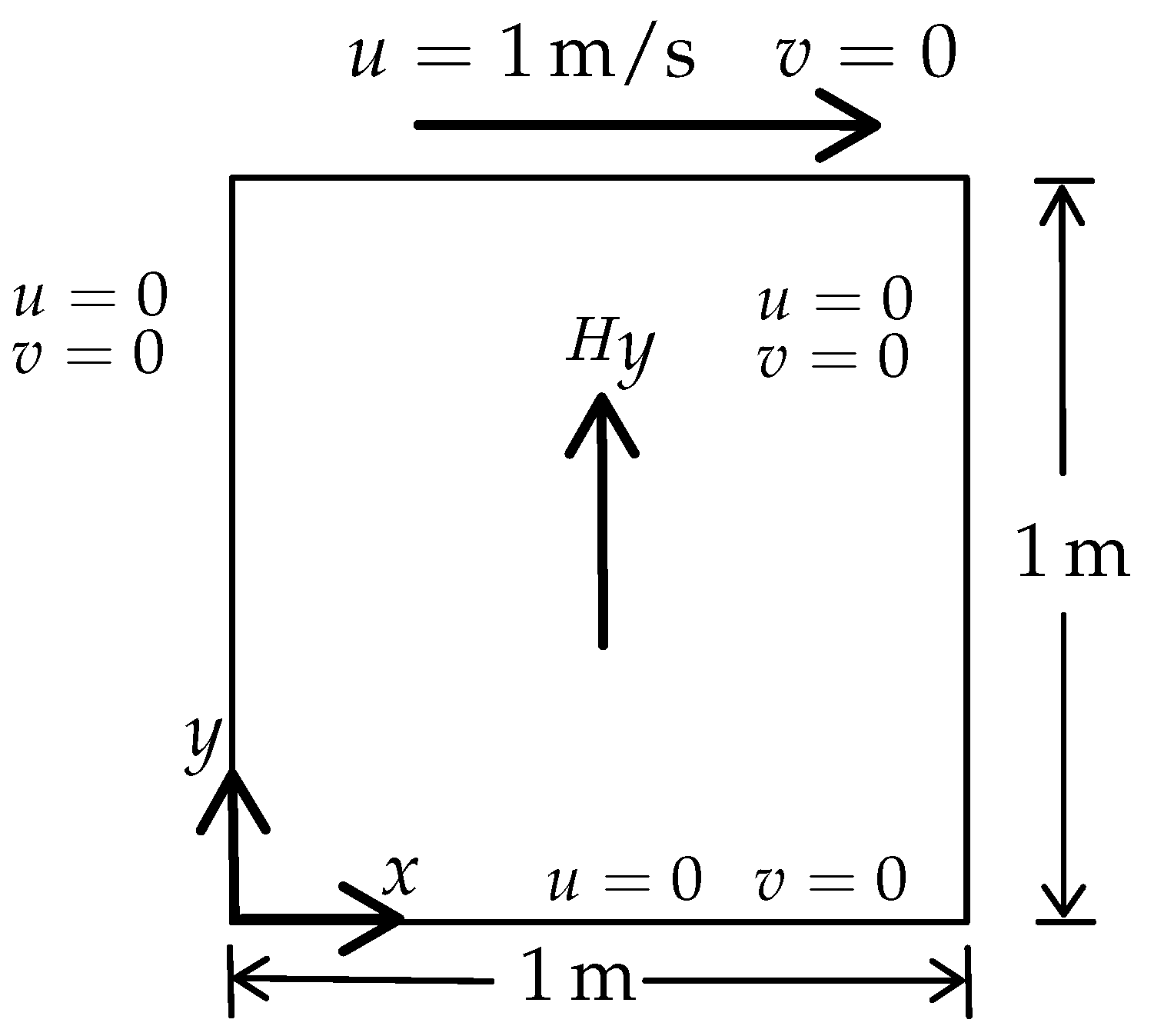
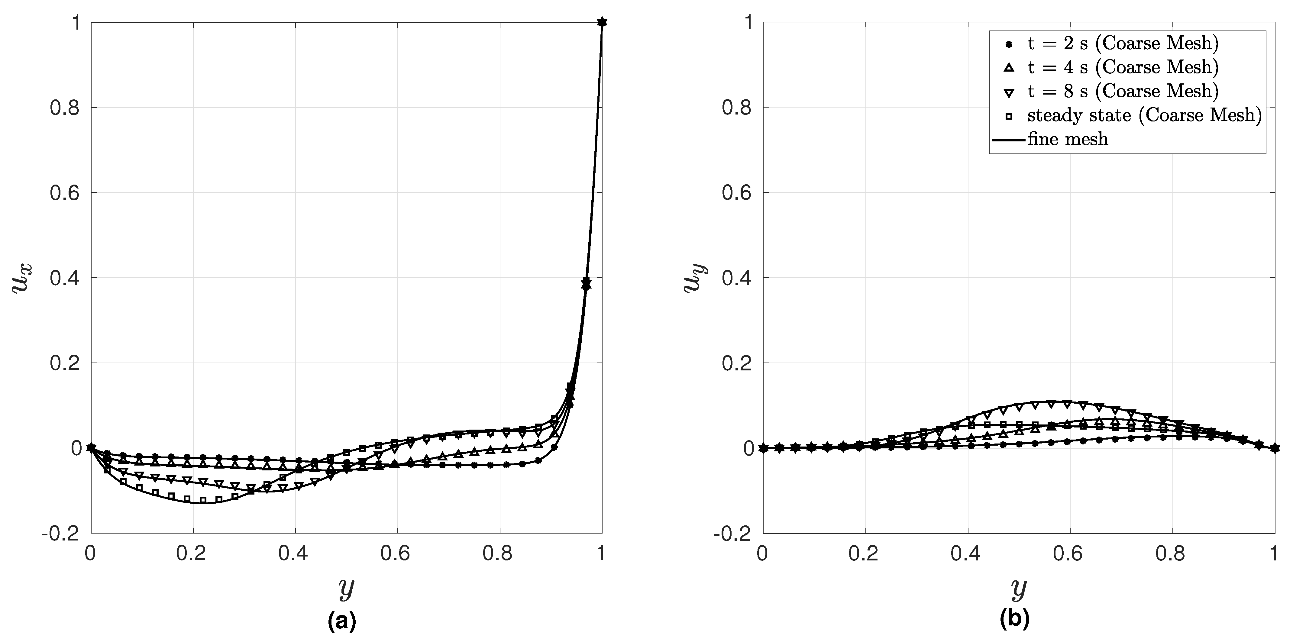
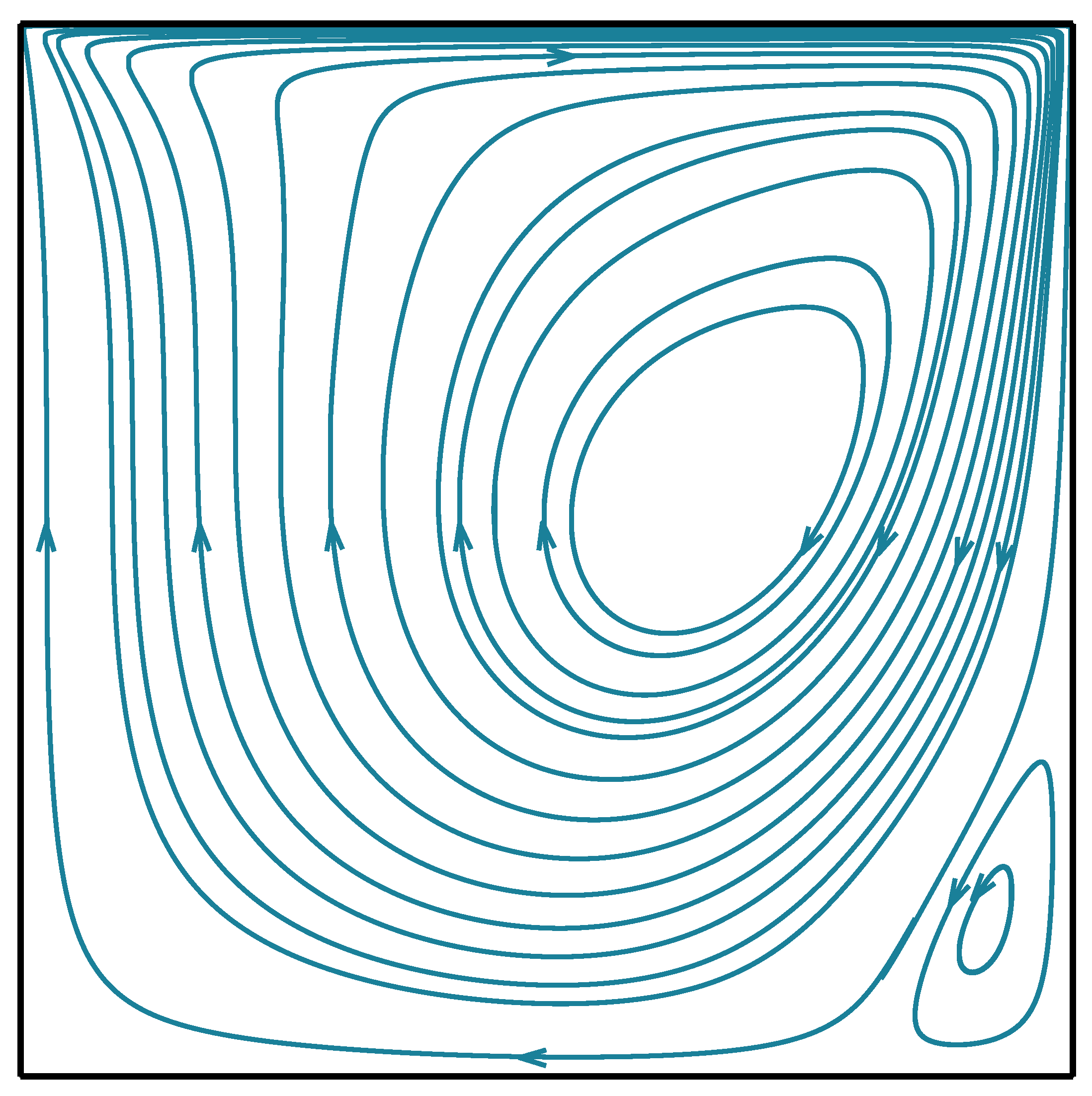
3.1. 2D Lid-Driven Cavity Problem in the Presence of a Magnetic Field

The domain of the problem is a square of dimension h = 1 m . The schematic for this problem is shown in Figure 1.
At time t = 0 , the top surface moves with a velocity u 0 = 1 m / s . A uniform magnetic field is applied throughout the domain at all times, such that H = 2 e y A / m . The magnetic field component H x is prescribed to be zero at the top and bottom surfaces at all times. The properties of the conducting fluid used for this example are μ r = 7.9577 × 10 7 , σ e = 0.01 ( Ω - m ) 1 , μ = 1.0 kg / ms , ρ = 1000 kg / m 3 corresponding to Re = 1000 , Re m = 1 and Ha = 20 , where
Re = ρ u 0 h μ , Re m = μ m σ e u 0 h , Ha = σ e μ B 0 h , B 0 = μ m H y , μ m = μ r μ 0 , μ 0 = 4 π × 10 7 .
Three different uniform meshes of nine-noded quadrilateral elements have been used to mesh the geometry, as shown in Table 1, to study the convergence of the solution with respect to mesh refinement. Ten loadsteps have been used for conducting the steady-state analyses. At every loadstep, convergence is achieved within a maximum of six iterations for all of the meshes considered. In the transient case, convergence is achieved within five iterations at each time step. The trapezoidal rule parameter α in the transient analysis is chosen as 0.5 . The solution obtained using a 120 × 120 mesh and a time step of 0.125 s is used as the reference solution. In Table 1, the error norm E steady is calculated on the basis of the computed steady-state velocity component u x along the midplane x = 0.5 as
E steady = | u reference u | x = 0.5 2 ,
where the summation is over the number of nodal points along the midplane. For the transient case, we have calculated the error as the average of the above-mentioned error measure over the first 5 seconds. From Figure 2, the rate of convergence of the error is found to be approximately equal to 1.360 and 1.084 for the steady and transient cases, respectively.
Figure 3 presents the variation of the velocity components u x and u y as a function of y at the midplane x = 0.5 m , whereas Figure 4 presents the streamlines corresponding to the steady-state solution.

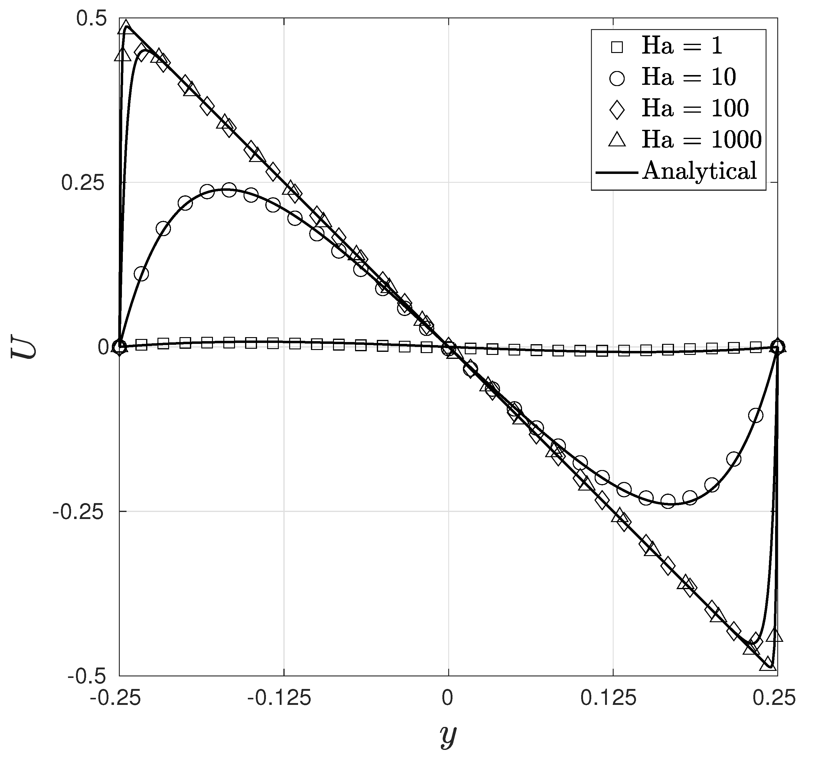
3.2. Hartman–Poiseuille Flow

This is one of the standard benchmark problems used in the literature. A conducting fluid flows between two parallel plates under the influence of a pressure gradient given by ρ G , and a magnetic field perpendicular to the two plates H = ( B o / μ m ) e y . The analytical solution for an incompressible fluid is given by [33].
u x = V 1 cosh ( Ha η ) cosh ( Ha ) , u y = 0 , u z = 0 , p = ρ G x μ H x 2 2 , H x = B o Re m sinh ( Ha η ) μ m Ha cosh ( Ha ) 1 + E B o V B o Re m η μ m , H y = B o μ m , H z = 0 ,
where Re m = μ m σ e V h , Ha = B o h σ e / μ and η = y / h .
Depending on whether the walls are insulating or conducting, the constants V and E in Equation (10) are given by
V = ρ G Ha σ e B o 2 tanh ( Ha ) , E = ρ G σ B o 1 Ha tanh ( Ha ) ( Insulating walls ) , V = ρ G σ e B o 2 , E = 0 ( Perfectly conducting walls ) .
Since the above analytical solution is for an incompressible fluid, we use water as the fluid, with the equation of state as given in [34]. The data used are the same as in [5,29], namely μ r = 9.2878 , σ e = 7.14 × 10 5 ( Ω - m ) 1 , μ = 1.5 × 10 4 kg / ms , ρ G = 4.85 × 10 5 N / m 3 , B o = 1.4494 × 10 5 Wb / m 2 , which correspond to Ha = 5 .
We use the following boundary conditions in our simulation, which correspond to the perfectly insulating case: At y = ± 0.5 , we have u = 0 , H x = 0 , and T = 293.15 K , whereas at x = 0 , 1 , the traction corresponding to a uniform pressure, and H y = B 0 / μ m , are imposed. We use a 2 × 64 element mesh for Ha = 1 , 2 , 5 , 10 , 20 and 100. Figure 5 shows almost an exact match of the numerical results obtained with the analytical solution. Convergence is achieved within the first four iterations for all of the Hartmann numbers. The same problem has been solved by Nizar [6] using a mesh of 1600 nodes, by Shadid et al. [1] using a 200 × 200 element mesh for Ha = 20 , and by Eswaran et al. [28] using a mesh of 5151 nodes, whereas, in the present formulation, only a 645 node mesh is used.

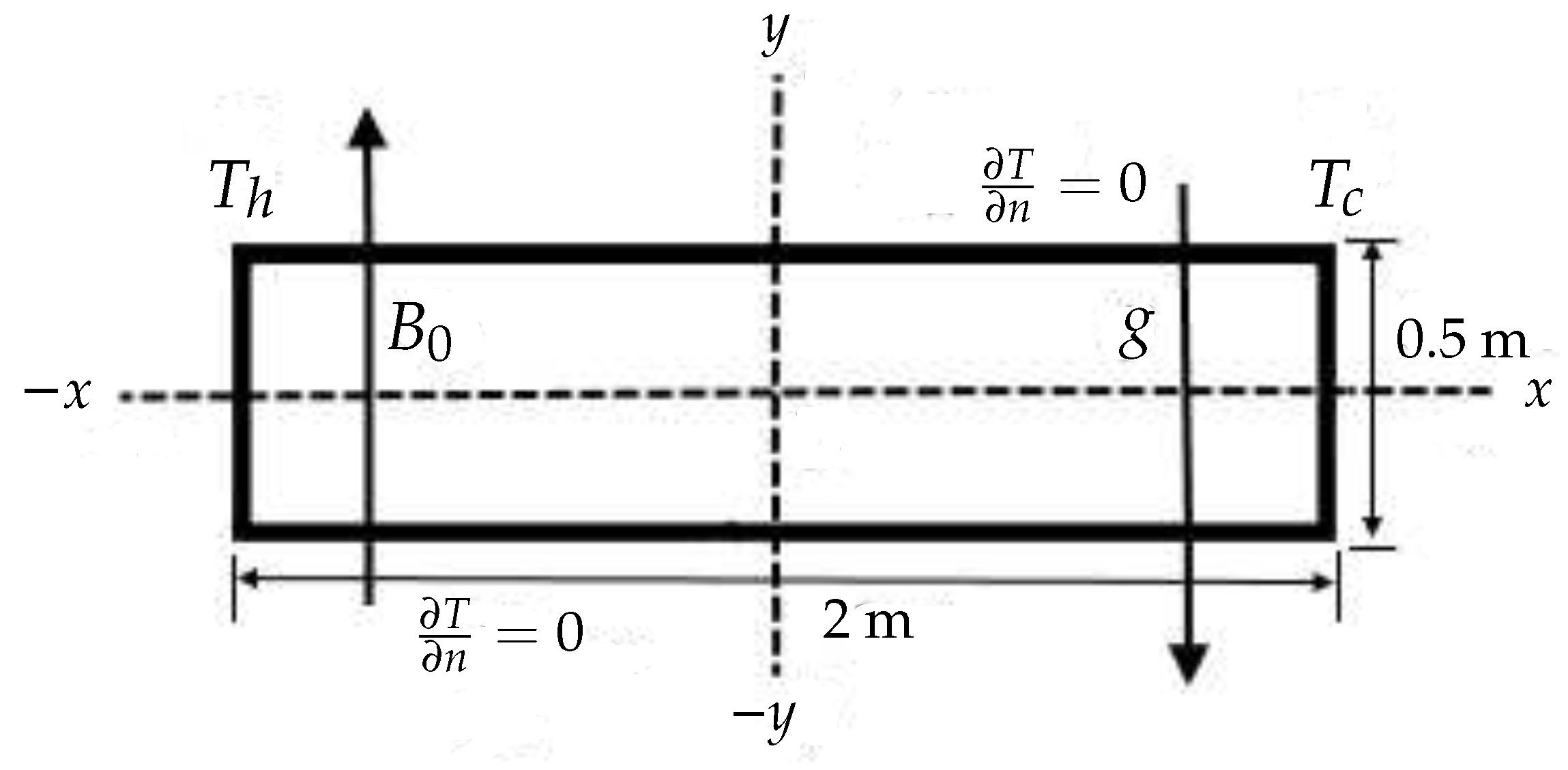
3.3. Two-Dimensional Buoyancy-Driven Flow Problem

We consider the case of buoyancy-driven flow inside a rectangular cavity with an aspect ratio of H / L = 0.25 . The schematic for this problem is shown in Figure 6.
The vertical walls are at constant temperature T h and T c , whereas the horizontal walls are thermally insulated. The magnetic field B 0 acts along the y-direction. The analytical solution for the non-dimensional velocity along the x-direction along the center vertical plane is [35,36]
U = sinh ( Ha y ) 2 sinh ( Ha / 2 ) y ,
where
U = Ha 2 G r u x H ν , Gr = g β ν 2 ( Δ T ) H 4 L , Ha = σ e μ B 0 H .
The flow properties used for this problem are T h = 30   ° C , T c = 10   ° C , C v = 10 J / kg - K , μ = 10 3 kg / m - s , k f = 1 W / m - K , β = 207 × 10 6 K 1 , ρ = 998.2 kg / m 3 , μ r = 7.9577 × 10 3 , σ e = 10 ( Ω - m ) 1 , and g = 1.552083478 × 10 4 m / s 2 , which correspond to P r = 0.01 , Gr = 2 × 10 4 , and Ha = 1000 ( B 0 = 20 Tesla). Lower Hartmann numbers are simulated using a corresponding lower value for B 0 .
The mesh specifications for the different Hartmann numbers considered are given in Table 2.
Figure 7 presents a comparison between the analytical and numerical results for a large range of Ha values (1–1000). Eswaran et al. [28] used a graded mesh with 25,351 nodes for Ha = 10 , whereas, in the present case, we use a coarse uniform mesh with 3321 nodes to obtain a solution that is in very good agreement with the analytical solution. Figure 8 and Figure 9 present, respectively, the isotherms and streamlines for Ha = 1 , Ha = 10 , and Ha = 100 .

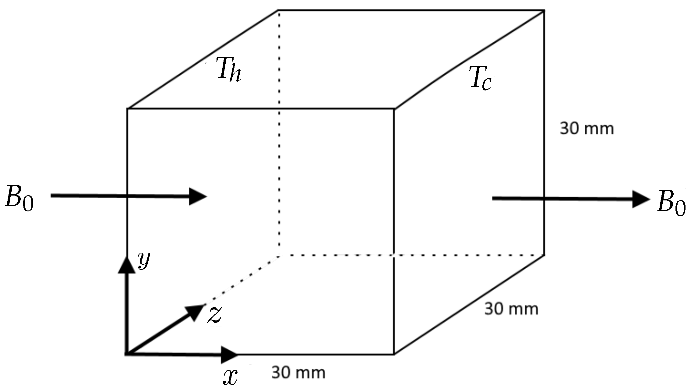
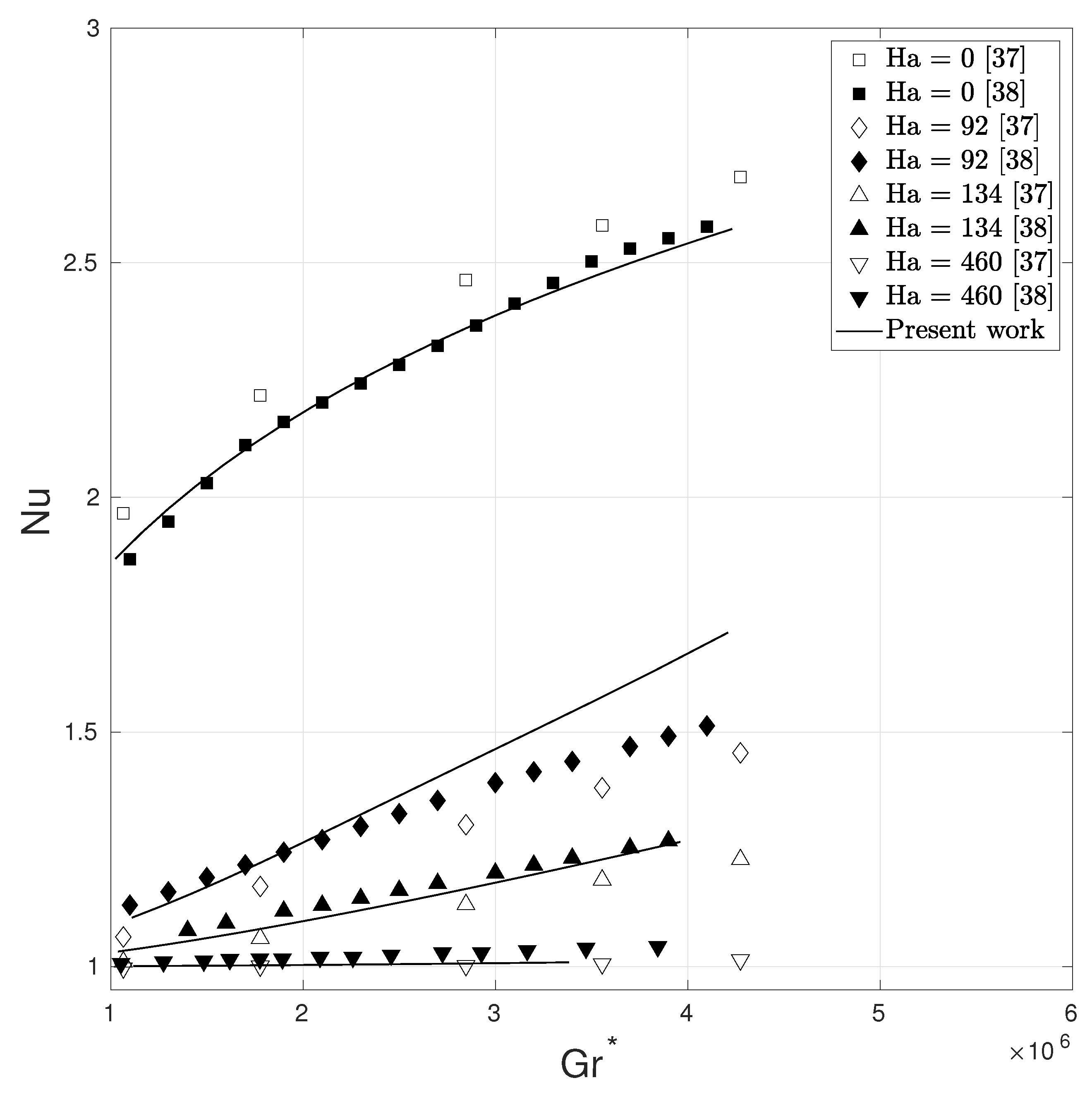
3.4. 3D Natural Convection Problem in the Presence of a Magnetic Field

This problem is based on experiments performed by Okada et al. [37]. Gallium as a working substance is kept in a 30 mm × 30 mm × 30 mm cubical cavity. A temperature difference ( T h T c ) is applied across the fluid, and a magnetic field B 0 is applied in a direction parallel to the temperature difference as shown in Figure 10.
The flow parameters used are T h = 308.15 K , T c = 278.15 K , μ = 10 3 kg / m - s , ν = 10 6 m 2 / s , β = 207 × 10 6 K 1 , C v = 756 J / kg - K , κ f = 31.5 W / m 2 - K , μ r = 7.9577 × 10 3 , σ e = 3.85 × 10 6 ( Ω - m ) 1 , Pr = 0.024 . The values of g and B 0 for different values of Ha are given in Table 3, where
Gr = g β ( T h T c ) D 3 ν 2 , Gr * = g β ν 2 κ f Q net D 4 A , Ha = σ e μ B 0 D , Nu = Q net D A κ f ( T h T c ) , B 0 = μ m H x , μ m = μ r μ 0 , μ 0 = 4 π × 10 7 .
Q net is the net rate of heat transfer ( W ) , D is the side of the cube ( 30 mm ) , and A is the cross-sectional area ( 900 mm 2 ) . The values are chosen such that the modified Grashoff number Gr * varies from 10 6 to 4.24 × 10 6 for different Ha as in [37]. Meng et al. [38] have solved this problem numerically for buoyant MHD flows at high Ha.
We use a graded mesh of 23,273 nodes and 2592 27-noded hexahedral elements for all Ha values to demonstrate the good coarse-mesh accuracy of the present formulation. Figure 11 shows a very good agreement for the Nusselt number at various Gr * and Ha.

4. Discussion

An appropriate choice of the interpolation functions for the various field variables is critical in ensuring the stability of the resulting numerical scheme. The weak implementation of the state equation used in this work ensures that a lower order interpolation can be used for the pressure, density, and temperature fields compared to the interpolation for the velocity and magnetic fields. The resulting strategy yields stable solutions for all of the field variables without the need for any stabilizing terms in the formulation, or without the need to adjust any parameters, even with coarse meshes. The monolithic nature of the strategy and the exact linearization of the variational formulation ensure a faster rate of convergence compared to a staggered approach.
Based on the numerical solutions presented, it can be said that the present formulation shows a very good coarse-mesh accuracy, and is robust and efficient even at very high Hartmann numbers.

Author Contributions

Conceptualization, C.S.J.; methodology, A.G. and C.S.J.; software, A.G.; writing—original draft preparation, A.G.; writing—review and editing, C.S.J. All authors have read and agreed to the published version of the manuscript.

Funding

This research received no external funding.

Data Availability Statement

The data that support the findings of this study are available from the corresponding author upon reasonable request.

Conflicts of Interest

The authors declare no conflict of interest.

References

  1. Shadid, J.N.; Pawlowski, R.P.; Banks, J.W.; Chacón, L.; Lin, P.T.; Tuminaro, R.S. Towards a scalable fully implicit fully coupled resistive MHD formulation with stabilized FE methods. J. Comput. Phys. 2010, 229, 7649–7671. [Google Scholar] [CrossRef] [Green Version]
  2. Guermond, J.L.; Léorat, J.; Nore, C. A new finite element method for magneto-dynamical problems: Two-dimensional results. Eur. J. Mech. B Fluids 2003, 22, 555–579. [Google Scholar] [CrossRef]
  3. Boffi, D.; Brezzi, F.; Fortin, M. Mixed Finite Elements and Applications; Springer: Berlin/Heidelberg, Germany, 2013. [Google Scholar] [CrossRef]
  4. Nesliturk, A.I.; Tezer-Sezgin, M. Finite element method solution of electrically driven magnetohydrodynamic flow. J. Comput. Appl. Math. 2006, 192, 339–352. [Google Scholar] [CrossRef] [Green Version]
  5. Salah, N.B.; Soulaimani, A.; Habashi, W.G.; Fortin, M. A conservative stabilized finite element method for magneto-hydrodynamics. Int. J. Numer. Methods Fluids 1999, 29, 535–554. [Google Scholar] [CrossRef]
  6. Salah, N.B. A Finite Element Method for the Fully Coupled Magneto-Hydrodynamics. Ph.D. Thesis, Concordia University, Montreal, QC, Canada, 1999. [Google Scholar]
  7. Codina, R.; Silva, N.H. Stabilized finite element approximation of the stationary magneto-hydrodynamics equations. Comput. Mech. 2006, 38, 344–355. [Google Scholar] [CrossRef]
  8. Gerbeau, J.F. A stabilized finite element method for the incompressible magnetohydrodynamic equations. Numer. Math. 2000, 87, 83–111. [Google Scholar] [CrossRef]
  9. Schotzau, D. Mixed finite element methods for stationary incompressible magneto–hydrodynamics. Numer. Math 2004, 96, 771–800. [Google Scholar] [CrossRef]
  10. Zhang, G.; He, Y.; Yang, D. Analysis of coupling iterations based on the finite element method for stationary magnetohydrodynamics on a general domain. Comput. Math. Appl. 2014, 68, 770–788. [Google Scholar] [CrossRef]
  11. Greif, C.; Li, D.; Schötzau, D. Wei, X. A mixed finite element method with exactly divergence-free velocities for incompressible magnetohydrodynamics. Comput. Methods Appl. Mech. Eng. 2010, 199, 2840–2855. [Google Scholar] [CrossRef]
  12. Jin, D.; Ledger, P.D.; Gil, A.J. An hp-fem framework for the simulation of electrostrictive and magnetostrictive materials Comput. Struct. 2014, 133, 131–148. [Google Scholar] [CrossRef]
  13. Ali, M.M.; Alim, M.A.; Akhter, R.; Ahmed, S.S. MHD Natural Convection Flow of CuO/Water Nanofluid in a Differentially Heated Hexagonal Enclosure with a Tilted Square Block. Int. J. Appl. Comput. Math. 2017, 3, 1047–1069. [Google Scholar] [CrossRef]
  14. Sheikholeslami, M; Zeeshan, A. Analysis of flow and heat transfer in water based nanofluid due to magnetic field in a porous enclosure with constant heat flux using CVFEM. Comput. Methods Appl. Mech. Eng. 2017, 320, 68–81. [Google Scholar] [CrossRef]
  15. Sheikholeslami, M.; Bandpy, M.G.; Ellahi, R.; Hassan, M.; Soleimani, S. Effects of MHD on Cu–water nanofluid flow and heat transfer by means of CVFEM. J. Magn. Magn. Mater. 2014, 349, 188–200. [Google Scholar] [CrossRef]
  16. Ali, B.; Rasool, G.; Hussain, S.; Baleanu, D.; Bano, S. Finite Element Study of Magnetohydrodynamics (MHD) and Activation Energy in Darcy–Forchheimer Rotating Flow of Casson Carreau Nanofluid. Processes 2020, 8, 1185. [Google Scholar] [CrossRef]
  17. Kefayati, G.H.R. Simulation of heat transfer and entropy generation of MHD natural convection of non-Newtonian nanofluid in an enclosure. Int. J. Heat Mass Transf. 2016, 92, 1066–1089. [Google Scholar] [CrossRef]
  18. Koriko, O.K.; Shah, N.A.; Saleem, S.; Chung, J.D.; Omowaye, A.J.; Oreyeni, T. Exploration of bioconvection flow of MHD thixotropic nanofluid past a vertical surface coexisting with both nanoparticles and gyrotactic microorganisms. Sci. Rep. 2021, 11, 16627. [Google Scholar] [CrossRef]
  19. Tang, H.; Kefayati, G.H.R. MHD mixed convection of viscoplastic fluids in different aspect ratios of a lid-driven cavity using LBM. Int. J. Heat Mass Transf. 2018, 124, 344–367. [Google Scholar] [CrossRef]
  20. Kefayati, G.H.R. Mesoscopic simulation of magnetic field effect on natural convection of power-law fluids in a partially heated cavity. Chem. Eng. Res. Des. 2015, 94, 337–354. [Google Scholar] [CrossRef]
  21. Kefayati, G.H.R. Simulation of vertical and horizontal magnetic fields effects on non-Newtonian power-law fluids in an internal flow using FDLBM. Comput Fluids 2015, 114, 12–25. [Google Scholar] [CrossRef]
  22. Kefayati, G.H.R. Mesoscopic simulation of magnetic field effect on Bingham fluid in an internal flow. J. Taiwan Inst. Chem. Eng. 2015, 54, 1–10. [Google Scholar] [CrossRef]
  23. Ali, A.; Awais, M.; Al-Zubaidi, A.; Saleem, S.; Khan Marwat, D.N. Hartmann boundary layer in peristaltic flow for viscoelastic fluid: Existence. Ain. Shams. Eng. J. 2021, 2090–4479. [Google Scholar] [CrossRef]
  24. Zhang, W.; Habashi, W.G.; Baruzzi, G.S.; Salah, N.B. Edge-Based Finite Element Formulation of Magnetohydrodynamics at High Mach Numbers. Int. J. Comut. Fluid Dyn. 2021, 35, 349–372. [Google Scholar] [CrossRef]
  25. Kirk, B.S.; Stogner, R.; Oliver, T.A.; Bauman, B.T. Modeling Hypersonic Entry with the Fully-Implicit Navier–Stokes (FIN-S) Stabilized Finite Element Flow Solver. Comput. Fluids 2014, 92, 281–292. [Google Scholar] [CrossRef]
  26. Ciucă, C.; Fernandez, P.; Christophe, A.L.; Nguyen, N.C.; Peraire, J.A. Implicit Hybridized Discontinuous Galerkin Methods for Compressible Magnetohydrodynamics. J. Comput. Phys. 2020, 5, 100042. [Google Scholar] [CrossRef]
  27. Llambay, P.B.; Masset, F.S. FARGO3D: A new GPU-oriented MHD code. AAS 2016, 223, 1–11. [Google Scholar]
  28. Gajbhiye, N.; Throvagunta, P.; Eswaran, V. Validation and verification of a robust 3-D MHD code. Fusion Eng. Des. 2018, 128, 7–22. [Google Scholar] [CrossRef]
  29. Nandy, A.; Jog, C.S. A monolithic finite element formulation for magnetohydrodynamics. Sadhana Indian Acad. Sci. 2018, 43, 151. [Google Scholar] [CrossRef] [Green Version]
  30. Griffiths, D.J. Introduction to Electrodynamics, 4th ed.; Cambridge University Press: Cambridge, UK, 2017; pp. 154–196. [Google Scholar]
  31. Jog, C.S. Fluid Mechanics: Foundations and Applications of Mechanics, 3rd ed.; Cambridge University Press: Cambridge, UK, 2015. [Google Scholar] [CrossRef]
  32. Bittencourt, J.A. Fundamentals of Plasma Physics, 3rd ed.; Springer: New York, NY, USA, 2004; pp. 224–226. [Google Scholar]
  33. Moreau, R. Magnetohydrodynamics; Springer: Dordrecht, The Netherlands, 1990. [Google Scholar]
  34. Dutta, S.; Jog, C.S. A monolithic arbitrary Lagrangian–Eulerian-based finite element strategy for fluid–structure interaction problems involving a compressible fluid. Int. J. Numer. Methods Eng. 2021, 122, 6037–6102. [Google Scholar] [CrossRef]
  35. Garandet, J.P.; Alboussiere, T.; Moreau, R. Buoyancy driven convection in a rectangular enclosure with a transverse magnetic field. Int. J. Heat Mass Transf. 1992, 35, 741–896. [Google Scholar] [CrossRef]
  36. Sarkar, S.; Ganguly, S.; Biswas, G. Buoyancy driven convection of nanofluids in an infinitely long channel under the effect of a magnetic field. Int. J. Heat Mass Transf. 2014, 71, 328–340. [Google Scholar] [CrossRef]
  37. Okada, K.; Ozoe, H. Experimental Heat Transfer Rates of Natural Convection of Molten Gallium Suppressed Under an External Magnetic Field in Either the X, Y, or Z Direction. J. Heat Transfer. 1992, 114, 107–114. [Google Scholar] [CrossRef]
  38. Meng, Z.; Ni, M.; Jiang, J.; Zhu, Z.; Zhou, T. Code Validation for Magnetohydrodynamic Buoyant Flow at High Hartmann Number. J. Fusion Energy 2016, 35, 148–153. [Google Scholar] [CrossRef]
Figure 1. Schematic for the 2D lid-driven cavity problem.
Fluids 07 00027 g001
Figure 2. (a) Convergence of the steady-state solution with respect to mesh refinement. (b) Convergence of the transient solution with respect to mesh and timestep refinement.
Fluids 07 00027 g002
Figure 3. Variation of (a) u x and (b) u y along the mid plane x = 0.5 m .
Fluids 07 00027 g003
Figure 4. Streamlines corresponding to the steady-state solution of the 2D lid-driven cavity problem.
Fluids 07 00027 g004
Figure 5. Comparison of the numerical and analytical solutions along the mid plane x = 0.5 m for Hartman–Poiseuille flow: (a) u x (b) H x .
Fluids 07 00027 g005
Figure 6. Schematic for the two-dimensional buoyancy-driven flow problem.
Fluids 07 00027 g006
Figure 7. Comparison of the numerical and analytical solutions for the non-dimensional velocity U along the center plane x = 0 for the two-dimensional buoyancy-driven flow problem.
Fluids 07 00027 g007
Figure 8. Isotherms for the two-dimensional buoyancy-driven flow problem at Gr = 2 × 10 4 , Ra = 2 × 10 2 . (a) Ha = 1 ; (b) Ha = 10 ; (c) Ha = 100 .
Fluids 07 00027 g008
Figure 9. Streamlines for the two-dimensional buoyancy-driven flow problem at Gr = 2 × 10 4 , Ra = 2 × 10 2 . (a) Ha = 1 ; (b) Ha = 10 ; (c) Ha = 100 .
Fluids 07 00027 g009
Figure 10. Schematic for the three-dimensional natural convection problem in the presence of a magnetic field.
Fluids 07 00027 g010
Figure 11. Comparison of the numerical results with the experimental results of Okada et al. [37] and computational results of Meng et al. [38] for Nusselt number variation with Gr * at different Ha for the 3D natural convection problem.
Fluids 07 00027 g011
Table 1. Convergence of the solution with respect to mesh and timestep refinement in the 2D lid-driven cavity problem in the presence of a magnetic field.
Mesh LevelElements t Δ E steady E transient
i 20 × 20 1 s0.14780.1276
ii 40 × 40 0.5 s0.06680.0561
iii 80 × 80 0.25 s0.02240.0284
Table 2. Mesh specifications for the two-dimensional buoyancy-driven flow problem.
HaNo. of ElementsNo. of NodesNo. of Degrees of Freedom
1 40 × 20 332115,101
10 40 × 20 332115,101
100 100 × 75 30,351142,176
1000 200 × 200 160,801759,201
Table 3. Properties used for different Ha in the 3D natural convection problem.
Ha B 0 (Tesla) g ( m / s 2 )
009.81
920.04942380820
1340.07413571320
4600.24711904220
Publisher’s Note: MDPI stays neutral with regard to jurisdictional claims in published maps and institutional affiliations.

