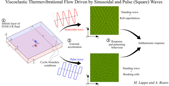
Viscoelastic Thermovibrational Flow Driven by Sinusoidal and Pulse (Square) Waves

Abstract

The present study aims to probe the role of an influential factor heretofore scarcely considered in earlier studies in the field of thermovibrational convection, that is, the specific time-varying shape of the forcing used to produce fluid motion under the effect of an imposed temperature gradient. Towards this end, two different temporal profiles of acceleration are considered: a classical (sinusoidal) and a pulse (square) wave. Their effects are analyzed in conjunction with the ability of a specific category of fluids to accumulate and release elastic energy, i.e., that of Chilcott–Rallison finitely extensible nonlinear elastic (FENE-CR) liquids. Through solution of the related governing equations in time-dependent, three-dimensional, and nonlinear form for a representative set of parameters (generalized Prandtl number $P{r}_g=8$, normalized frequency $\Omega =25$, solvent-to-total viscosity ratio $\xi =0.5$, elasticity number $\vartheta =0.1$, and vibrational Rayleigh number $R{a}_{\omega }=4000$), it is shown that while the system responds to a sinusoidal acceleration in a way that is reminiscent of modulated Rayleigh–Bénard (RB) convection in a Newtonian fluid (i.e., producing a superlattice), with a pulse wave acceleration, the flow displays a peculiar breaking-roll mode of convection that is in between classical (un-modulated) RB in viscoelastic fluids and purely thermovibrational flows. Besides these differences, these cases share important properties, namely, a temporal subharmonic response and the tendency to produce spatially standing waves.

1. Introduction

Thermally driven flows represent a vast category of phenomena with extensive background applications in various technological realms and industrial areas. In nature (where they are omnipresent), such processes are typically driven by density differences, which, in turn, are due to gradients of temperature. An increase in temperature typically makes a fluid lighter; as a result, in a steady gravitational field, relatively warm parcels of fluid tend to rise, whereas cold ones sink. Thermally driven fluid motion, however, is not an exclusive prerogative of steady acceleration fields. Time-varying (with variable sign and/or direction) body forces can indeed support similar density-driven mechanisms and excite other fascinating forms of thermal convection [1,2].

Such apparently innocuous observation is indeed at the basis of a well-known dichotomy in the literature, that is, the distinction between the classical fluid motion of thermogravitational nature and the so-called “thermovibrational” convection. The latter is called in this way as the simplest approach to have a fluid undergoing an acceleration that changes continuously sign in time is to “shake” the system containing the fluid itself. Constant amplitude “vibrations” with a given frequency result in a constant amplitude acceleration that varies in time with the same frequency of the parent vibrations and has localized minima and maxima of equal strength (absolute value). In other words, constant amplitude vibrations can produce an acceleration signal that displays no mean value (i.e., the related time-averaged value over a period of the vibrations is zero [3]).

Fluid motion induced by constant-amplitude vibrations may be regarded as the natural counterpart of buoyancy flow produced by steady gravity (see, e.g., in [4]). In fact, over the years this realization has led to the development of two branches of investigation running in parallel in the literature. These have shown that both variants are extremely sensitive to the relative inclination of the (steady or oscillatory) acceleration and the dominant temperature gradient. If they are parallel (e.g., concurrent gravity and temperature gradient), fluid motion requires that a threshold is exceeded in terms of a proper characteristic number (the so-called Rayleigh number). If they are not parallel (a special case being the condition in which they are perfectly perpendicular), then fluid motion is enabled regardless of the “position” of the considered case in the space of parameters (see, e.g., in [5] and references therein).

In the present study, we will concentrate on the first paradigm, i.e., the angle between acceleration and temperature gradient being exactly zero.

In these circumstances, when the acceleration is constant in time, the spatio-temporal behavior of the flow, which emerges from an initially quiescent state as the control parameter is increased, strongly depends on the nature of the considered fluid. For Newtonian fluids (where the only stresses present in the fluid are of a purely frictional nature), convection typically emerges in the form of steady parallel rolls. Time dependence is typically excited through a secondary bifurcation of the Hopf type (this concept being connected to the existence of well-defined instability regions in the space of parameters, e.g., the Busse balloon for the infinite layer case [6,7,8,9,10,11]). For viscoelastic fluids (special liquids where the existence of stresses that have an elastic nature is also permitted), the primary flow is intrinsically oscillatory (i.e., the first bifurcation is a Hopf bifurcation) if the elasticity of the fluid is sufficiently high; in turn, this behavior can be immediately put in relation with the well-known notion of “overstability”, i.e., the process by which the critical threshold is significantly lowered with respect to the equivalent Newtonian case [12,13,14,15,16,17,18,19,20].

Unlike thermogravitational fluid motion, however, the thermovibrational convection being considered in the present work is oscillatory by definition. Using a phenomenological perspective, the emerging flow may be seen as the combination of a “linear response” (fluid velocity and temperature oscillating with the same frequency of the forcing) and a nonlinear contribution. The properties of the latter are essentially determined by the equations governing the dynamics, which are intrinsically nonlinear per se (the nonlinearity residing essentially in the convective terms of the momentum and energy equations for standard Newtonian fluids, additional nonlinearity being brought in by the additional equations for the elastic stresses for the viscoelastic fluids). In general, the nonlinear contribution consists of various harmonics (oscillatory modes with frequencies that are integer multiples of the forcing one) and a “stationary” component, i.e., a value obtained by time-averaging the fluid velocity (or temperature) over the period of the forcing, which is not zero. Various studies conducted under the assumption of Newtonian fluid have shown that the relative importance of the linear (fluctuating) response and the time-averaged contribution depends essentially on the amplitude of the vibrations and their frequency; the aforementioned mean value typically becomes significant as the frequency grows if the amplitude of vibrations is small (this resulting in the so-called Gershuni’s regime of fluid motion [3,21,22,23,24,25,26,27]).

Vice versa, the fluctuating component is dominant if relatively small frequencies are considered [28,29]. Investigations carried out for viscoelastic fluids in this condition have led to the conclusion that the concept of overstability is still applicable [30]. Moreover, it has been shown that in terms of spatio-temporal behavior, three-dimensional (3D) standing waves are the preferred outcome for these fluids (i.e., mechanisms of convection where localized plumes periodically invert their sense of motion, giving rise to extremely ordered lattice-like patterns [30]).

The equivalent 3D studies conducted for thermogravitational flows in viscoelastic liquids have revealed quite different dynamics where elongated rolls are still possible. It has been found that the parallel convective structures typical of steady Rayleigh–Bénard (RB) convection are replaced by a peculiar mechanism of oscillations where rolls continuously break and reform in time with a new orientation in space (which is essentially perpendicular to the original one [31,32]).

In such a context, the present study aims to probe the role of an influential factor that before now has been scarcely considered, that is, the specific (temporal) shape of the forcing used to produce thermovibrational convection. All the studies cited in this introduction were indeed obtained assuming for the forcing a canonical waveform, that is, a classical sinusoidal acceleration signal. The main objective of the present numerical investigation is the assessment of the modifications induced in the patterning behavior of a viscoelastic fluid when classical sinusoidal vibrations are replaced with a “square wave”. This can be seen as a non-sinusoidal (yet periodic) forcing where the amplitude alternates (yet at a constant frequency) between fixed minimum and maximum values, with the same duration at minimum and maximum and instantaneous transitions between such extrema (also known as pulse waves). Such a change in the waveform is expected to have a remarkable impact on the dynamics of viscoelastic fluids given the ability of these liquids to accumulate and release energy according to intrinsic temporal scales [30].

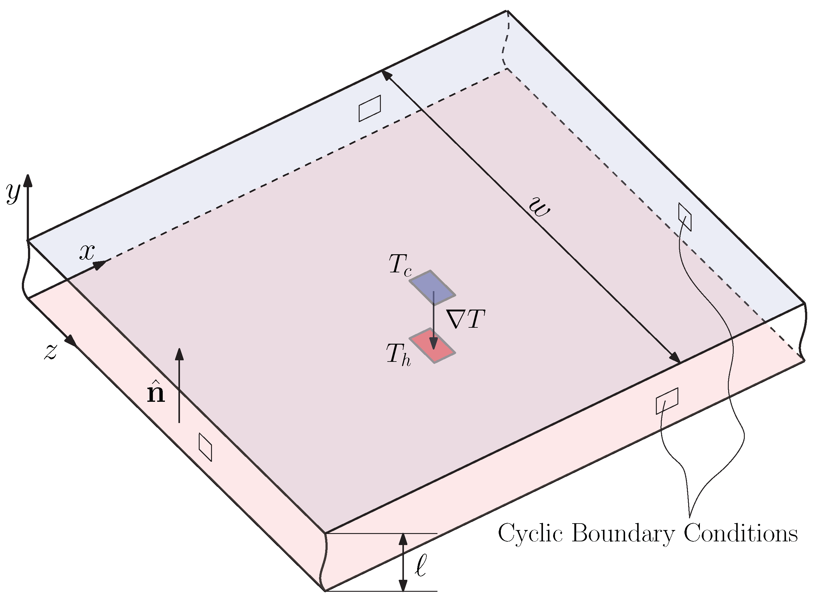
2. Mathematical Model

Following the same rationale underpinning [30], a shallow infinite layer of aspect ratio $AR=w/\ell =15$ is considered, where w represents the extension in the x and z directions (square basis), and ℓ accounts for the depth of the layer. To mimic an infinite domain, cyclic (periodic) boundary conditions are applied along the sides of the layer, while no slip walls play the role of top and bottom boundaries. Such solid walls are differentially heated in such a way that a temperature gradient is established within the liquid. The related difference of temperature reads $\Delta T=T_h-T_c$, where the subscripts h and c denote the “hot” and “cold” sides, respectively. A scheme of the domain is depicted in Figure 1.

Proper casting of the balance equations in compact form requires a model is introduced for the buoyancy force. In this regard (although in this case the acceleration acting in the system is not steady), the Oberbeck–Boussinesq approximation can still be considered valid. This must be associated with an acceleration that is an harmonic function of time, namely, $\mathbf{H}\left(t^{*}\right)$ (the symbol ${}^{*}$ indicates that the quantity is dimensional). This function depends on the “type” of the vibrations that are exciting the system. The classical way to model harmonic vibrations for thermovibrational flows (see, e.g., in [1,3,4,5,29]) is to consider a sinusoidal displacement $\mathbf{s}\left(t^{*}\right)=bsin\left(\omega t^{*}\right)\widehat{\mathbf{n}}$, where b is the amplitude, $\omega$ is the angular frequency ($\omega =2\pi f$), $\widehat{\mathbf{n}}$ is the direction of the vibrations. In such a case, taking the second derivative of $\mathbf{s}\left(t^{*}\right)$ yields

$$\mathbf{H}\left(t^{*}\right)=\gamma sin\left(\omega t^{*}\right)$$

(1)

where $\gamma =-b{\omega }^2\widehat{\mathbf{n}}$ represents the amplitude of the acceleration itself.

It is straightforward to observe that, if in place of a sinusoidal acceleration, another type of forcing is needed, the sin function in Equation (1) must be replaced with the desired waveform. For the case of a pulse (square) wave, this reads [33]

$$\mathbf{H}\left(t^{*}\right)=\gamma tanh(10sin\left(\omega t^{*}\right))$$

(2)

For the sake of simplicity, hereafter the generic harmonic acceleration will be referred to as $\mathbf{H}\left(t^{*}\right)=\gamma h\left(t^{*}\right)$.

As explained to a certain extent in the introduction, the considered fluid is assumed to be viscoelastic. In line with our preceding work [5,31], this property is modeled in the framework of the so-called finitely extensible nonlinear elastic model in Chilcott–Rallison form, generally known as FENE–CR [34,35]. This specific paradigm stems from the idea that a viscoelastic fluid can be seen as a mixture of a Newtonian solvent (having dynamic viscosity ${\eta }_s$) and a polymer solute (having dynamic viscosity ${\eta }_p$) with molecules roughly behaving as couples of beads inter-linked by a spring (dumbbell model). The resulting viscoelastic fluid has a total viscosity ${\eta }_0={\eta }_s+{\eta }_p$. It is common practice to define two mutually dependent dimensionless numbers related to the viscosity, i.e., the solvent-to-total viscosity ratio $\xi ={\eta }_s/{\eta }_0$ and the viscosity ratio $\zeta ={\eta }_p/{\eta }_s=(1-\xi )/\xi$.

This specific model allows to couple the extra viscoelastic stress tensor ${\tilde{\tau }}^{*}$ with the momentum equation. This new quantity is evaluated with a new transport equation.

To summarize, in the frame of this approach, the fluid behavior is governed by the continuity, momentum, energy, and viscoelastic stress tensor balance equations, which in dimensional form read as follows:

$$\nabla ·{\mathbf{u}}^{*}=0$$

(3)

$$\rho {\displaystyle \frac{\partial {\mathbf{u}}^{*}}{\partial t^{*}}}+\rho \nabla ·\left({\mathbf{u}}^{*}{\mathbf{u}}^{*}\right)=-\nabla p^{*}+{\eta }_s{\nabla }^2{\mathbf{u}}^{*}+\nabla ·{\tilde{\tau }}^{*}+\rho {\beta }_T\left(T-T_{\mathrm{ref}}\right)\mathbf{H}\left(t^{*}\right)$$

(4)

$${\displaystyle \frac{\partial T^{*}}{\partial t^{*}}}=-\nabla ·\left({\mathbf{u}}^{*}{T}^{*}\right)+\alpha {\nabla }^2{T}^{*}$$

(5)

$$\begin{array}{ccc}\hfill \lambda \left(\frac{\partial {\tilde{\tau }}^{*}}{\partial t^{*}}+{\mathbf{u}}^{*}·\nabla {\tilde{\tau }}^{*}\right)+f(tr\left({\tilde{\tau }}^{*}\right)){\tilde{\tau }}^{*}& =& {\eta }_{p}f(tr\left({\tilde{\tau }}^{*}\right))\left(\nabla {\mathbf{u}}^{*}+{(\nabla {\mathbf{u}}^{*})}^{⊺}\right)\hfill \\ & +& \lambda \left({\tilde{\tau }}^{*}·\nabla {\mathbf{u}}^{*}+{(\nabla {\mathbf{u}}^{*})}^{⊺}·{\tilde{\tau }}^{*}\right)\hfill \end{array}$$

(6)

where $t^{*}$ is the time, ${\mathbf{u}}^{*}$ is the velocity, $T^{*}$ is the temperature, $p^{*}$ is the pressure, $\rho$ is the density of the fluid, ${\beta }_T$ is the thermal expansion coefficient, $\alpha$ is the thermal diffusivity, and $\lambda$ is the so-called relaxation time. The function $f(tr\left({\tilde{\tau }}^{*}\right))$ is a quantity related to the possible deformation of the polymeric molecule, which in the FENE–CR is limited and modelled through the the so-called finite extensibility parameter ($L^2$); it reads

$$f(tr\left({\tilde{\tau }}^{*}\right))={\displaystyle \frac{L^2+{\displaystyle \frac{\lambda }{{\eta }_p}}tr\left({\tilde{\tau }}^{*}\right)}{L^2-3}}$$

(7)

The balance equations can then be nondimensionalized using ℓ, $\alpha /\ell$, ${\ell }^2/\alpha$, $\alpha /{\ell }^2$, $\rho {\alpha }^2/{\ell }^2$, $\Delta T$, and $\rho {\nu }_s\alpha /{\ell }^2$ (where ${\nu }_s={\eta }_s/\rho$) as scaling factors for the length, velocity, time, frequency, pressure, temperature, and extra-stress tensor, respectively. This operation generates the non-dimensional groups that fully characterize the problem under consideration, namely, the Prandtl number for the Newtonian solvent $Pr={\nu }_s/\alpha$, a generalized version of this parameter for the viscoelastic fluid $P{r}_g=Pr/\xi$, the non-dimensional frequency $\Omega ={\ell }^2\omega /\alpha$, the elasticity number $\vartheta =\lambda \alpha /{\ell }^2$, $\xi$ and $\zeta$ (both previously defined), and the vibrational Rayleigh number:

$$R{a}_{\omega }={\displaystyle \frac{b{\omega }^2{\beta }_T\Delta T{\ell }^3}{{\nu }_0\alpha }}$$

(8)

where ${\nu }_0={\eta }_0/\rho$ is the total kinematic viscosity. The balance equations in their dimensionless form therefore can be cast in condensed form as

$$\nabla ·\mathbf{u}=0$$

(9)

$${\displaystyle \frac{\partial \mathbf{u}}{\partial t}}=-\nabla p-\nabla ·\left(\mathbf{u}\mathbf{u}\right)+Pr{\nabla }^2\mathbf{u}+Pr\nabla ·\tilde{\tau }-P{r}_{g}R{a}_{\omega }Tsin(\Omega t)\widehat{\mathbf{n}}$$

(10)

$${\displaystyle \frac{\partial T}{\partial t}}=-\nabla ·\left(\mathbf{u}T\right)+{\nabla }^{2}T$$

(11)

$$\begin{array}{ccc}\hfill \vartheta \left(\frac{\partial \tilde{\tau }}{\partial t}+\mathbf{u}·\nabla \tilde{\tau }\right)+f(tr\left({\tilde{\tau }}^{*}\right))\tilde{\tau }& =& \zeta f(tr\left({\tilde{\tau }}^{*}\right))\left(\nabla \mathbf{u}+{(\nabla \mathbf{u})}^{⊺}\right)\hfill \\ & +& \vartheta \left(\tilde{\tau }·\nabla \mathbf{u}+{(\nabla \mathbf{u})}^{⊺}·\tilde{\tau }\right)\hfill \end{array}$$

(12)

3. Numerical Method

The computational platform openFOAM^® is employed here to solve numerically the set of balance equations previously defined. In particular, the related segregated time-marching procedure directly relies on the PISO (Pressure Implicit with Splitting of Operator) algorithm to couple velocity and pressure fields, and the Rie and Chow scheme [36] to avoid checkerboarding of the latter one.

The balance equations have been discretized over a uniform Cartesian grid having $200\times 35\times 200$ cells (see in [30] for the complete grid independence analysis). All the diffusive and convective terms have been evaluated though a second-order accurate central difference scheme with the exception of the convective term of Equation (12), where the Minmod scheme has been used to improve the algorithm stability. Furthermore, to mitigate the effect of possible numerical singularities, the numerical solver implements Equation (10) as [37]:

$${\displaystyle \frac{\partial \mathbf{u}}{\partial t}}+\nabla ·\left(\mathbf{u}\mathbf{u}\right)-Pr(1+\zeta ){\nabla }^2\mathbf{u}=-\nabla p-Pr\zeta {\nabla }^2\mathbf{u}+Pr\nabla ·\tilde{\tau }-P{r}_{g}R{a}_{\omega }Tsin(\Omega t)$$

(13)

As the reader will realize by comparing Equations (10) and (13), an extra diffusive term $Pr\zeta {\nabla }^2\mathbf{u}$ has been added to both sides of the momentum equation. Although the two equations are equivalent from a mathematical standpoint, in the numerical framework, the two extra diffusive terms can be integrated using different approaches (namely, one is integrated implicitly while the other one explicitly). This technique generates quantitatively negligible numerical diffusion, which, however, improves the stability and the robustness of the solver, as witnessed by earlier studies (see in [5,29,30,31,38] for further details about the code validation and its application to the case of both Newtonian and viscoelastic fluids).

4. Results

We focus on a layer of viscoelastic (FENE–CR) fluid with $P{r}_g=8$, $\xi =0.5$, and $\vartheta =0.1$ subjected to either sinusoidal or square vibrations having frequency $\Omega =25$. For both cases, the resulting vibrational Rayleigh number is $R{a}_{\omega }=4000$. Furthermore, the model parameter $L^2$ is set to 200 as in our previous studies (see in [5,31]). Let us recall that the FENE-CR can adequately represent highly elastic solutions known as “Boger fluids” (see, e.g., in [39]), able to retain an essentially constant viscosity over a wide range of shear rates. Relevant examples are represented by a class of water-based polymer dilute solutions at ambient or moderate temperatures, e.g., water between 25 ${}^{\circ }\mathrm{C}$ and 50 ${}^{\circ }\mathrm{C}$ with limited amount of a polymer such a PAM, PEG, PEO, PVP, Xanthan Gum, etc., for which the Prandtl number would be similar to that considered in the present work ($P{r}_g\cong 8$) and $\xi <1$. The rheological parameters ($P{r}_g$ and $\xi$) considered here are almost identical to those examined by Li and Khayat [39], who assumed a Boger fluid with $P{r}_g\cong 7$ (and $\xi$ varying in the range between 0 and $0.79$). Assuming $\lambda \cong {10}^{-3}$ s (a typical realistic value for small polymer concentrations) and thermal diffusivity $\alpha \cong 1.5\times {10}^{-7}$ m${}^2$/s over this range of temperatures, these values would correspond to $\vartheta =0.1$ setting $0.04$ mm as the distance between the plates.

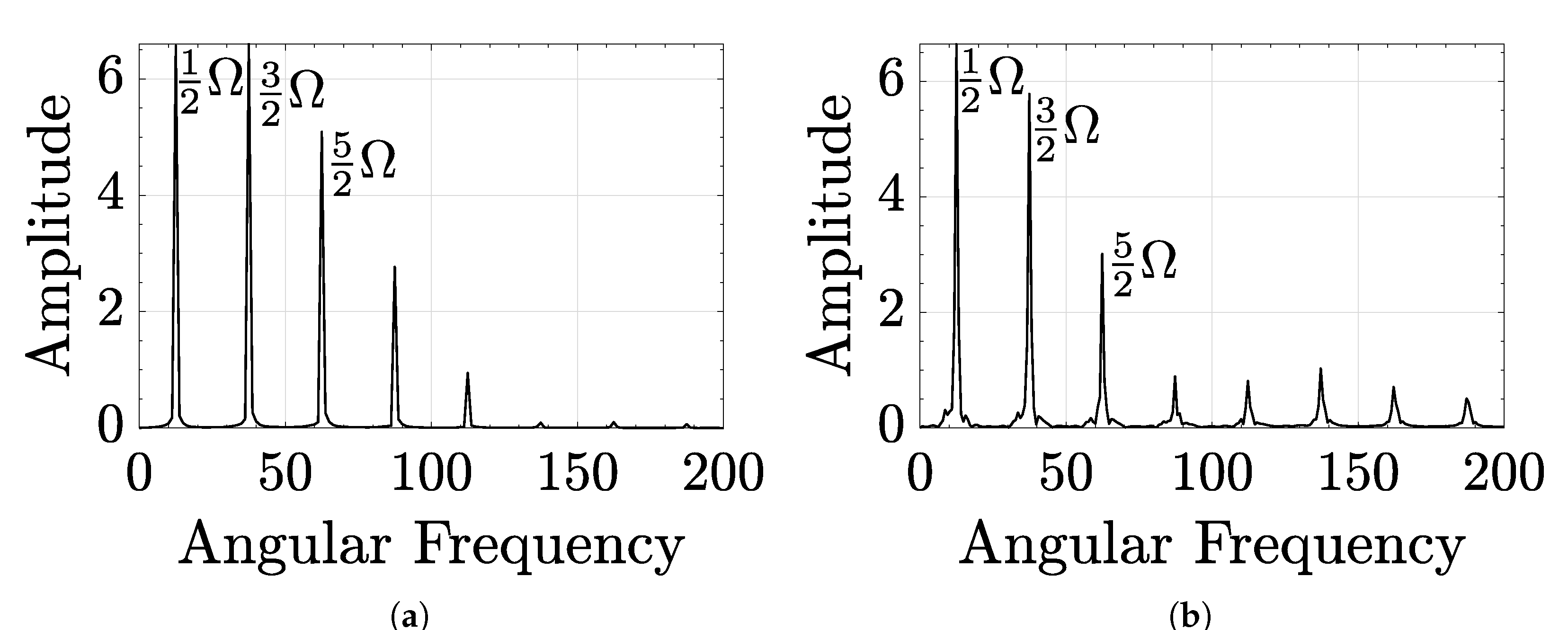
4.1. Forcing and Related System Response

Given the complexity of the considered subject, before starting to deal with the structure and evolution of the fluid dynamic field, for the convenience of the reader, in this subsection the system response is initially assessed in terms of “localized” or “global” parameters (by which drawing initial conclusions on the behavior of the system is relatively straightforward).

In particular, in order to highlight differences and similarities between the two “shapes” of the acceleration signal, we concentrate on the time evolution of two representative quantities, namely, the axial fluid velocity (the velocity component perpendicular to the solid walls) recorded by a virtual probe located in the center of the layer, i.e., (7.5, 0.5, 7.5), and an integral quantity, that is the Nusselt number calculated on the hot (bottom) plate as:

$$Nu\left(t\right)=\frac{1}{A}{\int }_A\nabla T\left(t\right)·{\mathbf{n}}_{\mathrm{plate}}dA$$

(14)

where ${\mathbf{n}}_{\mathrm{plate}}$ in the unit vector normal to the boundary, and A is the area of the heated plate.

Along these lines, Figure 2 provides the evolution in time of the two aforementioned characteristic thermal and fluid dynamic quantities together with the forcing. It can be seen that, when the external force (in red) $h\left(t\right)>0$, i.e. the acceleration has a positive direction (with respect to the unit vector $\widehat{\mathbf{n}}$, see Figure 1), the effect of the vibration is stabilizing, i.e., the vibrations act as a damper for the convective instability. By contrast, when the external force $h\left(t\right)<0$, the vibrations act in a way that is similar to the steady gravitational acceleration in the classical problem of Rayleigh–Bénard convection. Therefore, in this time interval vibrations are destabilizing, i.e., they promote convective motion. These simple arguments also clarify the reason why the Nusselt number and the forcing are out of phase. The Nusselt number is largely increased in the stage where vibrations play a destabilizing role and tends to the unit value (corresponding to quiescent conditions) as their effect is reverted.

Given this premise, it is easy to realize that, due the peculiar shape of the forcing, the switch between stabilizing and destabilizing phases can happen in different ways: the smooth transition, typical of the sinusoidal wave is taken over by an abrupt change in the acceleration direction for the case with the pulse wave. Moreover, as a result of the different shape of the forcing signal, the pulse wave might be expected to exert a stronger influence on the fluid.

In order to prove the last statement, it is worth comparing $Nu\left(t\right)$ for the two cases. As quantitatively substantiated by the data, the maximum and the time average value of the Nusselt number are lower for the case with sinusoidal acceleration ($N{u}_{\max }=1.88$, $N{u}_{\mathrm{av}}=1.18$) and bigger for the pulse one ($N{u}_{\max }=2.17$, $N{u}_{\mathrm{av}}=1.30$). A justification for this trend can be elaborated in its simplest form on the basis of the argument that while the sinusoidal acceleration attains its maximum intensity for a single instant in time, the square acceleration maintains a constant maximum intensity for half of the period of oscillations.

The axial velocity signal can also be used to get useful insights into these dynamics. Interestingly, in the stabilizing semi-period, both signals (hereafter $v_S\left(t\right)$ and $v_P\left(t\right)$ for the sinusoidal and pulse waves respectively) reach a zero value at certain time. However, a careful analysis of their shape reveals that while $v_P\left(t\right)$ is stabilized to a null value in a certain interval of the stabilizing period, $v_S\left(t\right)$ changes continuously in this interval, i.e., $d{v}_S/dt\ne 0$ in every time sub-interval (while it can locally reach 0).

In the light of these initial findings, the reader may expect that when the the fluid is excited by pulse waves, it will display a more involved behavior in the destabilizing phase if compared with the case of sinusoidal forcing for the same value of $R{a}_{\omega }$ (we will come back to this interesting concept later).

As a concluding task for this initial analysis, we also calculated the frequency of the $Nu\left(t\right)$ and $v\left(t\right)$ signals. In agreement with the earlier results by Boaro and Lappa [30] and Lyubimova and Kovalevskaya [33], obtained with a nonlinear numerical approach and linear stability analysis, respectively, the flow field exhibits a half-subharmonic response to both types of wave, i.e., the frequency of $v\left(t\right)$ is half of the frequency of the acceleration, that is $\Omega /2$ (interestingly as shown in Figure 3, the related frequency spectrum displays three dominant frequencies, namely $\Omega /2$, $\Omega +\Omega /2=3\Omega /2$ and $2\Omega +\Omega /2=5\Omega /2$, where the second and the third components are produced by the obvious nonlinear interference between the flow sub-harmonic response and the forcing). Yet in accordance with the work in [30], $Nu\left(t\right)$ shows a simple harmonic response (its frequency is exactly $\Omega$).

Before moving to the next section, taking into account the periodicity of the flow field ($\mathbf{u}\left(t_0\right)=\mathbf{u}(t_0+2T_{\Omega })$, $T_{\Omega }=2\pi /\Omega$), we conveniently define four sub-intervals of time: ${\mathcal{I}}_1=[t_0,T_{\Omega }/2]$, ${\mathcal{I}}_2=[T_{\Omega }/2,T_{\Omega }]$, ${\mathcal{I}}_3=[T_{\Omega },3/2T_{\Omega }]$, and ${\mathcal{I}}_4=[3/2T_{\Omega },2T_{\Omega }]$, where $t_0$ is a convenient instant of time. Here, we select $t_0=17.94$ for the case of sinusoidal acceleration and $t_0=11.14$ for the pulse acceleration (see Figure 2). We also take advantage of this subsection to introduce another parameter useful for the understanding of these phenomena, that is, the ratio between the relaxation time of the polymer $\lambda$ and the period of the external forcing $T_{\omega }=2\pi /\omega$ [5,30]. It is easy to verify that this parameter depends on two non-dimensional numbers defined in the preceding section and reads $\Sigma =\vartheta \Omega /2\pi$. As in our simulation both $\vartheta$ and $\Omega$ are fixed, $\Sigma =0.4$.

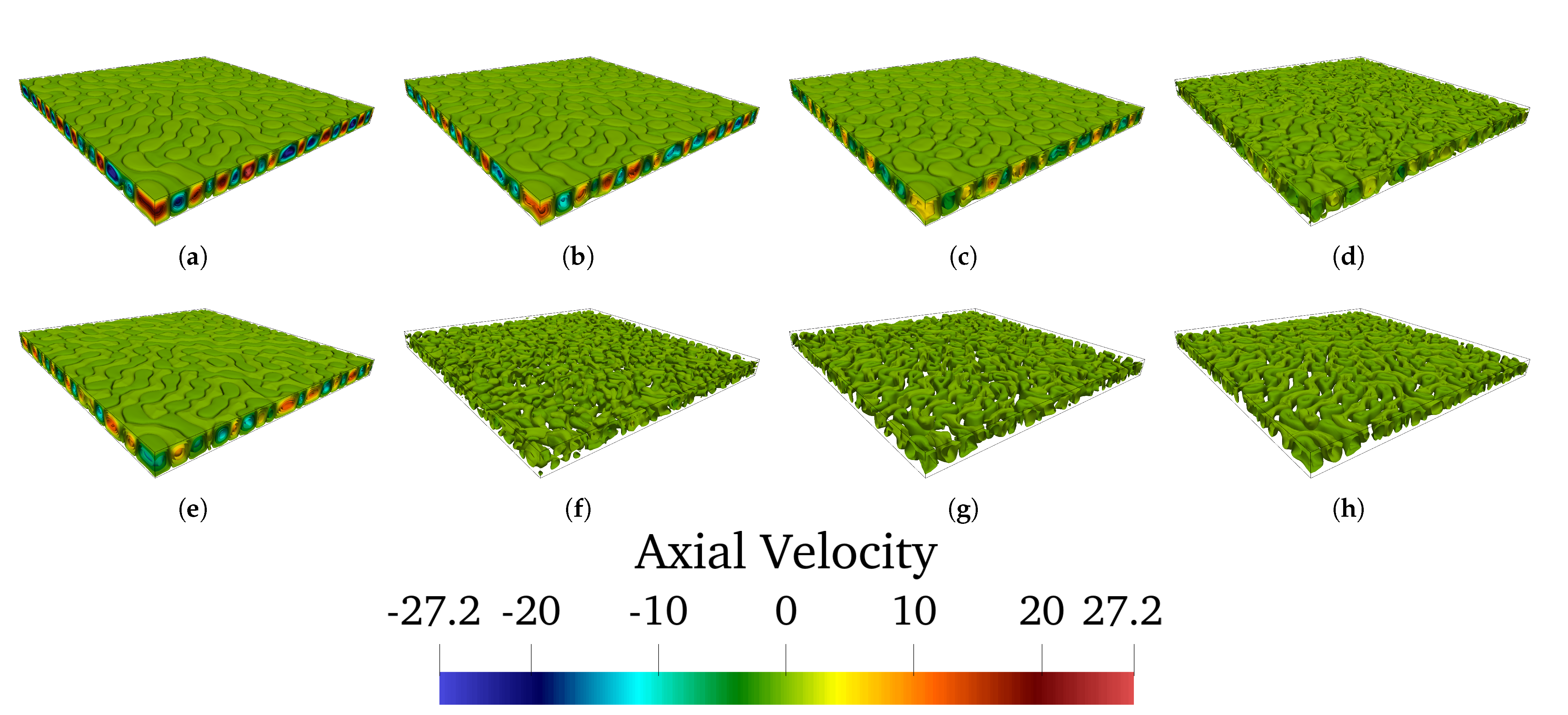
4.2. Patterning Behaviour and 3D Evolution

In this section (entirely dedicated to the analysis of the 3D behaviour of the considered flows), first we examine the 3D isosurfaces of the axial velocity for the case of sinusoidal shaking for $t\in {\mathcal{I}}_1$, see Figure 4.

At the time $t_0$ ( Figure 4a), the flow displays an ordered convective structure consisting of groups of parallel rolls each oriented along a given preferential direction. The evolution of this pattern is quite simple. As time progresses, the intensity of the axial velocity becomes smaller ( Figure 4b) until the rolls change their sense of rotation ( Figure 4c). This pulsation of the velocity field is a common solution for viscoelastic Rayleigh-Bénard systems and it is generally referred to in the literature as standing wave (see in [1] and reference therein).

Although after the inversion of the sense of rotation the intensity of the axial velocity tends to increase, it never reaches again the same value that it had at $t=t_0$ ( Figure 4d). Indeed, the acceleration is changing direction, and therefore the stabilizing effect of the vibrations starts to influence the amplitude of convection. As evident in s Figure 4e–h, interestingly, the rolls keep pulsating. However, this pulsation is no longer a result of a variation in the direction of the buoyancy force, rather it is driven by the residual elastic energy stored in the polymer molecules. This concept will be discussed afterwards.

Here, we limit ourselves to pointing out that, from a phenomenological point of view, in the initial part of the interval ${\mathcal{I}}_2$, Figure 5a, even if the acceleration is in its stabilizing phase, the intensity of the rolls increases again: the rolls, initially disperse in the domain, start to grow in intensity until they merge together ( Figure 5a–d).

It is also worth noticing that after the last inversion of sense, visible in Figure 4a–d, the rolls have not changed again their sense of rotation. However, as now the fluid motion is sustained only by the elastic energy stored in the fluid in the preceding destabilizing phase and not by the buoyancy force, the intensity of the velocity field becomes smaller as the elastic energy is dissipated through viscosity effects (compare s Figure 4d and Figure 5d).

As the flow evolves, the acceleration changes it sign and starts to play again a destabilizing role, thereby promoting the rise of the velocity field (see Figure 5f,g). Now, the buoyancy force that drives the fluid motion, along with the elastic energy, leads to a situation similar to the initial one ($t=t_0$), both for intensity and shape of the rolls, but with a different sense of rotation as evident in Figure 5h.

The second part of the oscillation period (${\mathcal{I}}_3$ and ${\mathcal{I}}_4$) evolves in similar way to the one just described, and for the sake of brevity, we do not describe it in detail.

Rather, we concentrate on the companion case, that is, the situation with the pulse acceleration (see Figure 6 for the behavior over the interval ${\mathcal{I}}_1$). Remarkably, it can be seen that the rolls are no longer aligned along a particular direction. Instead, they form randomly organized structures. The elongated shape that characterizes the case with sinusoidal vibration is now replaced by a mix between short longitudinal and rounded rolls as depicted in Figure 6a.

Recalling the concepts introduced in the earlier subsection, this scenario might be seen as a realization of the increased complexity of the flow expected when the acceleration follows a pulse wave time evolution.

Although the spatio-temporal behavior differs in the two cases under analysis, however the leading mechanism of evolution remains basically the same, namely, a standing wave. Indeed, the velocity field initially undergoes a shrinkage in intensity ( Figure 6b,c) until eventually the fluid changes its sense of rotation ( Figure 6d,e). It is worth observing that also in this case the overall intensity of the velocity field after the first inversion is smaller than that in the initial frame (compare Figure 6a–e).

Despite these similarities, however, a closer look at the first part of the pattern evolution ( Figure 6a–c) reveals that a secondary mechanism is at play in this case, namely, a breaking roll mode of convection [31,32]. This specific behavior has been already observed as a typical mode of convection in classical Rayleigh–Bénard viscoelastic flows. Its dynamics basically consists of convective rolls that break and reform but in a direction that is perpendicular to the original one. To visualize this process, as an example, the reader may consider the first roll in the corner of the layer in Figure 6a. It is easy to observe that, as the pattern evolves, this rolls tends to merge with the closest roll of the same sign ( Figure 6b,c).

Nonetheless, this peculiar mechanism is mediated by the predominant standing wave and by the fact that in the meantime the vibrations became stabilizing for the flow field (and therefore, the fluid motion is no longer driven by buoyancy but only by the elastic energy stored by the polymer molecules).

When the vibrations become stabilizing, the standing wave is still the dominant solution. In this case the fluid has stored enough energy to continue pulsating and to invert the sense of rotation two other times ( Figure 6e–g).

As the interval ${\mathcal{I}}_2$ is entered, the vibrations are more or less at half of their stabilizing phase. In this stage, the acceleration has a constant value (as opposed to a sinusoidal acceleration, which changes continuously in time). This constant stabilizing acceleration has the effect to dampen and almost annihilate the convective structures. This becomes more evident when the patterning behaviors for sinusoidal and pulse forcing are compared in ${\mathcal{I}}_2$ (compare Figure 5 and Figure 7).

As the system enters the second part of ${\mathcal{I}}_2$, the acceleration suddenly changes its direction. As a result, convective instabilities are newly excited and the velocity field starts increasing its intensity. The spatial arrangement of the rolls is the same as at the beginning of ${\mathcal{I}}_1$ but with an inversion of the sense of rotation (as depicted in Figure 7e–h).

The dynamics in ${\mathcal{I}}_3$ and in ${\mathcal{I}}_4$ are relatively similar to the one just described and for this reason we omit to report them. However, it is worth highlighting that the breaking rolls mechanism is still effective over ${\mathcal{I}}_3$.

As a concluding remark for this subsection, one last point should be clarified. As we have illustrated on the basis of a purely heuristic approach, a key factor driving the fascinating dynamics of the system under analysis is its ability to retain elastic energy and release it when the external time dependent forcing does not play a destabilizing role. A classical way to estimate the local elastic energy in a viscoelastic fluid is to calculate the trace of the extra-stress tensor $tr\left(\tilde{\tau }\right)$ (this quantity being proportional to the local elastic energy) [40].

In Figure 8, we report the evolution of $tr\left(\tilde{\tau }\right)$, hereafter we will simply call this quantity “elastic energy”, along a fixed line parallel to the x direction (belonging to the mid-height plane, i.e., $0<x<15$, $y=0.5$, and $z=7.5$) as a function of time (over the interval $2T_{\Omega }$). On this basis, it is easy to see that moving from a sinusoidal to a pulse wave acceleration increases the amount of elastic energy stored by the polymer molecules. Further, note that the elastic energy field exhibits a harmonic response to the periodic forcing, regardless of its shape (waveform).

5. Discussion and Conclusions

The results presented in this study should be regarded as an extension of previous work of the present authors on these subjects. On one hand, we have considered conditions close to those examined by Boaro and Lappa [30], i.e., thermovibrational convection in an infinite layer of viscoelastic fluid having $P{r}_g=O\left(10\right)$, and with a similar frequency of the external forcing (set as sinusoidal wave in Boaro and Lappa [30]). On the other hand, a FENE–CR fluid with $L^2=200$ having $P{r}_g=8$, $\xi =0.5$, and $\vartheta =0.1$ has been assumed (as in Lappa and Boaro [31], where attention was paid to classical Rayleigh–Bénard convection, i.e., the case with acceleration constant in time and space).

In the present work, the parameter $\Sigma$ has been fixed to $0.4$ (a value smaller than 1), which implies that in a period of vibrations, the polymer molecules are potentially able to relax and go back to their initial configuration. This is the feature allowing the system to release elastic energy when it enters the stabilizing phase of the vibrations (where such energy is progressively dissipated by viscous effects, similarly to what happens in an harmonic oscillator, see Figure 8).

As illustrated in the results section, in the case of sinusoidal forcing, the periodic excitation and dampening of convective modes (mediated by the accumulation and release of elastic energy) can generate complex-ordered structures.

Following the classification made by Rogers and coworker to categorize complex ordered structures arising from modulated Rayleigh–Bénard convection in Newtonian fluids [41,42,43,44], here, the observed patterns might be classified as roll superlattices. The roll superlattice is a subharmonic pattern emerging in states that are slightly supercritical. Once the Rayleigh number is increased and exceeds a certain threshold (which, in turn, depends on the amplitude of vibrations), these planforms can undergo a transition to a square superlattice (SQS) state [41].

Given these premises, it is interesting to compare the results of the present study ($\vartheta =0.1$), with those reported in [30] (considering in particular the cases with $\vartheta =0.06$ and $0.24$). In that work, “more” supercritical solutions were examined and the obtained superlattice-like structures were akin to the SQS observed in the modulated Rayleigh–Bénard problem. This indicates that the general conclusion that an increase in the critical parameter can turn a roll superlattice into an SQS also holds for thermovibrational convection in a viscoelastic fluid.

Moving forward to the case with pulse wave acceleration, it can be concluded that the ordered patterns seen for the sinusoidal forcing are taken over by a distribution of rolls that is more similar to the one observed in classical RB convection in viscoelastic fluids. In particular, the initial distribution of the rolls is reminiscent of the flow pattern that arises in a shallow viscoelastic liquid bridge (see [31] where the following case was considered: $A=0.17$, $Ra=2000$, $\vartheta =0.1$, where $A=\mathrm{height}/\mathrm{diameter}$ and $Ra$ represent the classical Rayleigh number). In [31], the flow was found to display a peculiar breaking-roll evolution. In the present case, this mechanism (sustained by buoyancy forces) vanishes as soon as the system enters its stabilizing phase (the differences between the two systems can obviously be found in the different cause-and-effect relationships enabled by steady and time-varying accelerations).

For the sake of completeness, we wish to report that the ability of modulation to cause a departure from the tendency of classical RB convection to produce steady parallel rolls has also been observed in Newtonian fluids where in place of mechanical forcing (vibrations), thermal forcing was implemented (in terms of time-dependent top and/or bottom temperature, see Hohenberg and Swift [45] and Meyer et al. [46]). We take those studies, where such thermal modulations were proved to cause a competition between the standard parallel rolls and hexagonal cells through a mechanism akin to that effective in non-OB (Oberbeck–Boussinesq) systems, as a cue for a possible extension of the present research.

Another exciting prospect for the future is to investigate the vibrationally modulated problem for additional (non-unit) values of the parameter $\Sigma$, for which the relaxation time of the polymer molecules is smaller or larger than the period of the forcing. This factor is also expected to contribute significantly to the number of modes that can be excited in the fluid and alter the mechanisms depicted above, thereby influencing the emerging patterns.

References

1. Lappa, M. Thermal Convection: Patterns, Evolution and Stability; John Wiley & Sons, Ltd.: Chichester, UK, 2009. [Google Scholar] [CrossRef]
2. Mialdun, A.; Ryzhkov, I.I.; Melnikov, D.E.; Shevtsova, V. Experimental Evidence of Thermal Vibrational Convection in a Nonuniformly Heated Fluid in a Reduced Gravity Environment. Phys. Rev. Lett. 2008, 101, 084501. [Google Scholar] [CrossRef] [PubMed] [Green Version]
3. Savino, R.; Lappa, M. Assessment of Thermovibrational Theory: Application to G -Jitter on the Space Station. J. Spacecr. Rocket. 2003, 40, 201–210. [Google Scholar] [CrossRef]
4. Lappa, M. Control of Convection Patterning and Intensity in Shallow Cavities by Harmonic Vibrations. Microgravity Sci. Technol. 2016, 28, 29–39. [Google Scholar] [CrossRef] [Green Version]
5. Boaro, A.; Lappa, M. Multicellular states of viscoelastic thermovibrational convection in a square cavity. Phys. Fluids 2021, 33, 033105. [Google Scholar] [CrossRef]
6. Busse, F.H.; Whitehead, J.A. Instabilities of convection rolls in a high Prandtl number fluid. J. Fluid Mech. 1971, 47, 305–320. [Google Scholar] [CrossRef] [Green Version]
7. Busse, F.H.; Clever, R.M. Instabilities of convection rolls in a fluid of moderate Prandtl number. J. Fluid Mech. 1979, 91, 319–335. [Google Scholar] [CrossRef]
8. Clever, R.M.; Busse, F.H. Nonlinear oscillatory convection. J. Fluid Mech. 1987, 176, 403–417. [Google Scholar] [CrossRef]
9. Clever, R.M.; Busse, F.H. Convection at very low Prandtl numbers. Phys. Fluids A Fluid Dyn. 1990, 2, 334–339. [Google Scholar] [CrossRef]
10. Clever, R.M.; Busse, F.H. Steady and oscillatory bimodal convection. J. Fluid Mech. 1994, 271, 103–118. [Google Scholar] [CrossRef]
11. Clever, R.M.; Busse, F.H. Standing and travelling oscillatory blob convection. J. Fluid Mech. 1995, 297, 255–273. [Google Scholar] [CrossRef]
12. Green, T. Oscillating Convection in an Elasticoviscous Liquid. Phys. Fluids 1968, 11, 1410–1412. [Google Scholar] [CrossRef]
13. Vest, C.M.; Arpaci, V.S. Overstability of a viscoelastic fluid layer heated from below. J. Fluid Mech. 1969, 36, 613–623. [Google Scholar] [CrossRef]
14. Sokolov, M.; Tanner, R.I. Convective Stability of a General Viscoelastic Fluid Heated from Below. Phys. Fluids 1972, 15, 534–539. [Google Scholar] [CrossRef]
15. Larson, R.G. Instabilities in viscoelastic flows. Rheol. Acta 1992, 31, 213–263. [Google Scholar] [CrossRef]
16. Krapivina, E.N.; Lyubimova, T.P. Nonlinear regimes of convection of an elasticoviscous fluid in a closed cavity heated from below. Fluid Dyn. 2000, 35, 473–478. [Google Scholar] [CrossRef]
17. Park, H.M.; Shin, K.S.; Sohn, H.S. Numerical simulation of thermal convection of viscoelastic fluids using the grid-by-grid inversion method. Int. J. Heat Mass Transf. 2009, 52, 4851–4861. [Google Scholar] [CrossRef]
18. Park, H.M.; Lim, J.Y. A new numerical algorithm for viscoelastic fluid flows: The grid-by-grid inversion method. J. Non-Newton. Fluid Mech. 2010, 165, 238–246. [Google Scholar] [CrossRef]
19. Kovalevskaya, K.V.; Lyubimova, T.P. Onset and nonlinear regimes of convection of an elastoviscous fluid in a closed cavity heated from below. Fluid Dyn. 2011, 46, 854–863. [Google Scholar] [CrossRef]
20. Park, H.M. Peculiarity in the Rayleigh-Bénard convection of viscoelastic fluids. Int. J. Therm. Sci. 2018, 132, 34–41. [Google Scholar] [CrossRef]
21. Simonenko, I.B.; Zen’kovskaya, S. On the effect of high frequency vibrations on the origin of convection. Izv. Akad. Nauk SSSR Ser. Mech. Zhidk. Gaza 1966, 5, 51–55. [Google Scholar]
22. Simonenko, I.B. A justification of the averaging method for a problem of convection in a field of rapidly oscillating forces and for other parabolic equations. Math. USSR-Sb. 1972, 16, 245–263. [Google Scholar] [CrossRef]
23. Gershuni, G.Z.; Zhukhovitskii, E.M. Free thermal convection in a vibrational field under conditions of weightlessness. Sov. Phys. Dokl. 1979, 24, 894–896. [Google Scholar]
24. Gershuni, G.Z.; Zhukhovitskii, E.M.; Yurkov, Y.S. Vibrational thermal convection in a rectangular cavity. Fluid Dyn. 1982, 17, 565–569. [Google Scholar] [CrossRef]
25. Gershuni, G.Z.; Zhukhovitskii, E.M. Vibrational thermal convection in zero gravity. Fluid. Mech. Sov. Res. 1986, 15, 63–84. [Google Scholar]
26. Lappa, M. Fluids, Materials and Microgravity: Numerical Techniques and Insights into the Physics, 1st ed.; Elsevier Science: Oxford, UK, 2004. [Google Scholar] [CrossRef]
27. Bouarab, S.; Mokhtari, F.; Kaddeche, S.; Henry, D.; Botton, V.; Medelfef, A. Theoretical and numerical study on high frequency vibrational convection: Influence of the vibration direction on the flow structure. Phys. Fluids 2019, 31, 043605. [Google Scholar] [CrossRef] [Green Version]
28. Hirata, K.; Sasaki, T.; Tanigawa, H. Vibrational effects on convection in a square cavity at zero gravity. J. Fluid Mech. 2001, 445, 327–344. [Google Scholar] [CrossRef]
29. Crewdson, G.; Lappa, M. The Zoo of Modes of Convection in Liquids Vibrated along the Direction of the Temperature Gradient. Fluids 2021, 6, 30. [Google Scholar] [CrossRef]
30. Boaro, A.; Lappa, M. Competition of overstability and stabilizing effects in viscoelastic thermovibrational flow. Phys. Rev. E 2021, 104, 025102. [Google Scholar] [CrossRef]
31. Lappa, M.; Boaro, A. Rayleigh–Bénard convection in viscoelastic liquid bridges. J. Fluid Mech. 2020, 904, A2. [Google Scholar] [CrossRef]
32. Lappa, M. Thermally-Driven Flows in Polymeric Liquids. In Reference Module in Materials Science and Materials Engineering; Elsevier: Amsterdam, The Netherlands, 2020. [Google Scholar]
33. Lyubimova, T.; Kovalevskaya, K. Gravity modulation effect on the onset of thermal buoyancy convection in a horizontal layer of the Oldroyd fluid. Fluid Dyn. Res. 2016, 48, 061419. [Google Scholar] [CrossRef]
34. Bird, R.B.; Dotson, P.J.; Johnson, N. Polymer solution rheology based on a finitely extensible bead—Spring chain model. J. Non-Newton. Fluid Mech. 1980, 7, 213–235. [Google Scholar] [CrossRef]
35. Chilcott, M.D.; Rallison, J.M. Creeping flow of dilute polymer solutions past cylinders and spheres. J. Non-Newton. Fluid Mech. 1988, 29, 381–432. [Google Scholar] [CrossRef]
36. Rhie, C.M.; Chow, W.L. Numerical study of the turbulent flow past an airfoil with trailing edge separation. AIAA J. 1983, 21, 1525–1532. [Google Scholar] [CrossRef]
37. Favero, J.L.; Secchi, A.R.; Cardozo, N.S.M.; Jasak, H. Viscoelastic flow analysis using the software OpenFOAM and differential constitutive equations. J. Non-Newton. Fluid Mech. 2010, 165, 1625–1636. [Google Scholar] [CrossRef]
38. Crewdson, G.; Lappa, L. Thermally-driven flows and turbulence in vibrated liquids. Int. J. Thermofluids 2021, 11, 100102. [Google Scholar] [CrossRef]
39. Li, Z.; Khayat, R.E. Finite-amplitude Rayleigh–Bénard convection and pattern selection for viscoelastic fluids. J. Fluid Mech. 2005, 529, 221–251. [Google Scholar] [CrossRef]
40. Morozov, A.; Spagnolie, S.E. Introduction to Complex Fluids. In Complex Fluids in Biological Systems: Experiment, Theory, and Computation; Spagnolie, S.E., Ed.; Springer: New York, NY, USA, 2015; pp. 3–52. [Google Scholar] [CrossRef]
41. Rogers, J.L.; Schatz, M.F.; Brausch, O.; Pesch, W. Superlattice Patterns in Vertically Oscillated Rayleigh-Bénard Convection. Phys. Rev. Lett. 2000, 85, 4281–4284. [Google Scholar] [CrossRef] [PubMed] [Green Version]
42. Rogers, J.L.; Schatz, M.F.; Bougie, J.L.; Swift, J.B. Rayleigh-Bénard Convection in a Vertically Oscillated Fluid Layer. Phys. Rev. Lett. 2000, 84, 87–90. [Google Scholar] [CrossRef] [Green Version]
43. Rogers, J.L.; Pesch, W.; Schatz, M.F. Pattern formation in vertically oscillated convection. Nonlinearity 2002, 16, C1–C10. [Google Scholar] [CrossRef] [Green Version]
44. Rogers, J.L.; Pesch, W.; Brausch, O.; Schatz, M.F. Complex-ordered patterns in shaken convection. Phys. Rev. E 2005, 71, 066214. [Google Scholar] [CrossRef]
45. Hohenberg, P.C.; Swift, J.B. Hexagons and rolls in periodically modulated Rayleigh-Bénard convection. Phys. Rev. A 1987, 35, 3855–3873. [Google Scholar] [CrossRef] [PubMed]
46. Meyer, C.W.; Cannell, D.S.; Ahlers, G.; Swift, J.B.; Hohenberg, P.C. Pattern Competition in Temporally Modulated Rayleigh-Bénard Convection. Phys. Rev. Lett. 1988, 61, 947–950. [Google Scholar] [CrossRef] [PubMed]
Figure 1. Sketch of the geometry and scheme of the problem.
Fluids 06 00311 g001
Figure 2. Time evolution of the Axial velocity (probe being located in the center of the layer), and Nusselt number. Numerical simulation with A R = 15 , P r g = 8 , Ω = 25 , ξ = 0.5 , ϑ = 0.1 , and R a ω = 4000 . (a) Sinusoidal and (b) pulse waves. In black () is represented the axial velocity, in blue () N u ( t ) , and in red () the qualitative evolution of h ( t ) .
Fluids 06 00311 g002
Figure 3. Angular frequency of the Axial velocity signal (probe being located in the center of the layer). Numerical simulation with A R = 15 , P r g = 8 , Ω = 25 , ξ = 0.5 , ϑ = 0.1 , and R a ω = 4000 . (a) Sinusoidal and (b) Pulse waves.
Fluids 06 00311 g003
Figure 4. Thermovibrational convection in a layer of FENE-CR fluid delimited by differentially heated solid walls (snapshots of the isosurfaces of the vertical component of velocity evenly distributed over the interval I 1 ). P r g = 8 , Ω = 25 , R a ω = 4000 , ξ = 0.5 , ϑ = 0.1 , sinusoidal acceleration.
Fluids 06 00311 g004
Figure 5. Thermovibrational convection in a layer of FENE-CR fluid delimited by differentially heated solid walls (snapshots of the isosurfaces of the vertical component of velocity evenly distributed over the interval I 2 ). P r g = 8 , Ω = 25 , R a ω = 4000 , ξ = 0.5 , ϑ = 0.1 , sinusoidal acceleration.
Fluids 06 00311 g005
Figure 6. Thermovibrational convection in a layer of FENE-CR fluid delimited by differentially heated solid walls (snapshots of the isosurfaces of the vertical component of velocity evenly distributed over the interval I 1 ). P r g = 8 , Ω = 25 , R a ω = 4000 , ξ = 0.5 , ϑ = 0.1 , pulse wave acceleration.
Fluids 06 00311 g006
Figure 7. Thermovibrational convection in a layer of FENE-CR fluid delimited by differentially heated solid walls (snapshots of the isosurfaces of the vertical component of velocity evenly distributed over the interval I 2 ). P r g = 8 , Ω = 25 , R a ω = 4000 , ξ = 0.5 , ϑ = 0.1 , pulse wave acceleration.
Fluids 06 00311 g007
Figure 8. Color field of tr ( τ ˜ ) as a function of the time and the x coordinate in the center of the cavity. 0 < x < 15 , y = 0.5 , z = 7.5 . Numerical simulation with A R = 15 , P r g = 8 , Ω = 25 , ξ = 0.5 , ϑ = 0.1 , and R a ω = 4000 . (a) Sinusoidal and (b) pulse waves.
Fluids 06 00311 g008
Publisher’s Note: MDPI stays neutral with regard to jurisdictional claims in published maps and institutional affiliations.