2D Hydrodynamics of a Plate: From Creeping Flow to Transient Vortex Regimes

Abstract

Based on the numerical and experimental visualization methods, the flow patterns around a uniformly moving plate located at an arbitrary angle of attack are studied. The study is based on the fundamental equations of continuity, momentum and stratifying substance transport for the cases of strong and weak stratified fluids, as well as potential and actually homogeneous ones. The visualization technique and computation codes were compiled bearing in mind conditions of internal waves, vortices, upstream, and downstream wakes registration, as well as the resolution of ligaments in the form of thin interfaces in schlieren flow images. The analysis was carried out in a unified mathematical formulation for a wide range of plate motion parameters, including slow diffusion-induced flows and fast transient vortex flows. The patterns of formation and subsequent evolution of the basic structural components, such as upstream disturbances, downstream wake, internal waves, vortices, and ligaments, are described both at start of motion and subsequent uniform movement of the plate. Calculations of forces acting on the obstacle in the flow were carried out to study effects of variations in fluid properties, flow conditions and plate parameters on the dynamic characteristics of the obstacle. The numerical and experimental results on the flow patterns around a plate are in a good agreement with each other for different flow regimes.

1. Introduction

The beginning of a new stage in the development of hydrodynamics is associated with the direct participation of outstanding mathematicians in solving the practically important problems. Namely, this was started with the appearance of great books devoted to the study of practically important problems on flow around bodies in relation to the problems of artillery [1] and movement of ships in cramped conditions, i.e., narrow channels and tunnels [2], written by the discoverer of the continuity equation [3] and the author of the first closed system of motion equations for ideal fluids [4]. Although the first application of the fundamental equations did not allow solving the problems, since both authors discovered the “d’Alembert paradox” instead of the drag law, the degree of methodological influence of the approach can hardly be overestimated. From the middle of the 18th century up to the present day, the problems of flow around obstacles, calculation of the flow patterns, forces and torques acting on a body moving in water or air, remain among the most relevant ones and continue to be studied jointly by both theoretical and experimental methods. In the first works, the flow around bodies with perfect shape were considered, such as a sphere or a cylinder [1,2,5].

At the end of the 19th century, the airplane designs had two main tendencies in the choice of the wing shape, namely, a thin one with a sharped leading edge [6] and a thick one with a rounded leading edge [7]. This stimulated further studies of flows around a plate.

Since there were no mathematical methods for calculating the flow around 3D bodies in the frame of the fundamental formulation, various approximate theories were developed for solving practically valuable problems, including the most widespread boundary layer theory initiated by Prandtl’s special report at the mathematical congress [8]. Prandtl’s ideas were promptly implemented for calculating the flow around a semi-infinite streamwise located plate [9]. The solution, obtained under the assumption of constant pressure in the normal direction to the surface, initiated a cycle of works, which still continue up to the present day with their results being used for comparison with experiments and numerical testing. A review of the current state of the boundary layer theory is given in [10].

At the same time, other models started to be developed, which use different versions of the turbulence theory [11,12]. The uniform flow pattern around a fixed plate continues to be actively studied both experimentally [13,14] and theoretically with the aim of improving the methods of laminarization of flow on the wing and turbulence description [15]. Much attention is paid to analysis of the flow in the region of the boundary layer separation from the plate [16], as well as calculation of the velocity field taking into account the complex multilevel flow structure [17]. The boundary layer separation from a plate with a sharpened leading edge leads to the formation of a sequence of leading-edge vortices with their properties studied for several values of the angles of attack in [18]. The resulting vortices drift downstream and form a variable wake pattern. The characteristics of the wake vortex structure, which depends on many parameters of the problem, including leading edge shape, angle of attack and velocity of the body, is studied by different methods in laboratory and numerical experiments. Comparison of the flow patterns past bodies with various shapes, including a plate located at different angles of attack, was carried out in [19]. The influence of sharpening of both the leading and trailing edges of the plate was studied in [20]. Comparison of the numerical results with the calculation data on flows past the plate by the discrete eddy methods and turbulence theory is presented in [21,22]. The transition process from a system of discrete vortices to a chaotic flow around a plate was traced in [23]. In all these studies, the body was fixed with the flow separation not affecting its position and velocity. At the same time, a significant scientific and practical interest lies in the study of a free 2D body motion with its angular position and velocity changing as a result of interaction with the formed flow. Such kind of studies were carried out experimentally in [24], as well as analytically and numerically in [25] and [26] respectively.

Starting from the first works on the flow around a plate [9] and up to the present time [20,21,22,23,24,25,26], the analysis of flow patterns around obstacles has been carried out in the approximation of constancy of the medium density ρ = cont or its barotrophy (ρ = ρ (P)), where P is the pressure). At first glance, the constant density assumption seems to be reasonable, since density variations in natural conditions and technological processes do not exceed hundredths and even thousandths of a percent on the scales of the phenomena under study. At the same time, since the end of the 19th century, a continuous density distribution is known to generate a number of new phenomena absent in a homogeneous medium, such as, internal oscillations [27], internal waves [28], and fine structures [29], which significantly affect the dynamics and general geometry of ongoing processes.

Development of the theoretical and experimental methods for studying internal wave patterns and flow fine structure started in 70th of the last century. Laboratory stands with temperature and concentration stratification were created almost simultaneously in different countries, including Great Britain, Australia, the USA, France, Russia. A stable stratification is formed under the action of buoyancy forces on fluid with a non-uniform density distribution, ρ (z), and is characterized by buoyancy scale, $\mathsf{\Lambda }={\left|d\ln \mathsf{\rho }/dz\right|}^{-1}$, frequency, $N=\sqrt{g/\mathsf{\Lambda }}$, and period, $T_b=2\mathsf{\pi }/N$ in non-compressible fluids. The buoyancy period can vary in a wide range, from a few seconds in laboratory experiments up to tens of minutes and hours in the atmosphere and hydrosphere of the Earth.

Taking into account the stratification effects ensures the solvability of the fundamental system of fluid mechanics equations in 2D and 3D formulations and gives room to classify the structural components of periodic flows based on the analysis of complete solutions of the linearized system of fundamental equations [30]. The basic structural components of fluid flows include waves, ligaments, and vortices.

Waves are defined as a periodic flow component with their frequency, $\mathsf{\omega }$, being a characteristic of the local temporal variability, is related to instantaneous parameter of the spatial flow pattern (wave number, $k$, or wavelength, $\lambda$) by the dispersion relation, $\mathsf{\omega }=\mathsf{\omega }\left(k, kA,\dots \right)$, where $A$ is the amplitude.

Ligaments are fine high-gradient flow structure components with the transverse scales, ${\mathsf{\delta }}_{\mathsf{\omega }}^{\mathsf{\nu }}=\sqrt{\mathsf{\nu }/\mathsf{\omega }}$, ${\mathsf{\delta }}_{\mathsf{\omega }}^{{\mathsf{\kappa }}_T}=\sqrt{{\mathsf{\kappa }}_T/\mathsf{\omega }}$, ${\mathsf{\delta }}_{\mathsf{\omega }}^{{\mathsf{\kappa }}_S}=\sqrt{{\mathsf{\kappa }}_S/\mathsf{\omega }}$, being determined by frequency of the process and values of the kinetic coefficients of viscosity, $\mathsf{\nu }$, thermal diffusivity, ${\mathsf{\kappa }}_T$, and diffusion, ${\mathsf{\kappa }}_S$. The length of ligaments and their position in space are determined by boundary conditions of the problem and duration of the process under study. A family of ligaments is described by a set of singular components of the complete solution of the linearized problem on periodic flows in a stratified fluid [31]. In a nonlinear formulation, all the components, both waves and ligaments, directly interact with each other and generate new components of the complete family [30]. The transverse scales of the ligaments in a stationary flow with velocity $U$ are equal to ${\mathsf{\delta }}_U^{\mathsf{\nu }}=\mathsf{\nu }/U$, ${\mathsf{\delta }}_U^{{\mathsf{\kappa }}_T}={\mathsf{\kappa }}_T/U$, ${\mathsf{\delta }}_{\mathsf{\omega }}^{{\mathsf{\kappa }}_S}={\mathsf{\kappa }}_S/U$, and in a significantly unsteady flow with duration $\mathsf{\tau }$, these scales are ${\mathsf{\delta }}_{\mathsf{\tau }}^{\mathsf{\nu }}=\sqrt{\mathsf{\nu }\cdot \mathsf{\tau }}$, ${\mathsf{\delta }}_{\mathsf{\tau }}^{{\mathsf{\kappa }}_T}=\sqrt{{\mathsf{\kappa }}_T\cdot \mathsf{\tau }}$, ${\mathsf{\delta }}_{\mathsf{\tau }}^{{\mathsf{\kappa }}_S}=\sqrt{{\mathsf{\kappa }}_S\cdot \mathsf{\tau }}$, respectively. Due to the versatility of the ligaments, they provide connections between processes in fluid flows extending from atomic-molecular and macroscopic scales.

Vortices are complex unsteady flow components with relatively high vorticity, $\mathsf{\omega }=\mathrm{rot}v$, composed by a set of ligaments.

Complete solutions of the fundamental system of equations define the requirements for experimental equipment, which is necessary to study large waves and vortices, and resolve fine ligaments. Schlieren instruments, originally developed for aerodynamic studies [32], were adapted for simultaneous visualization of the general pattern and the fine structure of stratified flows [28,33]. High sensitive Schlieren instruments allow one to trace the temporal variability of internal wave patterns, first for the horizontal motion of a plate in a stratified medium, and then for its arbitrary position, including across the flow. The dependence of the flow pattern on the basic dimensionless parameters of the problem and the visualization of fine streaky structures and their transformation into vortex systems were presented in [34].

Calculation of the flow pattern around a horizontal plate, based on the fundamental equations system for incompressible isothermal fluid motion, was performed in [35] for four types of fluids. Strongly stratified fluid (N ~ 1 s⁻¹) is typical for laboratory conditions, weakly stratified (N ~ 10⁻² s⁻¹) is in the Earth’s atmosphere and hydrosphere. In potentially homogeneous (N ~ 10⁻⁵ s⁻¹) the density variations cannot be measured, but the mathematical formulation of the problem is retained. For actively homogeneous medium (N ≡ 0), i.e., the classical homogeneous fluid approximation, the governing system does not have the diffusion and state equations.

All the complete solutions [35] turn out to be unsteady due to the imposition of a large number of structural components and are in agreement with each other. Different flow regimes, including creeping, wave and vortex ones, which are widespread in the ocean and atmosphere, were investigated numerically in a single problem formulation and compared with experiment. A classification of flow components, which contains waves, vortices, and ligaments, which manifest themselves in the form of extended interfaces with their transverse scales being determined by the dissipative properties of a fluid and the flow dynamics was illustrated [36].

Comparison of the calculated flow structure around horizontal and tilted plates in stratified and homogeneous fluids in the transient vortex regime was carried out in [37]. Instantaneous patterns of the vorticity, pressure and density gradients fields, and the forces acting on the plate surface, are given for different tilt angles, radius of curvature of the plate leading edge and sharpness coefficient of the tail section. The pressure field pattern consists of different scale spotted components with negative value corresponding to positions of the vortex cores. The most complex is the flow structure near the leading edge of the plate, where both large and small-scale vortices and interfaces are formed and actively interact with each other [37]. Calculations of the flow around a vertical plate performed in a unified formulation are in a good agreement with the Schlieren visualization data in a wide range of parameters, including creeping slow flows and unsteady vortex regimes at large Reynolds numbers [38].

This review, being far from complete, shows that the study of the flow pattern around a plate, which depends on a large number of factors, including size, angular position, edge shape, surface quality, flow velocity of the body, stratification value, viscosity and density of the medium, etc., retains its scientific relevance and practical significance. Description of the flow pattern is carried out by analytical and numerical methods based on systems of fundamental equations [37,38] and various model systems, including boundary layer [9,10,13,16], turbulence [11,12,13,14,15], large eddy simulation [21] and other theories. Due to the difference in the form of the equations, each of the model systems has its own group properties and the corresponding symmetries which differ from those of the fundamental equations based on the primary physical principles [39]. Therefore, the physical meaning of the quantities denoted by the same symbols and the nature of their relations are changed in the new systems. Such transformations make it difficult to verify experimentally the results and compare different mathematical models to each other [40]. Only a limited number of works have been done in the direction of understanding the mechanisms for the formation and temporal evolution of a fluid flow structure, so there are still a number of unsolved problems which should be studied.

The present paper is a logical continuation of the previous studies by the authors, and its aim is to study flow structure and dynamics around a plate, based on the sensitive Schlieren visualization and developed methodology for high-resolution numerical simulation of the stratified flow fine structure, in a wide range of Reynolds and Froude numbers. The range of flow parameters, which was studied in the unified problem formulation, starts from creeping diffusion-induced flows on a motionless body and continues up to transient fast vortex flow regimes for various stratification values. The numerical results on stratified and homogeneous fluid flows around obstacles are qualitatively compared with the Schlieren visualization data in the laboratory experiments.

2. Mathematical Problem Formulation

Mathematical modeling of the problem is based on the system of fundamental equation for multicomponent inhomogeneous incompressible fluid in the Boussinesq approximation, taking into account the buoyancy and diffusion effects but neglecting the heat-conductivity and heating effects due to the dissipation [35,36,37,38]. In the frame of these approximations, the governing system of equations takes the form:

$$\begin{array}{l}\mathsf{\rho }={\mathsf{\rho }}_{00}\left(\exp \left(-z/\mathsf{\Lambda }\right)+s\right),\hspace{1em}\mathrm{div} v=0,\\ \frac{\partial v}{\partial t}+\left(v\nabla \right)v=-\frac{1}{{\mathsf{\rho }}_{00}}\nabla P+\mathsf{\nu }\mathsf{\Delta }v-s\cdot g,\hspace{1em}\frac{\partial s}{\partial t}+v\cdot \nabla s={\mathsf{\kappa }}_S\mathsf{\Delta }s+\frac{{\mathrm{v}}_z}{\mathsf{\Lambda }}.\end{array}$$

(1)

Here, s is the salinity perturbation including the salt contraction ratio, $v=\left({\mathrm{v}}_x,{\mathrm{v}}_y,{\mathrm{v}}_z\right)$ is the induced velocity vector, ${\mathsf{\rho }}_{00}$ is the value of density on the reference level, P is the pressure except for the hydrostatic one, $\mathsf{\nu }={10}^{-2} {\mathrm{cm}}^2/\mathrm{s}$ and ${\mathsf{\kappa }}_S=1.41\times {10}^{-5} {\mathrm{cm}}^2/\mathrm{s}$ are the kinematic viscosity and salt diffusion coefficients, $t$ is time, $\nabla$ and $\mathsf{\Delta }$ are the Hamilton and Laplace operators respectively.

The proven solvability of the two-dimensional fluid mechanics equations enables calculating flows around obstacles for both strongly ($\mathsf{\Lambda }=9.8$ m, $N=1 {\mathrm{s}}^{-1}$, $T_b=6.28$ s) and weakly ($\mathsf{\Lambda }=24$ km, $N=0.02 {\mathrm{s}}^{-1}$, $T_b=5.2$ min) stratified fluid, and, as well, potentially ($\mathsf{\Lambda }={10}^8$ km, $N={10}^{-5} {\mathrm{s}}^{-1}$, $T_b=7.3$ days) and actually homogeneous media ($\mathsf{\Lambda }=\infty$, $N=0 {\mathrm{s}}^{-1}$, $T_b=\infty$). Density variations in the potentially homogeneous fluid are assumed to be very small and cannot be registered by existing measurement and visualization instruments. However, in this case, the original mathematical formulation (1) is retained. In the actually homogeneous fluid, the fundamental system is degenerated on the singular components [30,31,40].

Both laboratory experiments and numerical calculations are implemented in two stages with the first one consisting in additional determination of the initial conditions for the problem on flow around a moving obstacle. The initial conditions are diffusion-induced flow fields on the initially motionless obstacle, which arise as a result of the diffusion transport interruption by the obstacle [41]. The boundary conditions on the solid surface include no-slip for velocity components, no-flux total salinity, and attenuation of all perturbations at infinity:

$$\begin{array}{l}{\left.v\right|}_{t \le 0}=v_1\left(x,z\right),\hspace{1em}{\left.s\right|}_{t \le 0}=s_1\left(x,z\right),\hspace{1em}{\left.P\right|}_{t \le 0}=P_1\left(x,z\right),\hspace{1em}{\left.{\mathrm{v}}_x\right|}_{\mathsf{\Sigma }}= {\left.{\mathrm{v}}_z\right|}_{\mathsf{\Sigma }}=0,\\ {\left.\left[\frac{\partial s}{\partial n}\right]\right|}_{\mathsf{\Sigma }}=\frac{1}{\mathsf{\Lambda }}\frac{\partial z}{\partial n},\hspace{1em}{\left.{\mathrm{v}}_x\right|}_{x,z\to \infty }=U,\hspace{1em}{\left.{\mathrm{v}}_z\right|}_{x,z\to \infty }=0,\end{array}$$

(2)

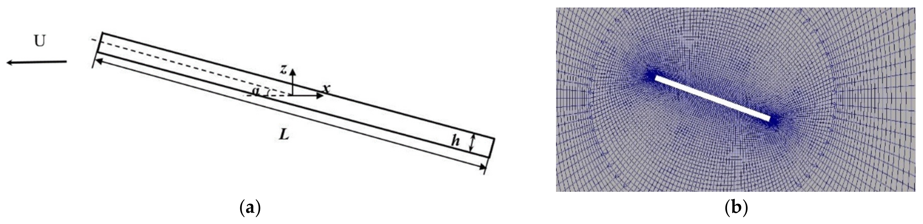
where, $U$ is the uniform free stream velocity at infinity, $n$ is external normal to the surface, $\mathsf{\Sigma }$, of the obstacle with length, $L$, and height, $h$.

The governing Equation (1) and the boundary conditions, Equation (2), are described by a set of length or time scales, $\left(\mathsf{\Lambda }, L, h\right)$, $\left(T_b, T_U^L=L/U\right)$, and parameters of the body motion or dissipative coefficients. The internal wave field and the flow fine structure are characterized, respectively, by large dynamic scales, such as internal wave length, $\lambda =U{T}_b$, and viscous wave scale, ${\mathsf{\Lambda }}_{\mathsf{\nu }}=\sqrt[3]{g\mathsf{\nu }}/N=\sqrt[3]{\mathsf{\Lambda }{\left({\mathsf{\delta }}_N^{\mathsf{\nu }}\right)}^2}$, and ligaments with transverse microscales, ${\mathsf{\delta }}_N^{\mathsf{\nu }}=\sqrt{\mathsf{\nu }/N}$, ${\mathsf{\delta }}_N^{{\mathsf{\kappa }}_S}=\sqrt{{\mathsf{\kappa }}_S/N}$, which are combinations of the dissipative coefficients and buoyancy frequency, similar to the Stokes scale on an oscillating surface, ${\mathsf{\delta }}_{\mathsf{\omega }}^{\mathsf{\nu }}=\sqrt{\mathsf{\nu }/\mathsf{\omega }}$ [35,36,37,38,39,40]. Another type of ligaments with Prandtl’s and Peclet’s scales are defined as relations of the dissipative coefficients and velocity of the body motion, ${\mathsf{\delta }}_U^{\mathsf{\nu }}=\mathsf{\nu }/U$ and ${\mathsf{\delta }}_U^{{\mathsf{\kappa }}_S}={\mathsf{\kappa }}_S/U$.

Relations of the basic length scales produce a set of typical dimensionless numbers and parameters, such as, Reynolds, $\mathrm{Re}=L/{\mathsf{\delta }}_u=UL/\mathsf{\nu }$, internal Froude, $\mathrm{Fr}=\lambda /2\mathsf{\pi }L=U/NL$, Péclet, $\mathrm{Pe}=L/{\mathsf{\delta }}_{\mathsf{\rho }}=UL/{\mathsf{\kappa }}_S$, sharpness factor, ${\mathsf{\xi }}_p=L/h$, and some other specific ones for a stratified medium, including length scales ratio, $C=\mathsf{\Lambda }/L$, as an analogue of the reverse Atwood number, ${\mathrm{At}}^{-1}=\left({\mathsf{\rho }}_1+{\mathsf{\rho }}_2\right)/\left({\mathsf{\rho }}_1-{\mathsf{\rho }}_2\right)$, for a continuously stratified fluid.

Such a variety and difference in values of the typical length scales of the problem under consideration indicate complexity of the flow structure around an obstacle for all the flow regimes, starting from the creeping and up to the unsteady vortex one. The large length scales prescribe necessary selection conditions for dimensions of the observation or computation domains, which should contain all the basic structural components, such as upstream perturbations, downstream wake, internal waves, and vortices. The microscales predefine spatial and temporal resolution for the numerical simulation and experimental facility. In the creeping flow regime, the Stokes scale is a critical one, while in the unsteady vortex regime, the Prandtl’s scale is dominant.

3. Numerical Simulation

Numerical simulation of stratified flows has manifold challenges related to application of the most appropriate numerical schemes, pressure-velocity coupling algorithms, adaptive mesh approaches, no-reflective boundary conditions at external boundaries, optimization of numerical procedures, high performance computing, etc. Since studies on stratified flows are of a great fundamental and practical interest, the most of these numerical problems have been successfully solved using computational packages or program codes of own development [42,43,44]. In the present study, numerical simulation for the formulated mathematical problem is constructed on the basis of the finite volume method using the computational utility OpenFOAM [45]. The open source of this computational package enabled us to create original program codes of our own development in the C++ environment for modifying and improving the existing approaches and standard solvers for numerical simulation of stratified flows in order to be able to perform direct numerical simulation in a wide range of Reynolds and Froude numbers. More detailed information on the modifications made to the standard OpenFOAM solvers one can find in other papers by the authors [35,36,37,38,41].

The general numerical approach used consists in discretization of the convective terms and time derivatives in the governing equations with second and higher-order numerical schemes. For numerical solving the resultant system of linear equations obtained due to the discretization of the governing differential Equation (1) with the boundary conditions [Equation (2)], conjugate or bi-conjugate gradient methods with preconditioning are used together with the modified iterative PIMPLE algorithm for pressure-velocity coupling [45]. The computation domain is discretized by a block structured mesh with a grading towards the surface of an obstacle, which is first constructed coarse and then locally refined based on the adaptive mesh techniques or sequential iterative procedures.

The additional mesh refinement is implemented in order to adequately take into account the viscous, diffusion and stratification effects, especially in the near-wall region, and to provide an adequate resolution of the finest flow elements in the most perturbed flow region around the body. The general draft of the problem under consideration and fragment of the computational mesh before additional refinement are shown in Figure 1. The calculations are performed with time step, $\mathsf{\Delta }t$, which is related to the minimal dimension of mesh cell, $\mathsf{\Delta }r$, with local flow velocity v by the Courant condition, $\mathrm{Co}=\left|v\right|\mathsf{\Delta }t/\mathsf{\Delta }r\le 1$.

External dimensions of the computational domain are evaluated on the basis of a series of numerical experiments as to meeting the criterion for the least disturbing effect of the uniform free stream conditions on the flow structure. In the present numerical simulation, optimal dimensions of the computational domain were predefined to be about 10 × 5 lengths of the plate. In order to satisfy all the mentioned conditions for the numerical simulation, the total number of computational cells must be about 2 × 10⁶ even for the 2D problems being solved in this study. Additional numerical control is provided by comparison of independent calculations for stratified fluids with different values of buoyancy frequency, including the degenerated case of actually homogeneous fluid.

The need for high spatial and temporal resolution of the finest flow components in the numerical simulation constructed for solving the problems under consideration forces us to search optimal ways to significantly shorten the computational time. So, the computations were performed in parallel regime using powerful multicore personal computers and computing resources of cluster systems, including the Federal collective usage center [Complex for Simulation and Data Processing for Mega-Science Facilities at the NRC “Kurchatov Institute”. Available online: http://ckp.nrcki.ru (accessed on 30 August 2021)].

4. Laboratory Modeling

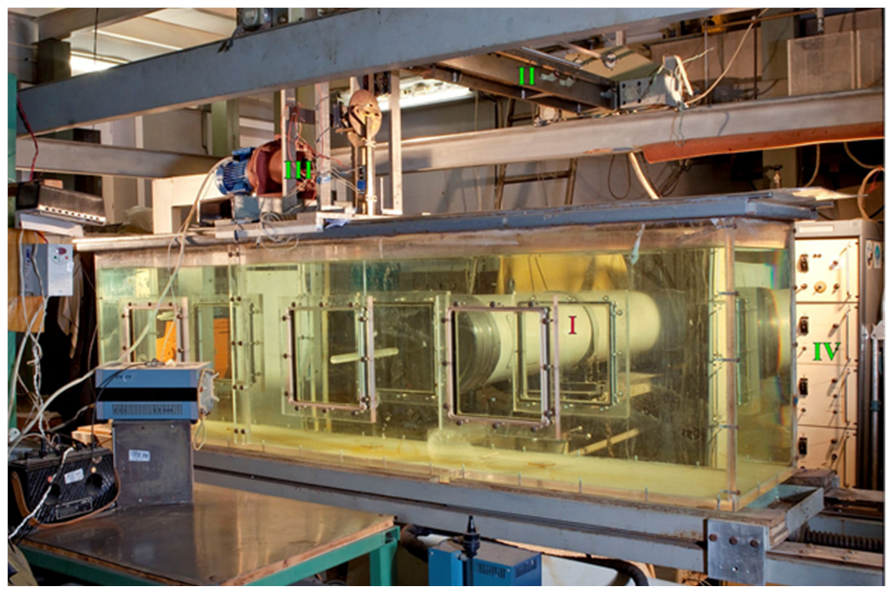
The laboratory experiments were conducted at the stand “Laboratory Mobile Tank (LMT)”, as a part of the Unique Science Facility “Hydrophysical Complex of the IPMech RAS” for modeling hydrodynamic processes in the environment and their impact on underwater technical objects, as well as distribution of impurities in the ocean and atmosphere (USF HPC IPMech) [46]. The laboratory setup includes a tank with dimensions of 220 × 40 × 60 cm³ and additional devices for filling with a stratified fluid, towing models, generating surface and internal waves, placing and moving sensors, sonar, flow visualization, experiment control and data processing. For the simultaneous use of several visualization methods (Schlieren interferometry, dyes, markers, etc.), the laboratory tank frame is made of plexiglass, and three pairs of optical windows are inserted along the long side of the tank. In order to reduce the influence of background perturbations, the tank is installed on vibration dampers and vibration damping inserts. A photo of the stand is shown in Figure 2.

The model towing system uses DC motor as a drive, which is connected to a drum pulling the drive cable through an electrofusion coupling and a two-way gearbox. The cable is attached to the carriage, which can be moved along the guides installed above the tank.

A plate is attached to the carriage using flat knives made of transparent plastic at an angle of attack, α, which can be continuously changed in the range $0÷90°$. The pulling system allows model towing with a speed of 0.01 ÷ 6.0 cm/s, which can be varied by smooth changing the engine speed and switching the gearbox. Speed control is carried out according to the time of passage of the control base, uniformity of the movement being controlled optically. Relative unevenness of the movement did not exceed 3%.

Working environment is tap water and stratified aqueous solution of common salt. The tank filling system, which includes two reservoirs, two pumps, and piping system with valves, enables creating two-layer, multi-layer or continuous stratification with a controlled density distribution. In these experiments, the laboratory tank was filled with a continuously stratified fluid using the technique of sequential displacement of the water layer from the bottom from two additional tanks. The laboratory experiments were conducted for the following values of buoyancy period of the stratified fluid, $T_b=2\mathsf{\pi }/N=7.5; 12.5; 17.4 \mathrm{s},$ which correspond to the buoyancy frequencies, $N=\sqrt{g/\mathsf{\Lambda }}=0.84; 0.50; 0.35 {\mathrm{s}}^{-1}$, and density gradients, $\mathrm{d}\mathsf{\rho }/\mathrm{dz}=72, 25.5, 12.5 \mathrm{kg}/{\mathrm{m}}^4$.

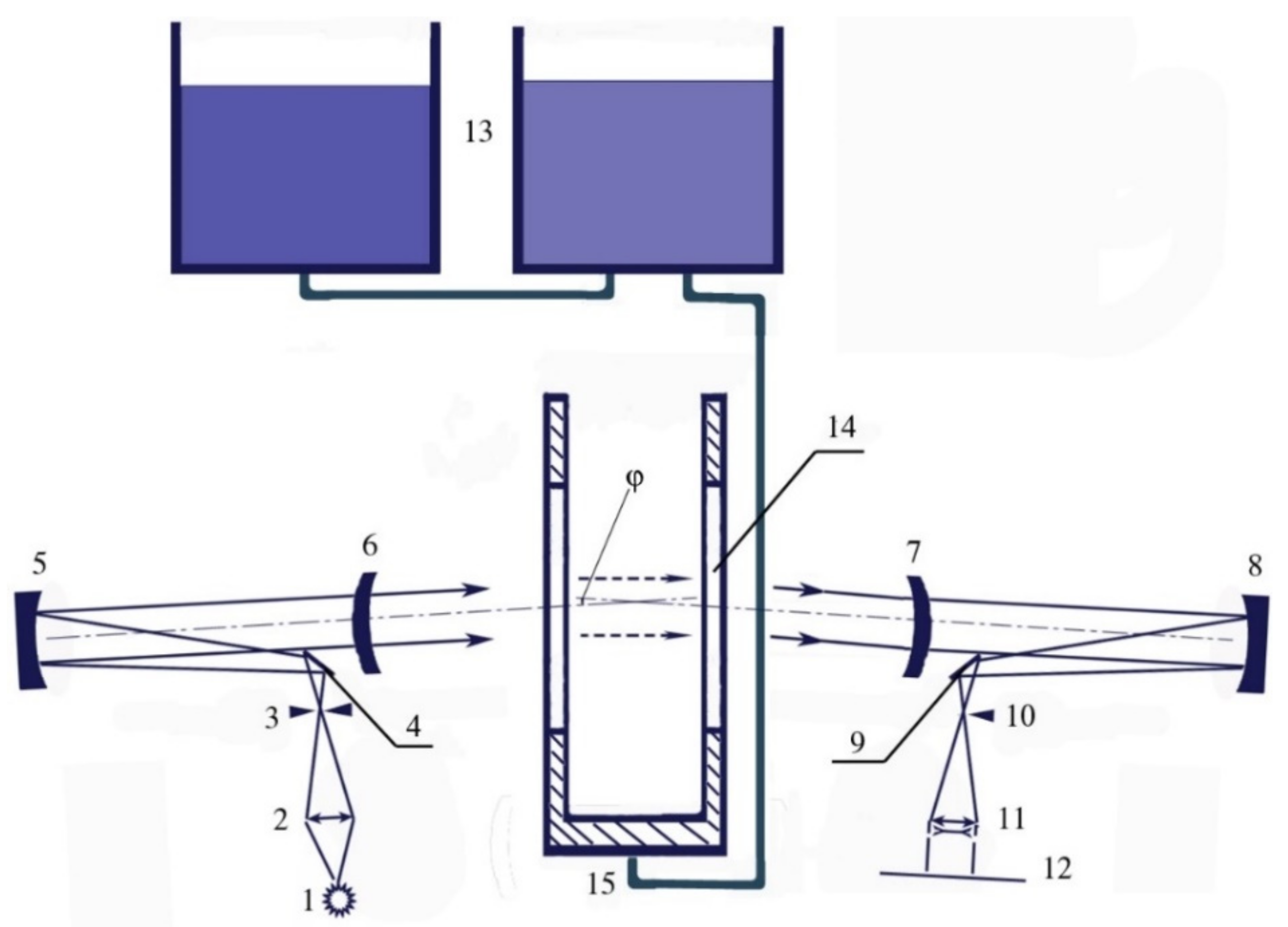
For flow pattern observation, the IAB-458 mirror Schlieren instrument was used with 23-cm-diameter view field and spatial resolution less than 0.05 mm [32]. A vertical slit was used as a lighting aperture with dimensions 10 × 0.2 mm². As a visualizing diaphragm, a flat vertical Foucault knife, Maksutov’s thread or regular grating to produce natural rainbow colour image of the flow were used [32,33]. A sketch of the facility is shown in Figure 3.

The optical system includes light source 1 (incandescent lamp); condenser 2 forming an image of the light source in the control diaphragm plane; lighting slit 3; flat rotatable mirrors 4, 9 directing light beams to the main spherical mirrors 5, 8; correcting menisci 6, 7; visualizing diaphragm 10 (thread, knife, grating); optical image conversion system 11, which builds an image of the studied flow pattern in the observation plane 12. Working solutions from reservoirs 13 enter the tank through holes at the bottom 15, covered with disks which turn the flow. Observations are carried out through windows 14.

Since the refraction index depends on the medium density, a tank with flat walls filled with a linearly stratified fluid is equivalent to an optical prism which turns the light rays by an angle $\mathsf{\phi }$. To compensate for the deflection of the rays, independent lighting and receiving parts of the Schlieren instrument are installed in the same vertical plane on supports which allow the height and angular position adjustment. The platform design gives room to implement the standard procedure for adjusting the Schlieren instrument when changing the stratification without resorting to additional optical devices, i.e., it can be selected the inclination angle of the instrument elements, their height, the mutual spatial and angular positions of the optical axes at the points of the beam outlet from the lighting part and its inlet into the receiving part.

The high sensitivity of the Schlieren instrument enables measuring the buoyancy period and the vertical profiles of the flow velocity using density markers. In the experiments, the markers are created by freely floating gas bubbles, submerged crystals of sugar or table salt. If the Reynolds number, ${\mathrm{Re}}_b$, defined by diameter, $d_b$, speed of movement of a bubble or a crystal, $U_b$, and kinematic viscosity of water, satisfies the condition, ${\mathrm{Re}}_b=\frac{U_b{d}_b}{\mathsf{\nu }}<200$, it moves uniformly, rectilinearly and leaves behind a vertical wake with a thickness of $\mathsf{\delta }~0.25 \mathrm{mm}$, forming a marker line which can be observed using the Schlieren instrument up to 90 s.

The sinking vertical wake excites natural medium oscillations with a typical buoyancy period, $T_b$ [47]. Variations in the medium density near the marker were registered by the Schlieren instrument or a high-resolution conductivity sensor. The marker displacements for a certain time interval, $\mathsf{\Delta }t$, were used to reconstruct the horizontal velocity component profile in a flow section under study. Some examples of the comparison of the calculated and observed marker displacements in the attached internal wave field past a plate are given in [12].

In the present experiments, a vertical slit illumination diaphragm and a flat vertical Foucault knife were used as a basic visualization facility. Illumination variations are proportional to changes in the horizontal component of refraction index gradient which, in turn, is in a linear relation to the fluid salinity and density for the case of aqueous sodium chloride solution used in the experiments to produce the stratification. The Schlieren image coloring is due to the light dispersion effects in a stratified medium [33].

5. Results and Discussion

In this section, instantaneous flow patterns around a horizontal and a tilted plate are studied numerically and experimentally for the cases of stratified and homogeneous media. Different flow regimes are considered, such as creeping, wave and unsteady vortex ones, which are characterized by their individual sets of dominating structural flow components, including up-stream perturbations, internal waves, vortices, and ligaments. The numerically calculated and experimentally visualized flow patterns around a plate are compared with each other for different flow conditions, fluid properties and plate parameters.

5.1. Creeping Flow Regime

Under the action of combined effects of a medium non-homogeneity and the Earth’s gravitation or rotation, a stable stratification is formed, which is characterized by natural molecular flux of a stratifying agent acting in the opposite direction to gravity. Being interrupted on the impermeable surface of a motionless obstacle, the diffusion flux gives rise to formation of fine structural diffusion-induced flows in an initially quiescent medium without any external mechanical reasons [41]. The stationary solutions for the problem on diffusion-induced flow on an infinite inclined plane, obtained by Prandtl [8], lose regularity at the horizontal position of the plane, but the complete numerical solution of the Equation (1) for unsteady flow remains finite for any tilt angle of an obstacle and gives room to obtain solutions for arbitrary geometry of the body [36,37,41].

The diffusion-induced flow around a horizontal plate consists of multilevel convective circulation cells with a symmetric structure relative to the central vertical plane, which is kept similar for all the physical variables, but thickness of separating interfaces is individual for each variable. 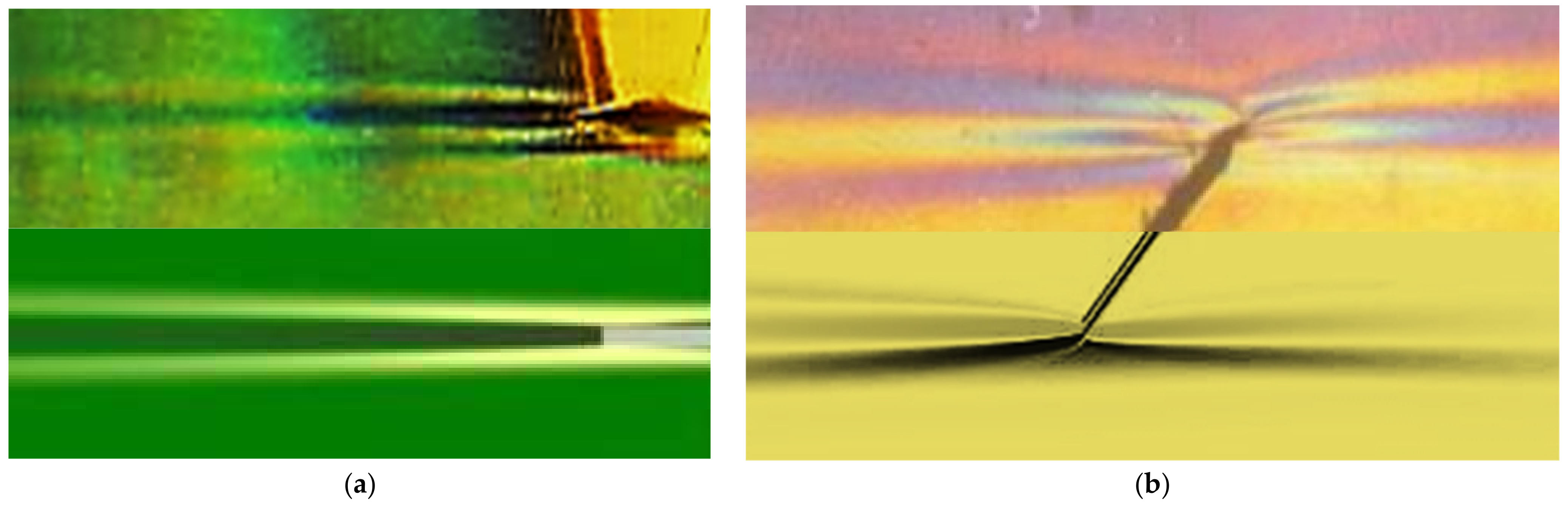Even a small deviation from the horizontal position of the motionless plate breaks the flow symmetry with formation of both ascending and descending flows along the upper and lower surfaces of the plate [36,37,41]. Around the plate edges at an arbitrary tilt angle, the diffusion-induced flow is mainly manifested in the form of horizontal streaky structures capable of extending over great distances from the obstacle, which are clearly visualized in the laboratory experiments by Schlieren instruments [33,34]. (Figure 4). The numerical and experimental results on the diffusion-induced flows around a horizontal plate and a tilted one are in a good agreement between each other, as can be seen from the comparisons in Figure 4a,b.

Slight differences in the flow fine structure patterns around the plate edges are caused by differences in the problem statement in theory and experiments. In the numerical simulation, the fluid is assumed to be at rest, but in practice, some random disturbances, caused by movement of nearby heavy traffic, subway trains and other external factors, lead to vibrations of the tank and create slow flow unsteadiness, despite all efforts to stabilize the tank position. The flows, which were not registered in these experiments, are manifested in some variability of the flow fine structure in the chlieren images near the plate edges.

5.2. Wave Flow Regime

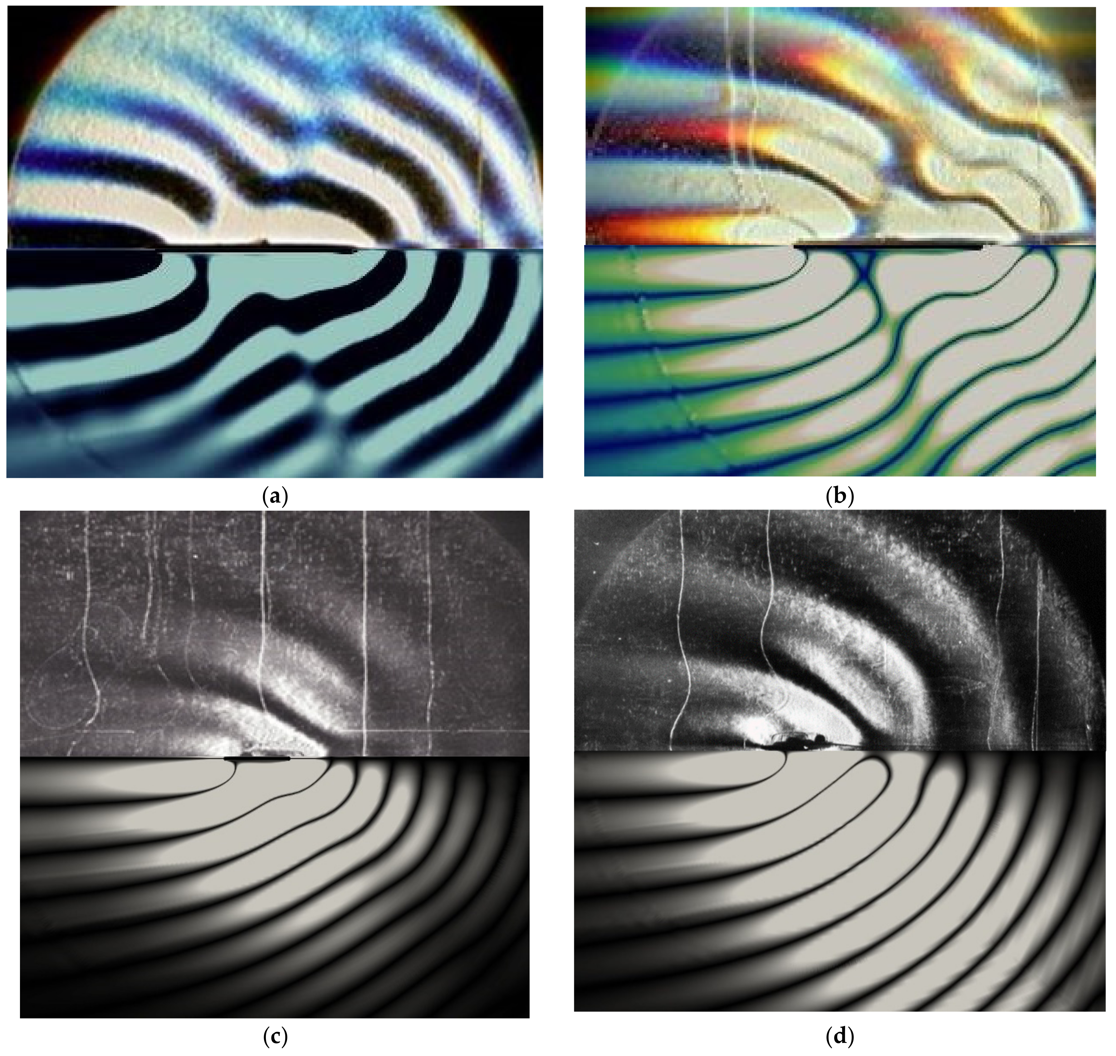
With instantaneous start of uniform movement of a body in initially quiescent stratified fluid, vertical displacement and entrainment of the surrounding fluid by the moving body cause fluid oscillations around initial neutral buoyancy horizons with characteristic buoyancy frequency, which, in turn, trigger the mechanisms for formation of internal wave fields, such a wide-spread phenomenon in the Earth’s atmosphere and hydrosphere.

At relatively low Reynolds numbers, a typical stratified flow pattern around a moving body consists of specifically arranged groups of upstream perturbations and attached internal waves. Phase surfaces of the internal waves separate half-waves of crests and troughs which bind towards horizons in front of the body and close up behind the body. The calculated and visualized internal wave patterns around a horizontal plate with lengths, $L=2.5 \mathrm{cm}$ and $L=7.5 \mathrm{cm}$, moving with different velocities in a stratified fluid are presented Figure 5.

For all the cases considered, perturbation sources at the edges of a uniformly moving plate generate regular and smooth wave fields with their intensity decreasing with growing distance from the moving body. However, in the case of the longer plate, the phase surfaces of the internal waves are broken above and beneath the plate, since, for this case, the internal wavelength, $\lambda =U{T}_b$, turns to be smaller than the plate length ($\lambda <L$). The comparisons in Figure 5 show the numerical and experimental data are in a good qualitative agreement of the calculated and visualized internal wave fields.

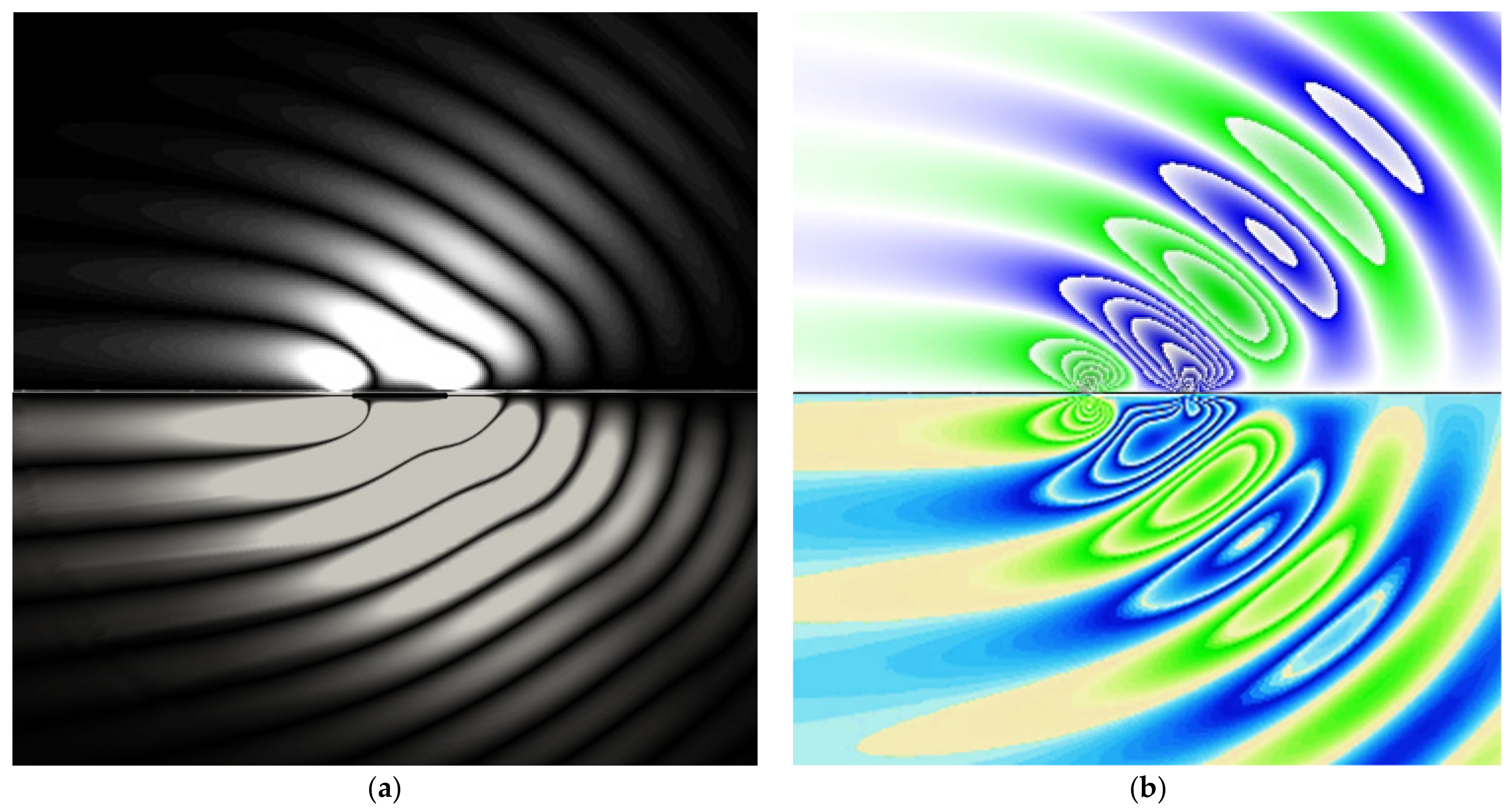
The problem on uniform movement of an obstacle in a stratified medium allows obtaining exact solutions with certain strict limitations, which include linearization of the governing equations, applying no-slip boundary conditions along the whole trajectory of plate movement (the underlying plane approximation), and numerical visualization of the final analytical expressions [34]. In Figure 6, the results of direct numerical simulation and analytical solution for the problem on internal wave field generation by a horizontally moving plate are presented in the synchronized image with the upper and lower halves corresponding to the numerical and analytical results, respectively.

Although there is a good agreement of the far flow field structures away from the plate, one can see noticeable differences around the movement trajectory past the plate and in the upstream perturbation, which are caused by the no-slip boundary conditions imposed on the movement trajectory in the analytical solution. There are also some differences in the structure of regional singularities, especially near the trailing edge of the plate, where a moving obstacle in the free space produces less intensive perturbations. In general, the numerical and analytical results are in a good agreement and reflect all the basic flow components which are observed in the laboratory experiments.

Instantaneous patterns of the stratified flow structure around a horizontal plate and a tilted one in the wave regime is presented in Figure 7, which demonstrate the flow structure evolution in time. The process of formation and evolution of the internal wave structure around a tilted plate goes through a number of specific unsteady stages. Initially, four groups of internal waves emerge at the sharp edges of the plate, where the most intense shifts of fluid particles from the neutral buoyancy horizons occur. Then, the internal waves propagate from the perturbation sources that is accompanied by the interaction of individual wave fields with each other and with the surface of the plate. Under the action of the free stream, the wave perturbations on the windward side of the plate are suppressed, and two groups of internal waves generated by the sharp edges of the trailing edge of the plate are merged into a single one.

At the same time, the vortex wake appears on the leeward side of the plate and starts interacting with the generated internal wave fields. And, finally, goes a stabilization process of the upstream perturbation structure in front of the plate and the attached internal wave fields behind the obstacle against the background of the unsteady vortex wake. In the particular case of the horizontal plate, the flow structure evolution takes the simplest form, which is symmetric relative to the plane of the plate movement. So, fluid flows around obstacles can be treated as evolving sets of multiscale flow components, such as waves, vortices, and ligaments, being in a continuous spatial-temporal interaction with each other, rigid boundaries, and free stream.

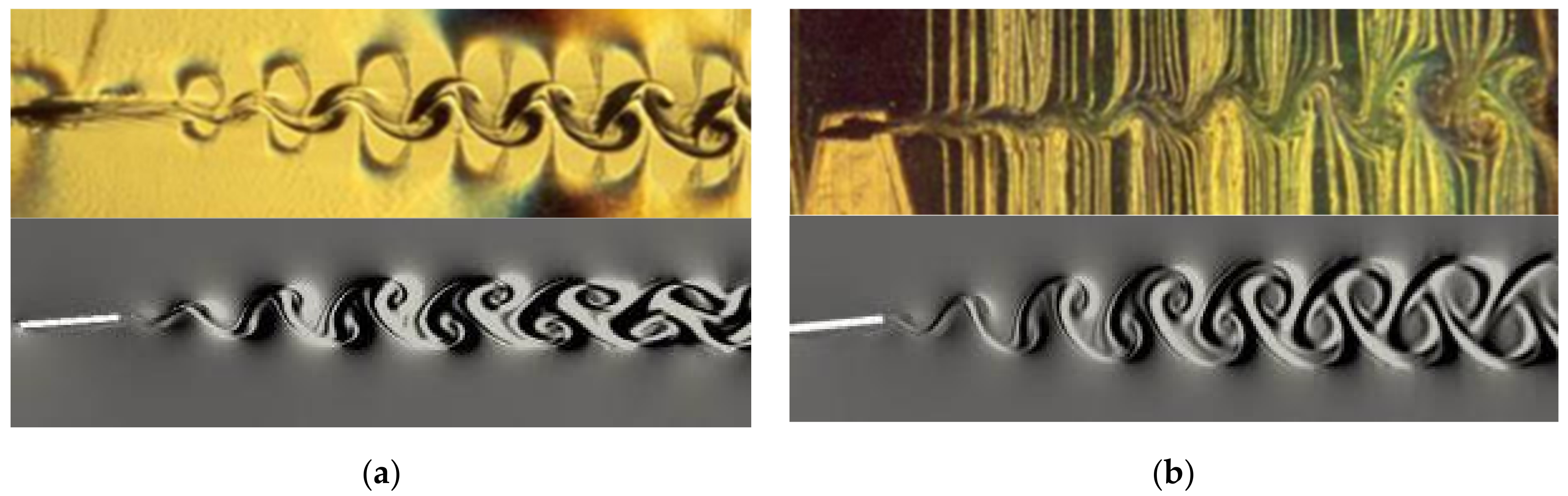
In the calculated and schlieren visualized patterns of stratified flows around a vertical plate, all the structural elements of the stratified flow are well manifested, including slowly evolving ones, such as fields of attached waves, upstream perturbations, and vortex wake past the obstacle, and rapidly changing ones, such as fine structural interfaces (ligaments), and their sets: Vortices (Figure 8). In an unsteady flow, all the flow components are represented simultaneously and manifested to various degrees, actively interacting with each other and with the free stream [38].

The slow body motion regime is characterized by coexistence of different flow structural components, such as rays of upstream oblique internal wave, attached internal waves past the body, and ligaments, which are formed at a distance from the plate edges and bound the density wake (Figure 8a). In the intense wave regime, there are both waves and an extensive family of ligaments which form a thin-layered wake (Figure 8b,c). Both the calculations and experiments register fine structural elements in the upstream perturbation, which indicates existence of ligaments both past and in front of the body. As one can see from the comparisons of the visualized and calculated flow patterns, the attached internal wave phase surfaces are deformed by the wake flow a bit stronger in the experiments as compared to the computations, and the splitting process of thin-layered flow elements is more pronounced.

Further increase in the velocity of the vertical plate movement leads to a certain restructuring of the general flow structure, including leaning of the internal wave phase surfaces towards the direction of the body motion, significant change in form and scales of the fine-structural flow elements, and manifestation degree of individual flow components (Figure 8d). There are essential structural changes observed in the wake past the plate with formation of typical vortex elements, including vortex dipoles past the body or “vortex bubbles”, especially in the flow regions where the internal wave phase surfaces diverge. The calculations and observations of the flow patterns are in a good qualitative agreement with each other in all the flow regions, including the upstream perturbations, a system of internal waves, the downstream wake with fine structures and vortices.

5.3. Votrex Flow Regime

In an unsteady flow, all the flow components, including slowly evolving upstream and attached wave fields, and rapidly changing fine-structured layers or ligaments, are in a continuous active mutual interaction, affeced by bounding surfaces and free stream. Figure 7b and Figure 8d demonstrate the situation when internal waves, ligaments and vortices coexist simultaneously in the same flow and actively interact with each other. In the pure vortex flow regime, when the vortex elements become a dominant flow component with the internal wavelength comparable to the observation area size, the most contrast structural changes are manifested in the wake flow past the plate (Figure 9).

Both laboratory and numerical simulations show that the wake flow structure past the tilted plate consists of a typical vortex street in the form of a sequence of mushroom-like elements. In the strongly stratified medium (Figure 9a), the wake vortices gradually collapse downstream, being broken up into a set of fine-structural elements, while in the homogeneous fluid (Figure 9b), the vortex street expands, while evolving downstream, in the vertical direction within the observation area. A variety of multilayer fine-structural flow elements is formed on the vortex shells and in the regions of interaction of the vortex flow multiscale components between themselves and with the plate surface.

5.4. Unsteady Votrex Flow Regime

The greatest scientific and practical interest is in studying the unsteady vortex regime of stratified flows when internal waves, vortices and fine structural ligaments, are in an intensive unsteady mutual interaction. At certain combinations of values of the problem parameters, some of the flow components can be substantially prevailing over other ones, and the general flow structure seems to be stable or even (quasi-)stationary. However, at other values of the problem parameters, multiple mutual interactions of different-scale vortex elements and ligaments may produce an essential flow unsteadiness [35,36,37]. In the unsteady vortex regime, upstream and attached internal waves are far from a dominant flow component with internal wavelength much larger than the visualization area size, but their interactions with vortex elements can affect the flow fine structure.

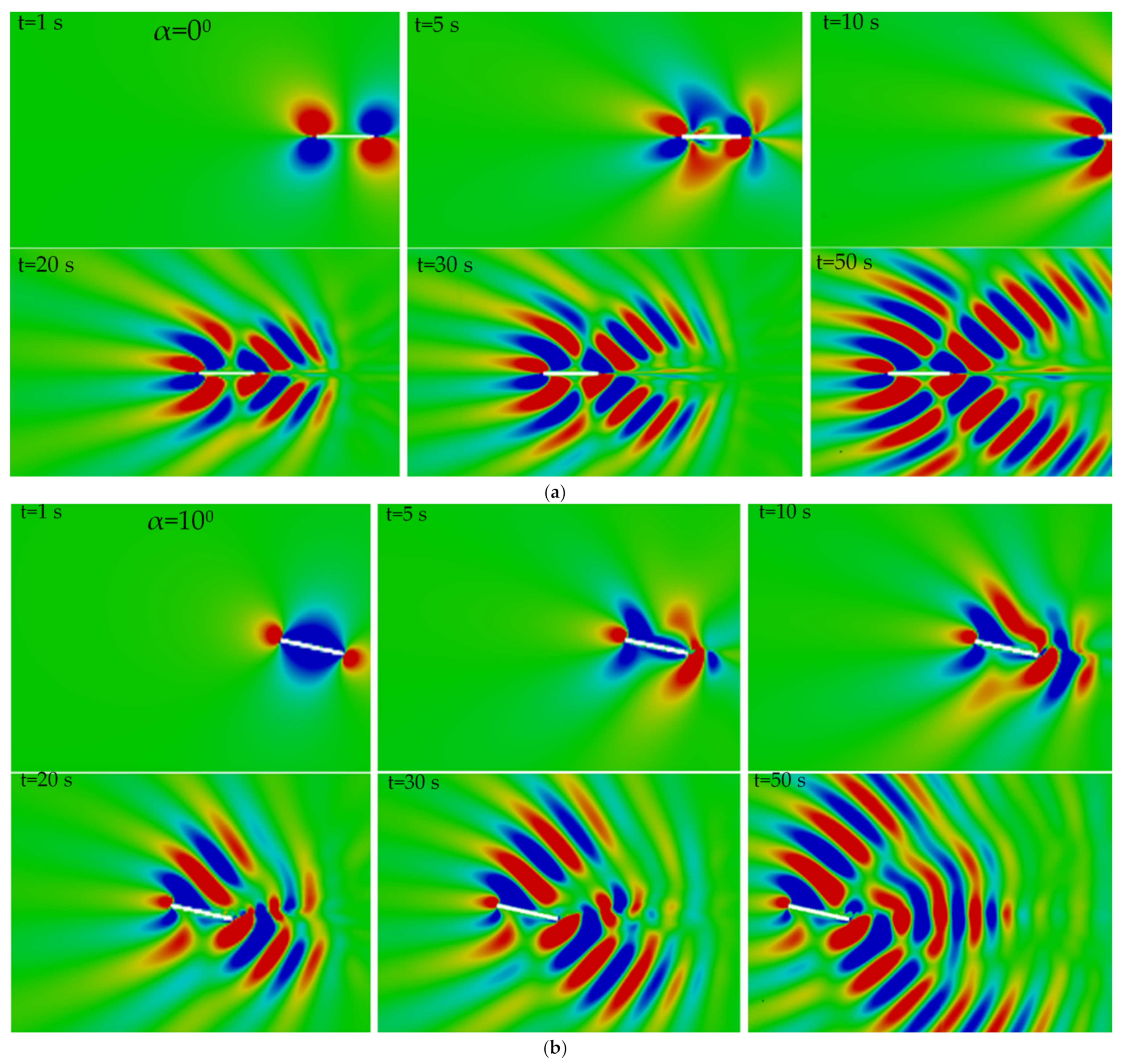
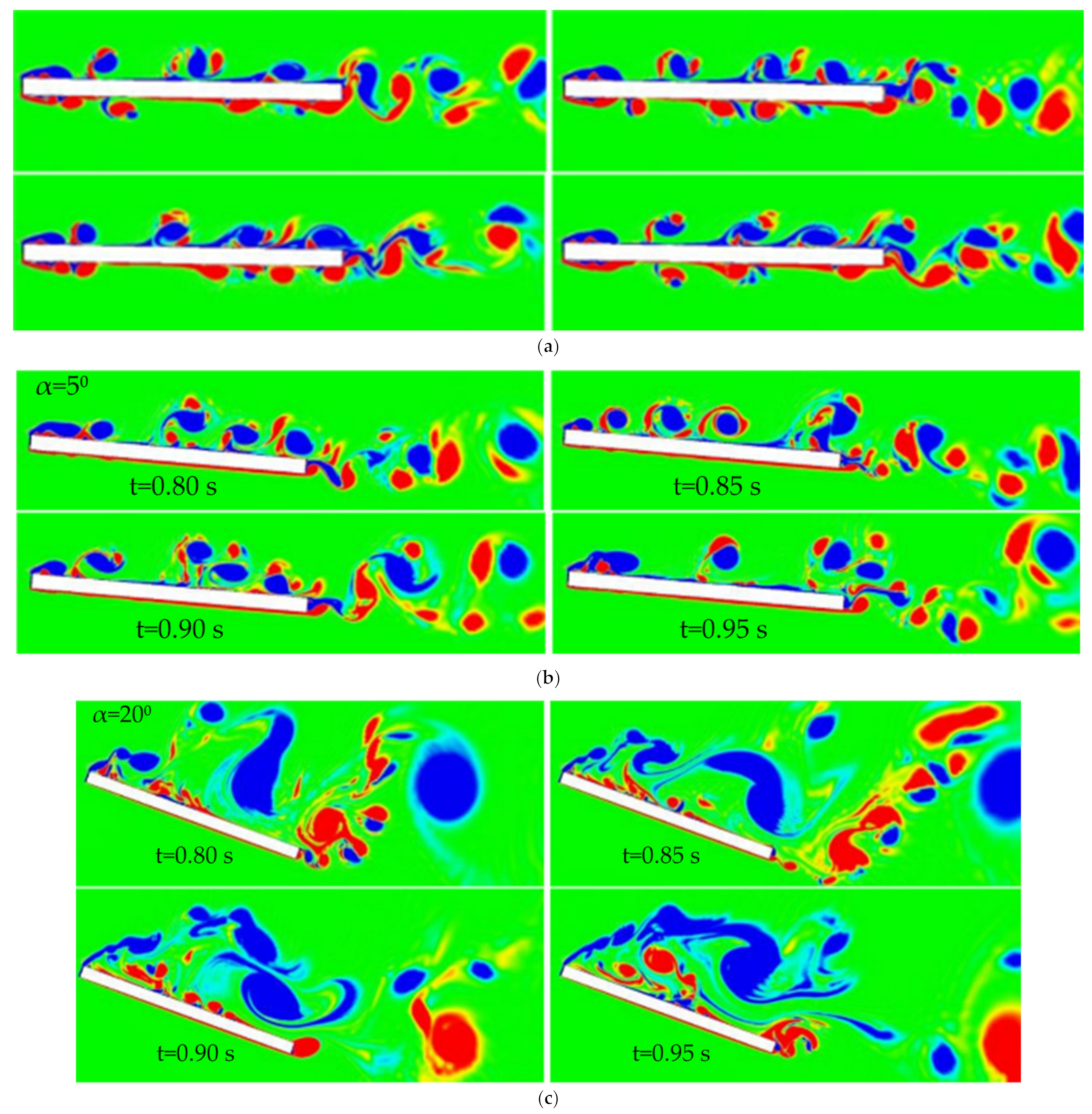
Iinstantaneous vorticity field patterns for different tilt angles of a horizontally moving plate, which demonstrate complex mutual interactions of multi-scale flow components, is shown in Figure 10. Here, the unsteady flow evolution is presented by four instantaneous vortex flow patterns for each considered value of tilt angle at sequential time instances with interval of 0.05 s. Red and blue colors in the color spectrum correspond to positive and negative values of the vorticity field within the range, $-100<\mathsf{\omega }<100 {\mathrm{s}}^{-1}$, and green color corresponds to zero value of vorticity.

The vortex flow structure at small values of tilt angle of the plate movement consists of two quasi-steady chains of leading-edge vortices, which drift along the upper and lower sides of the plate, gradually dissipating as moving downstream (Figure 10a). In the wake flow past the plate, there are intensive interactions of the drifting leading-edge vortices and the primary vortex street with typical scales comparable to the plate’s thickness. This results in a loss of the initial quasi-steady vortex shedding structure and formation of a new less regular one with a frequency of about two times lower than the primary value.

At larger tilt angles of the moving plate, the flow pattern loses the primary symmetry relative to the free stream direction, and the flow vortex structure, scales and intensity on the windward and leeward sides of the plate become essentially different (Figure 10b). The chain of leading-edge vortices, which have more pronounce forms and larger scales as compared to the case of small tilt angles, drifts downstream at a somewhat greater distance from the leeward side of the plate. The vortex dynamics on the windward side is significantly suppressed by the encountered fluid, so that only weak flow perturbations are observed in the shear layer. Like in the previous case, the quasi-steady vortex shedding past the plate at large time instants are formed by interaction processes of the leading-edge vortices with the primary regular vortex shedding past the plate.

With further increase in tilt angle of the plate, the vortex flow dynamics on its leeward side is essentially intensified with loss of the regularity of leading-edge vortex formation and evolution downstream, as compared to the cases of smaller tilt angles (Figure 10c). While the flow region on the windward side is completely unperturbed due to the suppressing effect of the oncoming free stream, on the opposite side a sequence of more complicated and intensive clockwise rotating vortex elements are formed by involving in a large-scale rotating motion chains of two or more leading-edge vortices. As this compound vortex moves further downstream towards the trailing edge of the plate, a new counter-clockwise rotating large-scale vortex structure is formed around the trailing edge with its shell comprised of chains of the vortex shedding elements. So, with increase in tilt angle of the plate, the vortex flow structure tends to formation of two interacting counter rotating large-scale vortices comprised of leading-edge vortex chains and wake vortex street respectively.

The fields of different physical variables included into the governing system of Equation (1) together with their combinations and gradients allow versatile studying the physical processes under consideration. In its turn, this enables collecting the most comprehensive information on the physical mechanisms involved in the processes under study.

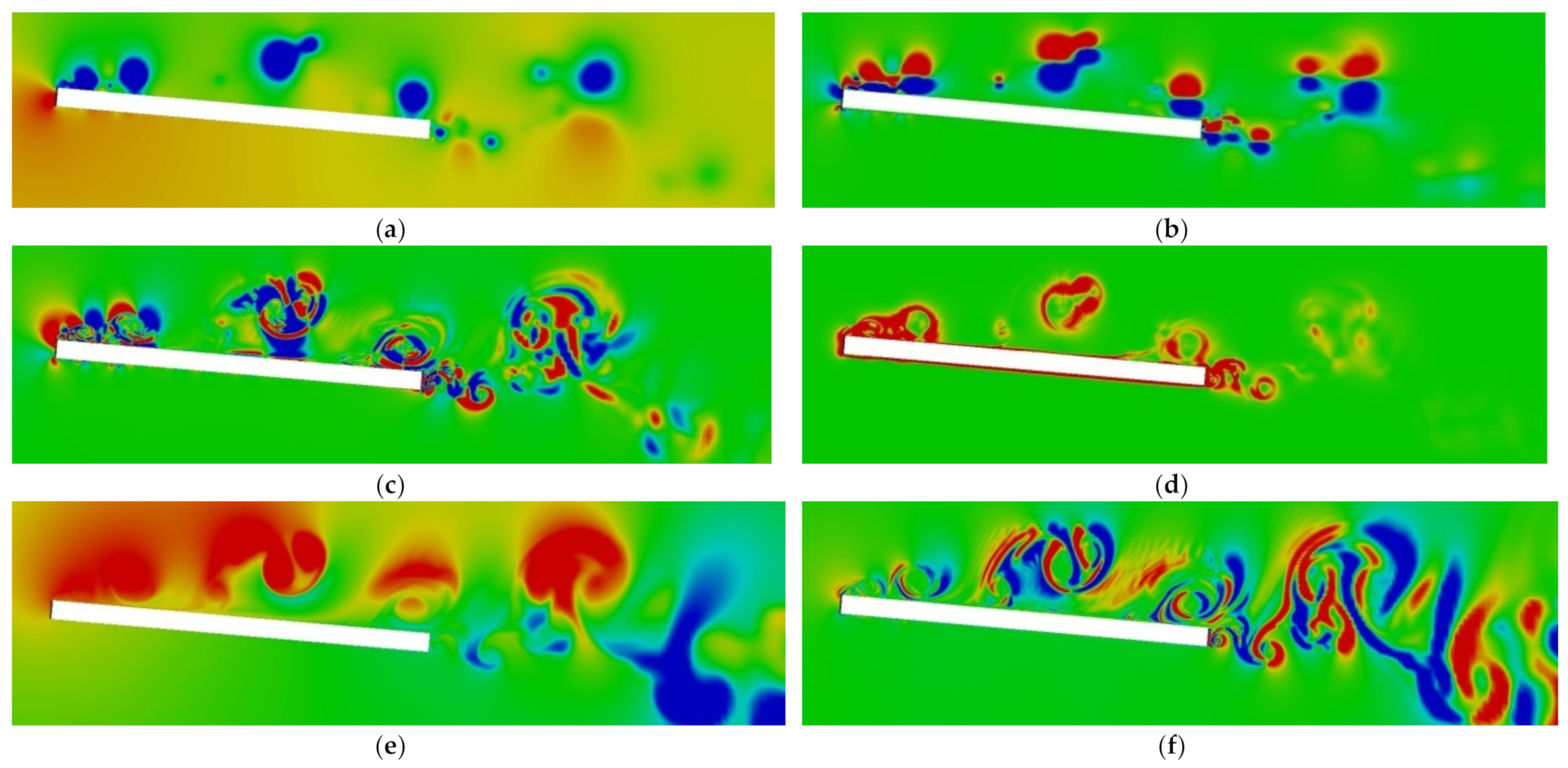
Calculation of the pressure field is of a particular research and practical interest, since in the traditional description noticeable restrictions are imposed on this variable [9,10,35]. It may be qualitatively noted that the stratification affects this flow field only slightly, while the transverse dimension of the obstacle produces a strong impact observed in the experiments [35]. In the patterns of pressure field shown in Figure 11a, there is a pressure increase in the upstream perturbation in front of the plate, strong rarefaction spots in the divergent flow near the leading edge, and a pressure deficiency in the regions of localization of vortex elements. At the other parameters fixed, the vortex size depends on the plate thickness: for a thin plate, they take the form of vortex filaments, and for a thick one, they look like crosswise bands, as those observed in the experiments [32,34].

In the pattern of vertical velocity component, the upstream perturbation is expressed in the form of two spots with different signs at the sharp corners of the leading edge of the plate as a result of intensive fluid displacement in this zone (Figure 11b). Every vortex element in the leading-edge vortex chain and wake vortex street is presented by a pair of spots with opposite flow direction. There is a noticeable asymmetry of the spots in localizations of the vortex structures, which can be explained by the essential flow unsteadiness.

Calculation of the baroclinic vorticity generation rate field is of a particular interest, which has the most complex geometry in inhomogeneous fluid flows and is defined by the pressure and density gradients, $\dot{\Omega }=\nabla P\times \nabla \left(1/\mathsf{\rho }\right)$ (Figure 11c). The vorticity generation regions are pronounced near the leading edge, namely, at the upper edge with a scale of the order of the plate thickness and at the lower one with a much smaller size. Further downstream, the structures become thinner and elongated, mainly localizing on the shells of vortex elements in the form of multiple thin zones of vorticity amplification and decay. In the wake region past the plate, small-scale inhomogeneities of the field are manifested in the elements of the vortex street near the trailing edge, and in the far wake flow, relatively large inhomogeneities of both vorticity generation and dissipation are expressed as a result of the interaction of the leading-edge vortices with the external free stream. The geometry of this parameter can explain the dynamics of the vortex flow fine structure formation and the mechanism on the flow splitting into multilayered elements observed in the schlieren images of flows past a strip.

The mechanical energy dissipation rate is different from zero in a relatively narrow area in front of the plate, where the horizontal flow around the body is split, as well as in the shear layers on the windward and leeward sides of the plate (Figure 11d). The energy dissipation rate also reaches significant values on the vortex element shells, but these values tend to decrease as the vortices move downstream.

In the density perturbation field, the flow region expanding with distance from the leading edge is most clearly expressed, outlined by the lower edges of the spots of partially mixed fluid in vortices (Figure 11e). Above the plate, there is a layer with positive values of density perturbation, and below the obstacle, there is a layer with negative ones, due to the fluid transfer from equilibrium horizons by the drifting vortices. Regions with a weakly perturbed density distribution are adjacent to the trailing edge of the plate.

In addition to the density perturbation field pattern, analysis of the density gradient fields would be very useful, as well, since they can provide us with additional information on the flow fine structure not visible in the fields of other physical variables. The horizontal component of the density gradient is in a linear proportion to the light refraction ratio, which is visualized in laboratory experiments using Schlieren instruments and give a chance to clearly observe a wide variety of flow components, such as upstream perturbations, wake flows, vortices, internal waves, and ligaments [30,31,32,33,34].

The Schlieren images of light refraction ratio and calculated patterns of horizontal component of density gradient field presented in Figure 4, Figure 5, Figure 8 and Figure 9 demonstrate that the stratified flow fine structure comprises multifold of thin multi-layered structural elements with alternating signs, which outline vortex shells, demarcate flow regions with strong non-linear interactions, separate different multi-scale flow elements, etc. The fineness of the flow structural elements in the horizontal component of density gradient field patterns can be explained by large values of the ratio between the viscosity and diffusion coefficients, that is the Schmidt number, for the stratified fluid types considered in this study.

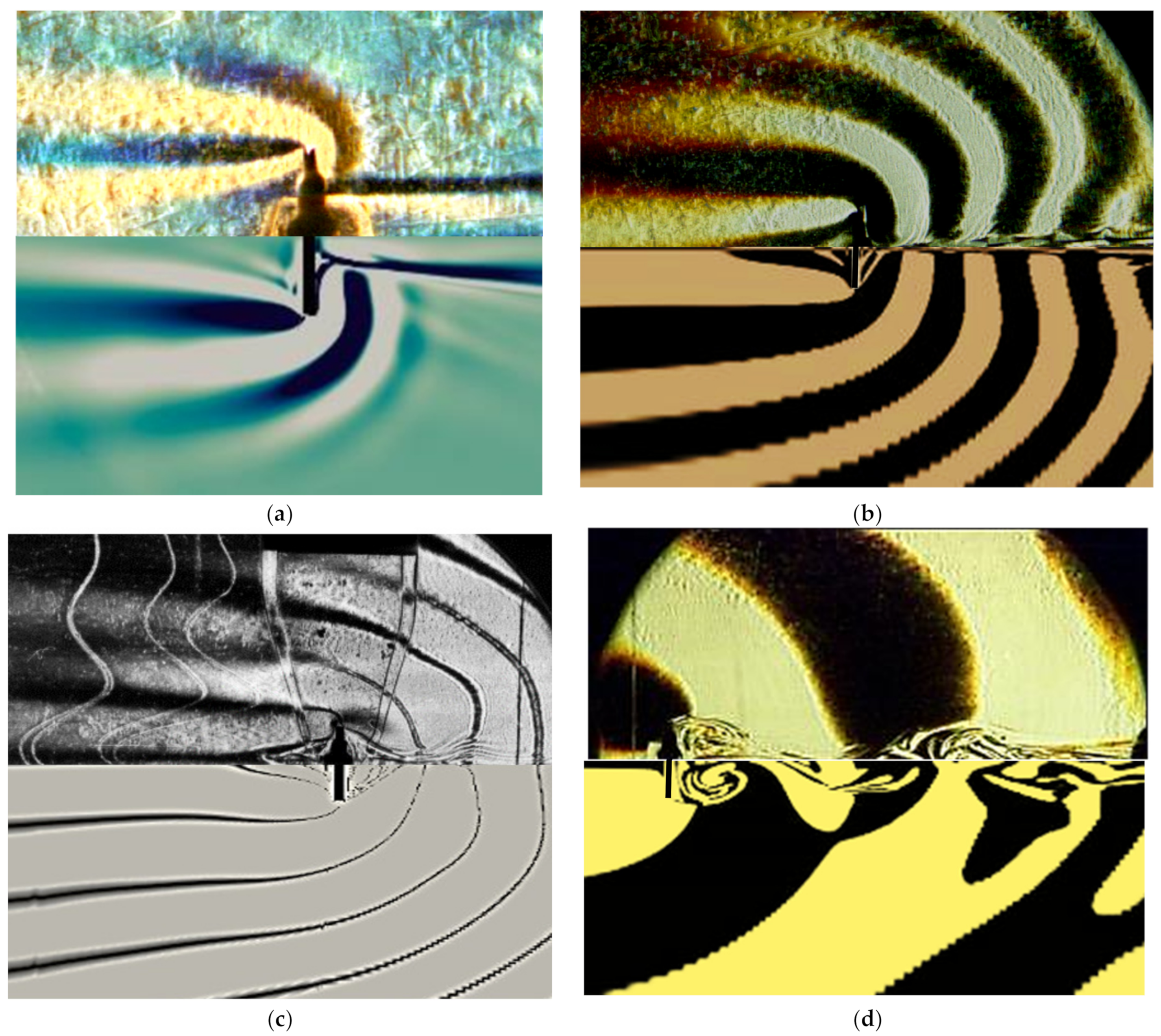
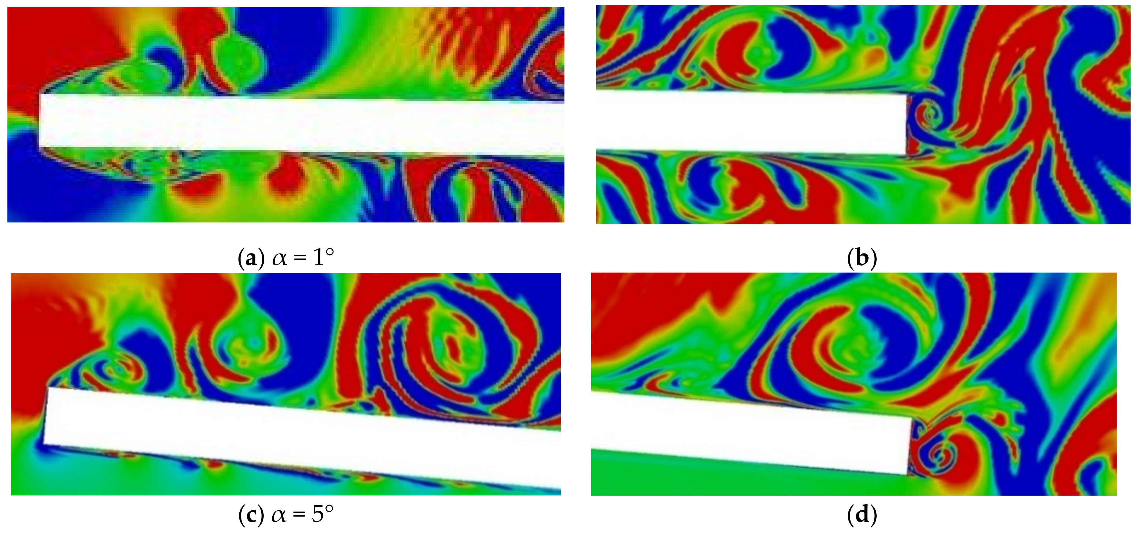
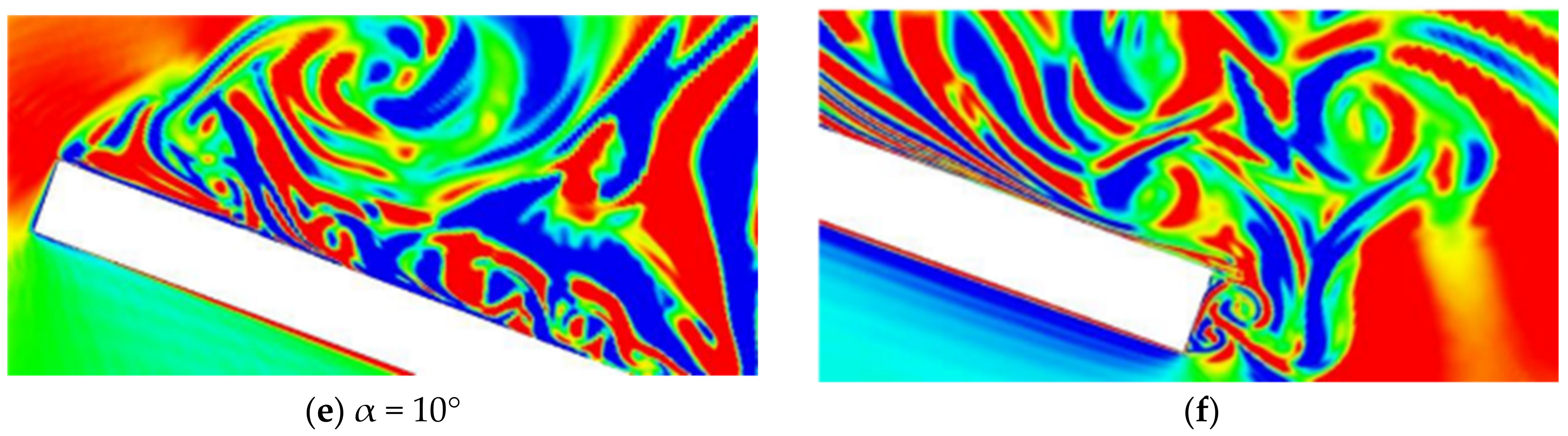
The finest structural elements are localized mostly around the plate edges, where the most intensive processes of generation and mutual interactions of multiscale flow elements occur. Instantaneous patterns of the horizontal component of the density gradient field around the leading and trailing edges of the tilted plate are presented in Figure 12 for three tilt angles to horizon. General structure of this field consists of thin layers of both signs, which are localized mostly on the vortex shells and gather into compact spots in the wake flow past the body.

At small tilt angles of the plate, systems of spiral curls and fine layered structures are formed on the cores of the leading-edge vortices around the sharp corners of the leading edge of the plate. As the leading-edge vortices move downstream, these fine structural elements get longer and thicker taking more complicated and distorted shapes, especially in the flow region past the trailing edge of the plate where an active mutual interaction of the leading-edge vortices with the vortex street occur (Figure 12a).

Further increase in tilt angle of the plate leads to a certain complication of the field structure with the typical layered elements being shortened, thinned and increased in number due to intensification of mutual interactions of the leading-edge vortices and their evolvement into complex larger-scale vortex structures (Figure 12b). At large tilt angles, the horizontal component of the density gradient field pattern contains sets of multilayered fine-scale elements located in the direct vicinity of the front side of the plate due to intensive interactions of the leading-edge vortices and large-scale vortex elements with the plate surface (Figure 12c). Both the numerically calculated and experimentally visualized flow patterns show that ligaments, together with waves and vortices, are an important fine-scale and high-gradient structural element of stratified flows, which exist in flow regions with intense non-linear mutual interactions of the flow components.

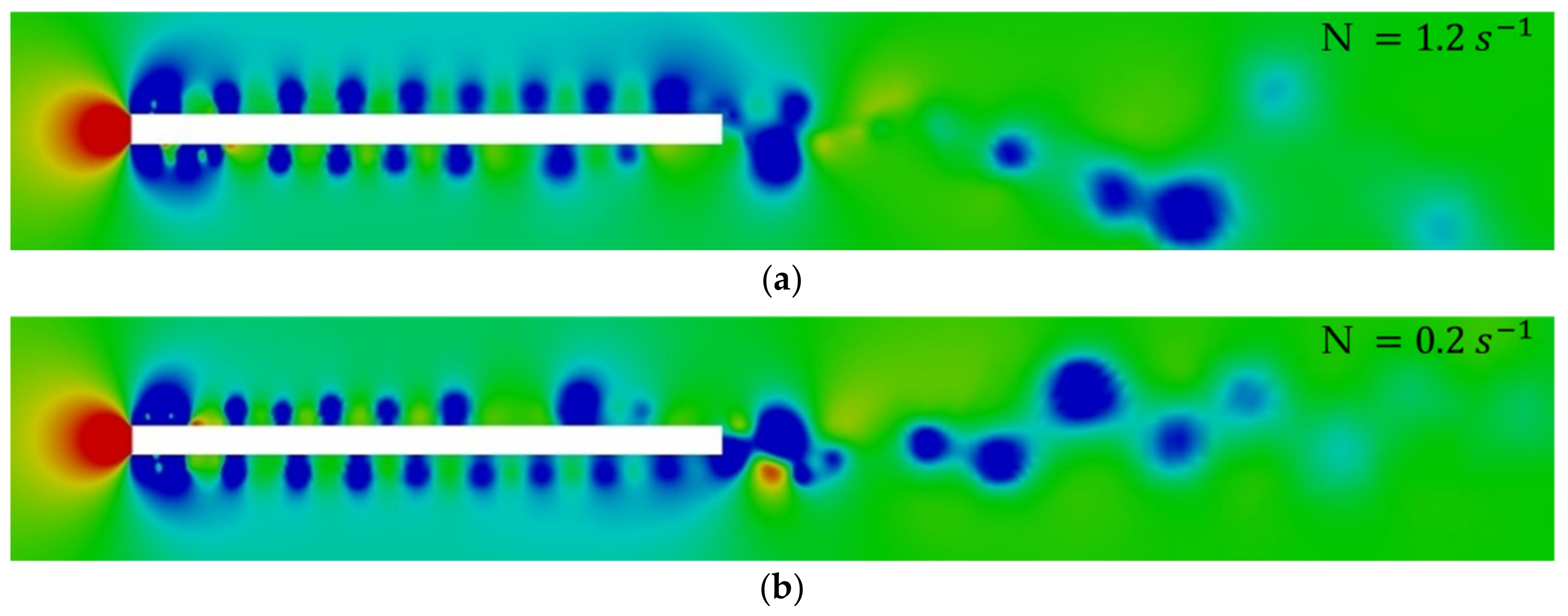
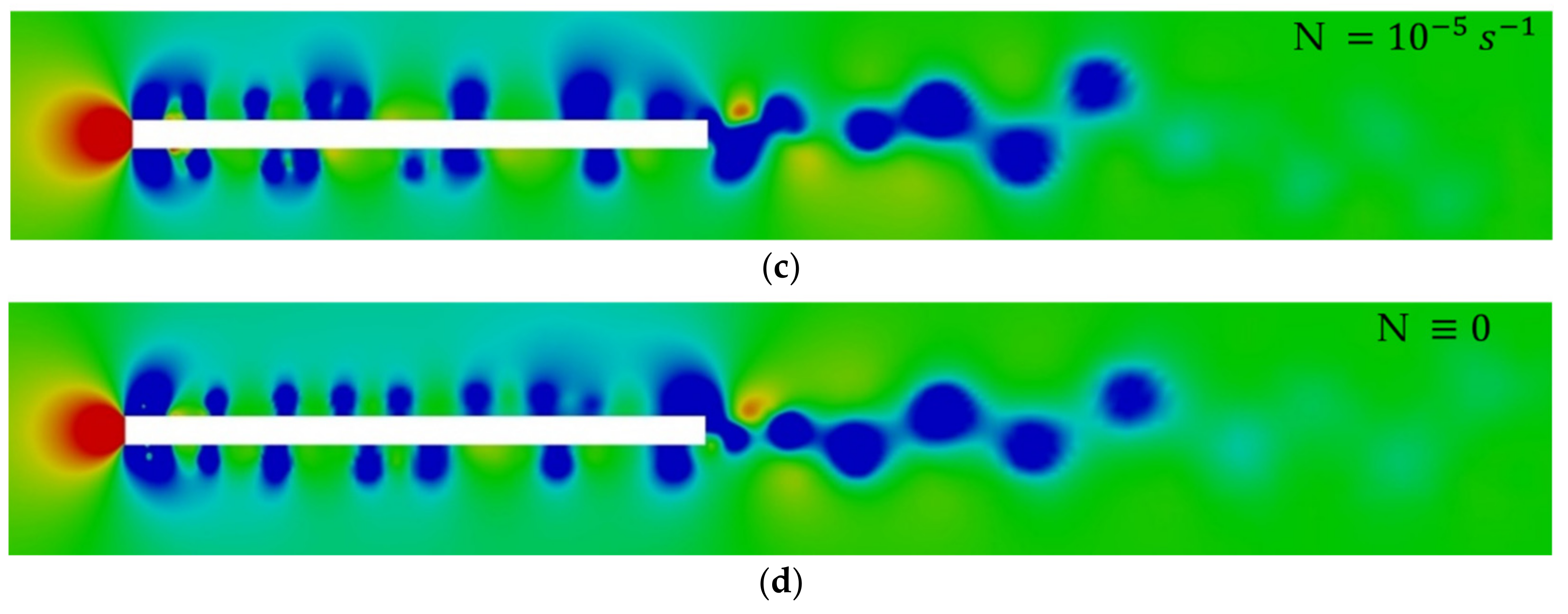
A great scientific and practical interest lies in studying the stratification effects on instantaneous flow patterns in the unsteady vortex flow regime. In the flow patterns in strongly and weakly stratified fluids, there are a number of structural flow elements, both large-scale (upstream disturbances, vortices, and internal waves) and small-scale (ligaments), which in the linear model of the flow are described by the regularly and singularly perturbed functions respectively. In the potentially homogeneous fluid, density variations are assumed infinitely small but the original mathematical formulation with the system of Equation (1) is retained, in contrast to the actually homogeneous fluid with the fundamental system degenerating on the singular components [30,31,40].

Comparison of the pressure field patterns around a horizontal plate for 4 fluid types mentioned is shown in Figure 13. Qualitatively, the flow patterns in the strongly and weakly stratified fluids are fairly similar, but there are some differences, including different positions and number of the leading-edge vortex cores, a more pronounced vortex wake in the strongly stratified fluid, etc.

A smoother boundary of the retardation flow region can be explained by influence of the buoyancy effects which damp the vertical fluid displacement. In the potentially and actually homogeneous fluids, the vortex wake is much more pronounced with a more regular form due to the absence of the collapsing influence of the stratification, as compared to the cases of the strongly and weakly stratified fluids. In general, the instantaneous pressure field patterns for a same time instant have a number of distinctive features for different fluid types considered that evidence considerable stratification effects on the unsteady processes of the flow evolution in time.

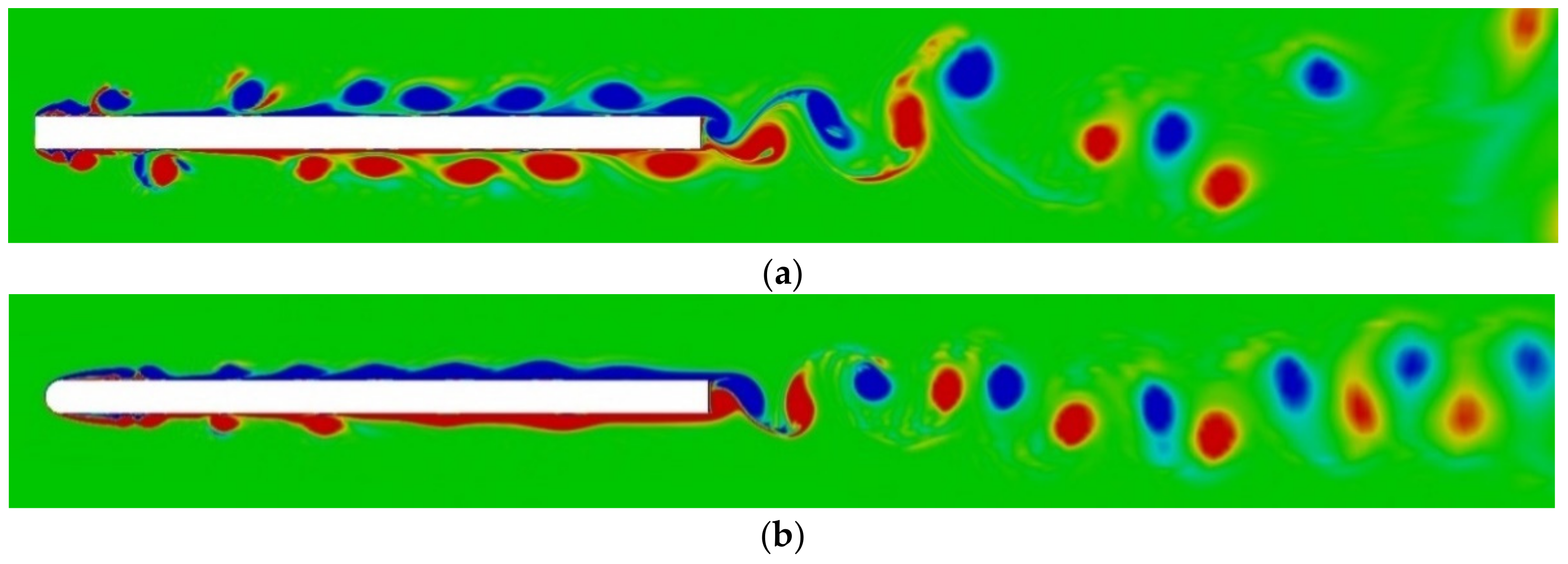
The study of the influence of the geometric shape of the leading and trailing edges of the plate on the stratified flow structure and dynamics is of a separate practical and scientific interest. This is because of the main generation of vorticity vector in the flow areas near the plate edges as a result of both the general velocity field transformation and the baroclinic effects. Figure 14 shows the stratified flow structural transformation for various designs of the plate edges, including rounding of the sharp corners of the leading edge and narrowing thickness of the plate toward the trailing edge.

Leading-edge vortices are formed in the vicinity of sharp corners of the leading edge of the rectangular plate and drift downstream along the plate surface interacting with the wake vortex street past the trailing edge. Due to a complex unsteady interaction of the two vortex systems, a new one is formed in the wake flow with the oscillation frequency being decreased approximately twice as compared to the primary one (Figure 14a).

When the leading edge is rounded, the vortices decrease in scale and intensity, taking on more blurred and elongated shapes as they move downstream. At the maximum considered radius of the leading edge rounding equal to half the plate thickness, the vortex scale is reduced about twice, as compared to the case of the plate with sharp edges, taking a form of damping wave perturbations downstream (Figure 14b).

The leading-edge vortices dissipate fairly fast without even reaching the trailing edge of the plate and thus do not significantly affect the wake flow, so that it retains the primary vortex wake structure. In the presence of narrowing of the plate towards the trailing edge, the flow structure around the obstacle does not change significantly, but in the wake flow, the volume and intensity of the vortex elements are noticeably reduced (Figure 14c,d). At the trailing edge of the plate, a narrow vortex wake is formed, which gradually expands and dissipates rather fast as moving downstream. At the same time, the regularity of the wake flow, observed in the case of the rounded edges and direct lateral sides of the plate, is lost.

5.5. Dynamic Characteristics

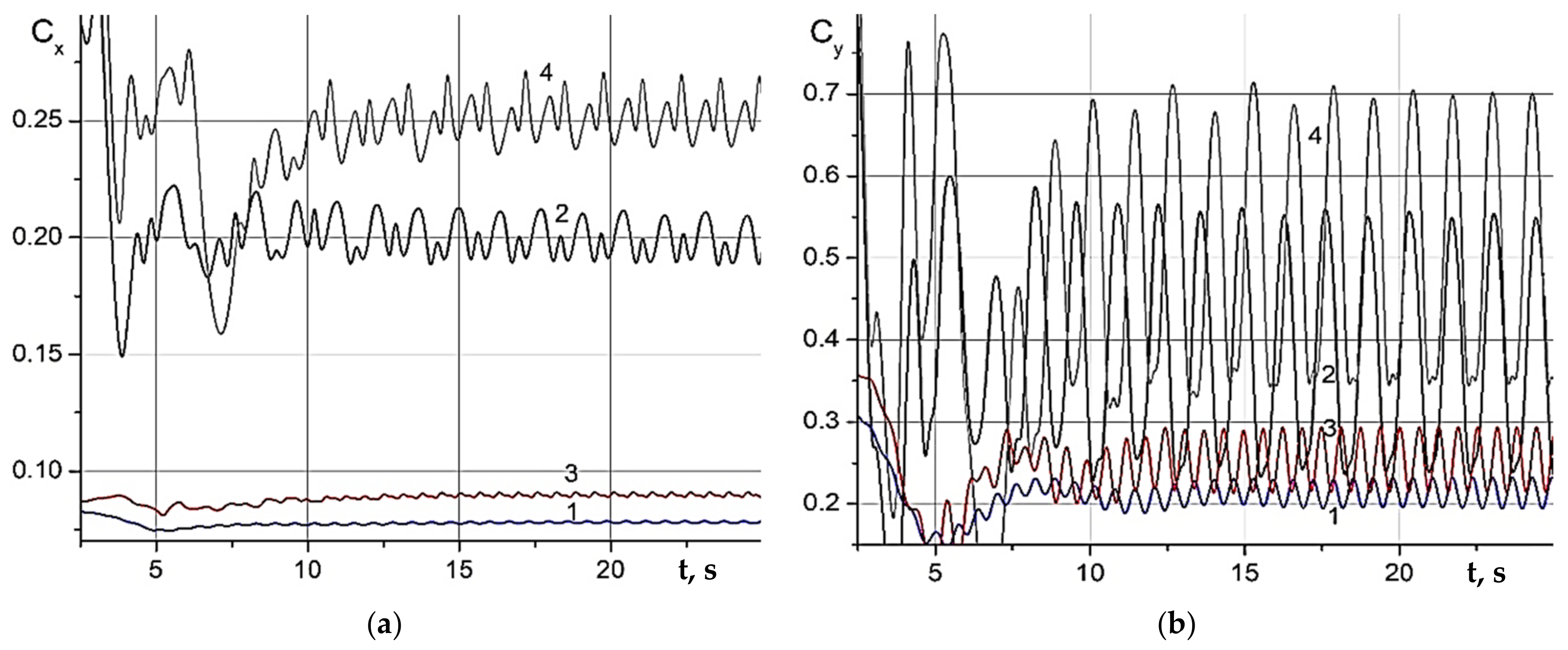
The integral values of drag and lift coefficients of the tilted plate are shown in Figure 15 as function of time, which have a substantially unsteady oscillating character in conformity with the vortex formation frequency in the wake flow past the plate. The results presented for two different values of fluid buoyancy frequency show that the vortex formation frequency slightly depends on the stratification but changes significantly with variation of tilt angle of the plate to horizon. Thus, with an almost threefold increase in the tilt angle (from α = 6° to α = 16°), the vortex formation frequency decreases approximately twice, while the oscillation amplitude increases by almost an order. In the vortex flow regime, an increase in value of the fluid stratification leads to a decrease of the integral drag due to the stratification-caused collapse of the wake vortex structures which, in this case, are a dominant flow component.

As one can see from Figure 15a, the integral drag evolution in time for α = 16° has additional lower-amplitude oscillations in antiphase to the vortex shedding ones that makes the resulting frequency of the drag oscillations almost twice greater than that for the lift.

This effect may be caused by a sort of shear layer oscillations compensating the vortex shedding ones or an instantaneous influence of mutual unsteady interactions of waves, vortices and ligaments. So far, this question remains unanswered, since requires a great deal of additional computations which cannot be carried out in an initiative unfinanced study.

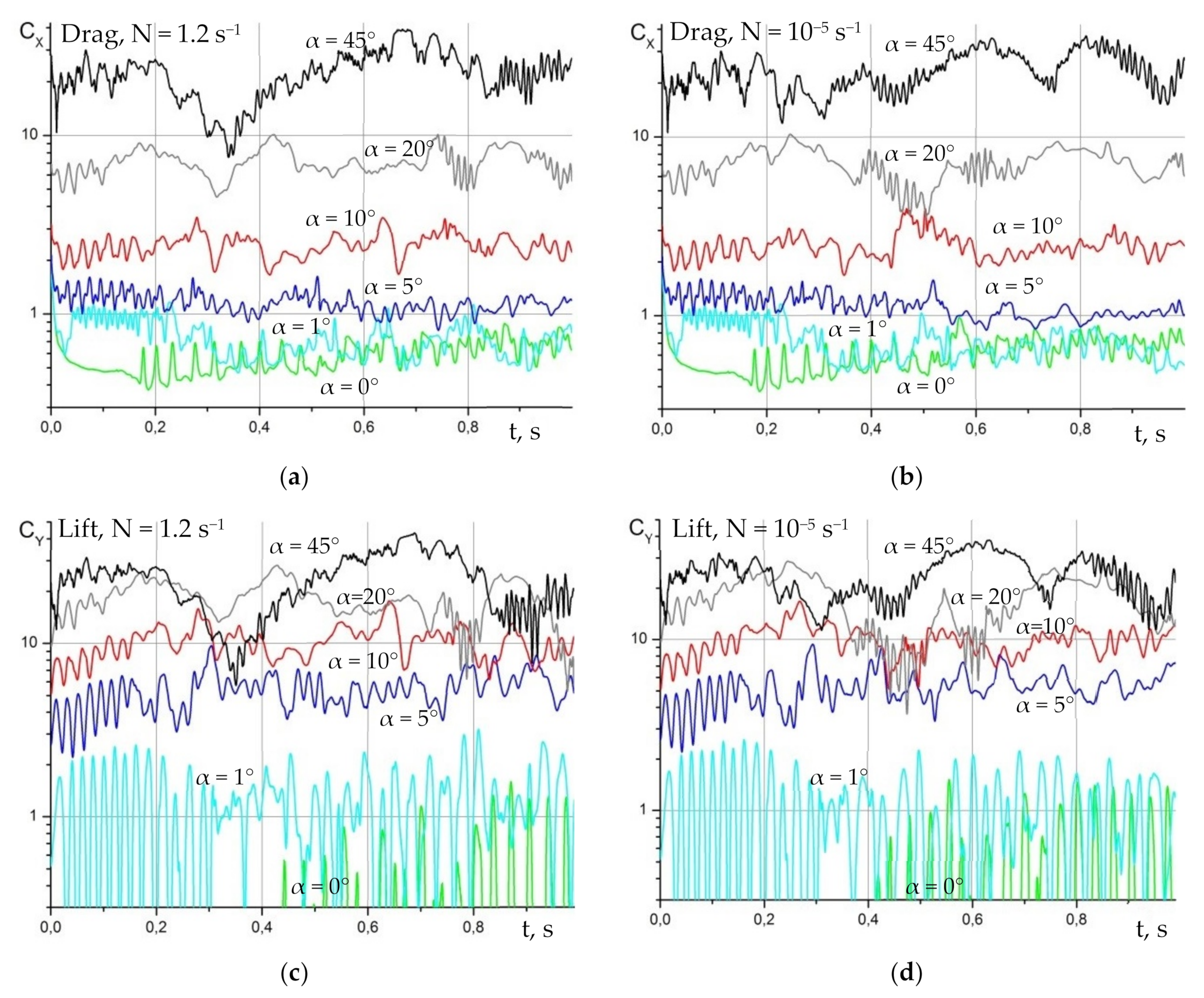
Integral values of drag and lift coefficients on a tilted plate in the strongly stratified ($N=1.2 {\mathrm{s}}^{-1}$) and potentially homogeneous fluids ($N={10}^{-5} {\mathrm{s}}^{-1}$) are shown in Figure 16 as functions of time for the case of unsteady vortex regime. All the dependencies show a complicated unsteady character, which reflects the vortex dynamics on the plate surface, and demonstrate a common feature of increase in the values of drag and lift coefficients and complication of the curves with increase in the tilt angle of the plate. The curves plotted for the different fluid types under consideration show certain differences in the unsteady character that can be explained by a noticeable stratification effect on the flow dynamics evolution for the unsteady vortex regime.

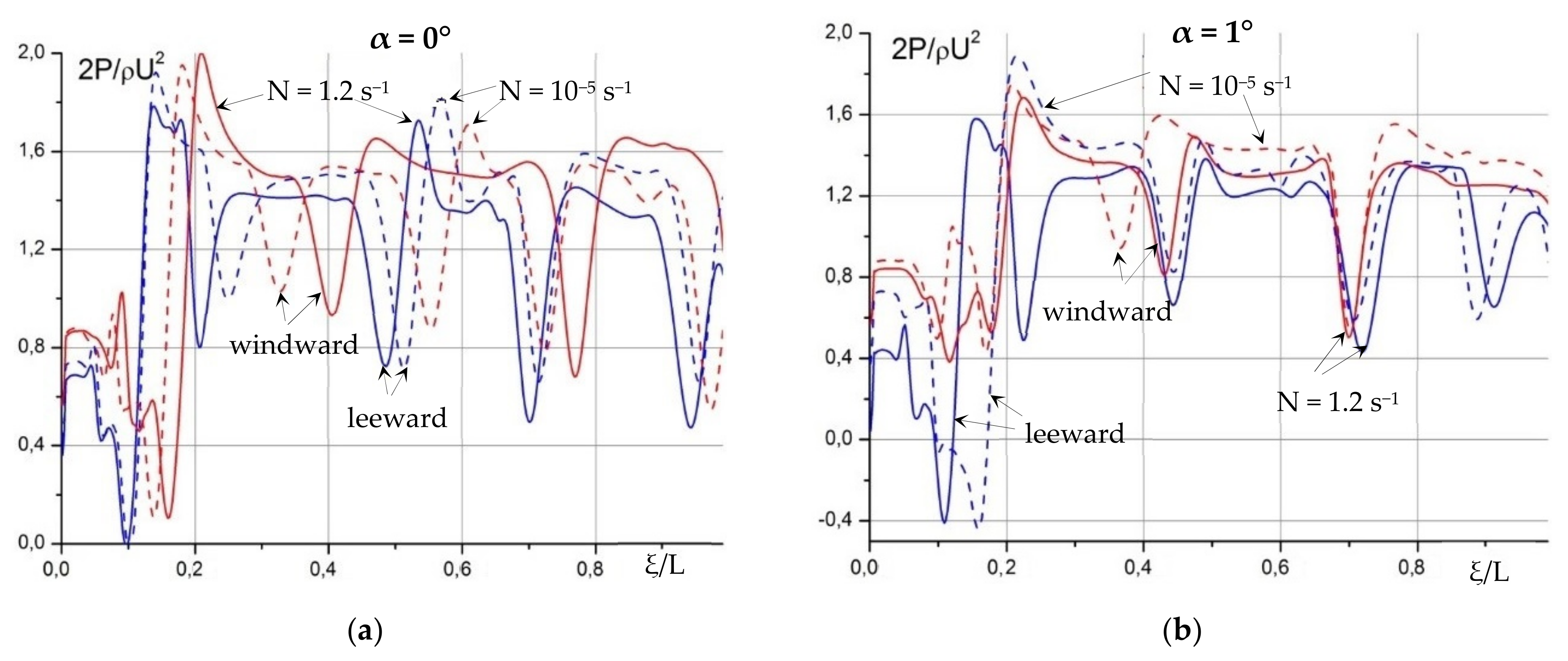
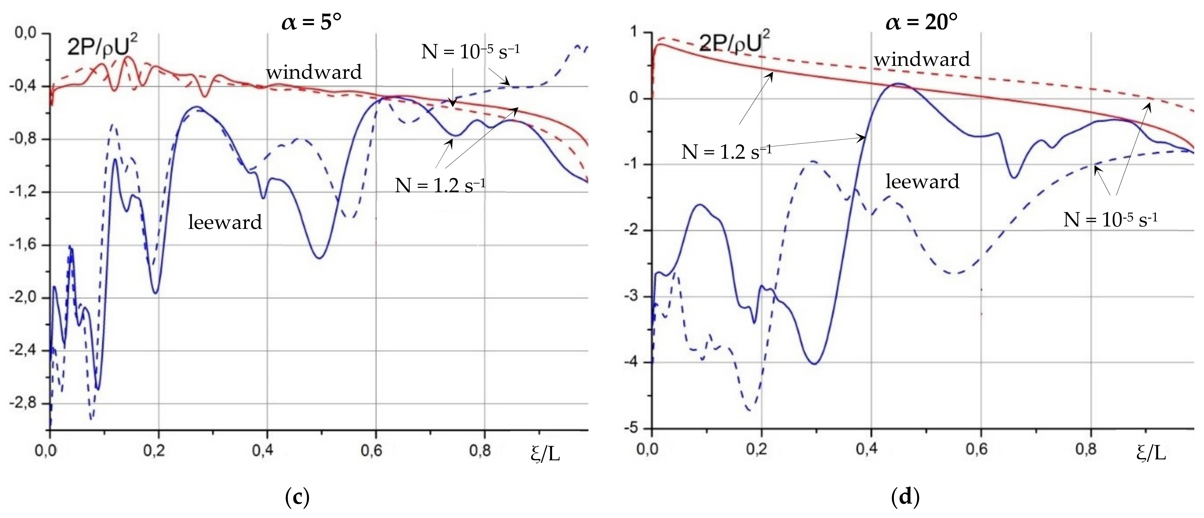
The instantaneous pressure distributions on the upper and lower sides of the plate are shown in Figure 17 for different fluid types, including strongly stratified and potentially homogeneous fluids. The structure of the distributions is essentially non-monotonic with a wavy structure and shows direct correlation with the space-time scales of the vortex perturbations. The pressure distributions on the plate surface show a strong dependence on tilt angle of the plate and fluid stratification value. At small tilt angles of the plate, the curves reflect unsteady evolution of the leading-edge vortices along the plate surface downstream. At greater tilt angles, when the leading-edge vortices start to gather in more large-scale vortex structures, the pressure distributions change their forms in correspondence with the vortex parameters. On the windward side of the plate, the pressure distributions become monotonic at $\mathsf{\alpha }>10°$, changing from a maximum value near its leading edge to a minimum at the trailing one. In general, the instantaneous pressure distributions at the same time instants for the two fluid buoyancy frequencies considered are quite different from each other that evidences considerable stratification effects on the unsteady processes of the flow evolution in time.

An interesting feature of the pressure distributions is its negative value along the whole length of the plate at $\mathsf{\alpha }=5°$ for both the windward and leeward surfaces that is not the case for the other three angles considered. This may be explained by a complicated unsteady nature of the flow at relatively high Reynolds numbers and, thus, an instantaneous influence of the continuously interacting structural flow components, such as waves, vortices, and ligaments. As the calculations show, the fields and graphs of each independent quantity, including drag and lift forces, are not similar to others due to a complex superposition of many functions.

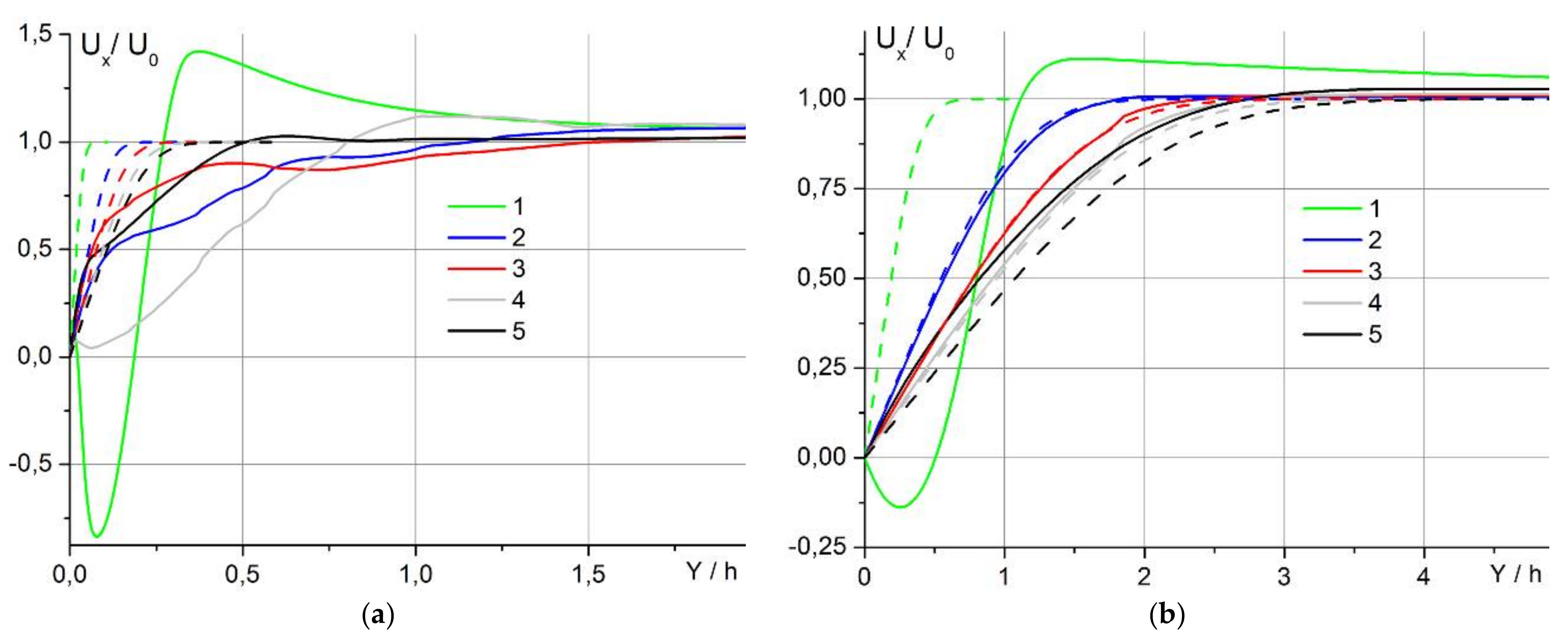
5.6. Comparison with the Blasius Solution

Instantaneous profiles of horizontal velocity component at different distances from the leading edge of a thick ($h=0.5 \mathrm{cm}$) and a thin ($h=0.05 \mathrm{cm}$) horizontal plate in the potentially homogeneous fluid are compared with the Blasius theory [8,9,10], in which the sharp edge effects and, hence, the vortex generation are not taken into account (Figure 18). Over the thin plate, the velocity profiles practically coincide with the respective curves from the Blasius solution along the whole plate length except for the regions near the plate edges, where intense processes of the fluid convergence and divergence occur. On the thick plate, the velocity profiles are essentially different from the Blasius solution due to the intense generation of leading-edge vortices.

Calculations of the integral drag coefficient on the plate surface show that its value for the thick plate ($h=0.5 \mathrm{cm}$) is 3.5 greater than that for the Blasius theory [8,9,10], but for a thin plate with thickness, $h=0.05 \mathrm{cm}$, the difference decreases to 2.3 times. It should be also mentioned that the numerical simulation of the flow over a semi-infinite plate show the difference between the numerical results and the Blasius solution less than 5%. At the same time, with a decrease in the horizontal plate thickness, the flow structure becomes less sensitive to the stratification effects due to less intensive vertical displacement of the fluid in this case.

6. Conclusions

In a single mathematical statement unsteady flow fine structure around a horizontal and a tilted plate moving in stratified or homogeneous fluids is studied numerically and visualized experimentally for different flow regimes, starting from creeping and up to unsteady vortex flow regime. The basic structural flow components, such as upstream perturbations, wake, internal waves, vortices and ligaments, are described both at the start of motion and subsequent uniform movement of the plate. The numerical and experimental results of the flow patterns around a plate are in a good agreement with each other for different flow conditions and plate parameters.

Around a motionless obstacle, fine structural diffusion-induced flows are formed in the form of multilevel vortex cells as a result of interruption of the molecular flux of a stratifying agent on the obstacle’s surface. At large times, diffusion-induced flows are mainly manifested in the form of horizontal streaky structures capable of extending over great distances from the obstacle. Around a moving body in a stratified fluid, groups of upstream perturbations, attached internal waves, leading-edge vortices, and vortex wake are formed, which coexist in the stratified flow as an organic whole being separated by fine high-gradient flow interfaces or ligaments.

Unsteady flow patterns around a plate are studied numerically and experimentally in order to determine physical mechanisms responsible for formation and evolution of the basic flow structural elements, especially, around the plate edges, i.e., in the regions with high values of pressure and density gradients. The numerical results obtained show the unsteady problem does not have a stationary limit over the entire range of flow parameters and fluid properties due to continuous mutual interactions of different flow structural elements with individual space-time scales, manifestation degree and attenuation rate.

The calculations of 2D flows performed in a unified formulation for different values of stratification are in an agreement with each other. The actually homogeneous fluid is a degenerate case due to the absence of part of the system equations and components of the complete solutions associated with them. The stratification effects, taken into account in a problem formulation, keeps its solvability for 3D case and increases the number of fine components. The solutions obtained here can be used to test newly developed programs and assess the consistency of results.

Fluid flows are a continuously evolving combination of waves, vortices, and ligaments with different scales and manifestation levels, which are in a complex spatial-temporal interaction with each other, rigid boundaries, and free stream. In order to advance in the understanding of processes and mechanisms of flow formation and evolution, additional detailed experimental and theoretical studies are required taking into account the diffusion, thermal conductivity and compressibility effects with the observability and solvability control for all the physical variables and structural components.