Abstract
The availability of reliable and efficient turbulent flow simulation methods is highly beneficial for wind energy and aerospace developments. However, existing simulation methods suffer from significant shortcomings. In particular, the most promising methods (hybrid RANS-LES methods) face divergent developments over decades, there is a significant waste of resources and opportunities. It is very likely that this development will continue as long as there is little awareness of conceptional differences of hybrid methods and their implications. The main purpose of this paper is to contribute to such clarification by identifying a basic requirement for the proper functioning of hybrid RANS-LES methods: a physically correct communication of RANS and LES modes. The state of the art of continuous eddy simulations (CES) methods (which include the required mode communication) is described and requirements for further developments are presented.
1. Introduction
Reliable and efficient turbulent flow simulation methods are an essential requirement for future wind energy and aerospace developments. Corresponding developments of simulation methods in time are illustrated in Figure 1. The striking feature is the seemingly slow progress. After developing Reynolds-averaged Navier–Stokes (RANS) equations [1,2,3,4] it became clear that this approach has significant disadvantages under conditions where it is impossible to fully explain mechanisms of turbulent flows by pure modeling (which is usually the case for wind energy and aerospace problems involving separated flow). Pure large eddy simulation (LES) methods [1,5,6,7,8], aiming at flow resolution in contrast to flow modeling, were developed as an alternative. However, it became clear that these methods result in unaffordable computational cost with respect to most wall-bounded turbulent flows of practical relevance. The conclusion was the need to develop hybrid RANS-LES [5,9,10,11,12,13,14,15], which are denoted by RANS+LES in Figure 1 (by taking reference to their conventional design strategy to combine RANS and LES equation elements). Novel hybrid RANS-LES methods, referred to as continuous eddy simulation (CES) methods, were presented recently [15,16,17,18,19]. The latter methods seem to offer major advantages regarding the serious problems of conventional hybrid RANS-LES methods and other methods [20,21,22,23].
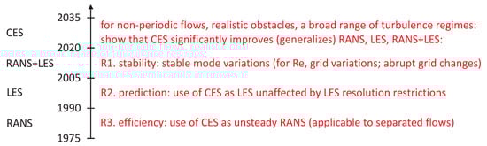
Figure 1.
An illustration of the development of computational methods for turbulent flows in time. Here, RANS+LES refers to conventional hybrid RANS-LES methods and CES refers to the CES hybrid RANS-LES methods described here. On the right-hand side (in red), there are requirements for further clarification of advantages of CES methods in relation to previously developed methods (RANS, LES, and RANS+LES).
We see diverging developments of computational methods, in particular, of hybrid RANS-LES methods over decades [15]. It is not difficult to predict that these developments will continue for a long time as long as there is little awareness of very significant differences of various hybrid methods: researchers will pick computational methods for applications according to their simplicity and availability of codes. Given the variety of available methods and model options, systematic evaluations of the suitability of using different model strategies are simply not feasible. To overcome this stagnation of the development of computational methods for turbulent flow predictions and related consequences for wind energy and aerospace applications, it needs clarification on which conceptual features are required to ensure the proper functioning of hybrid RANS-LES methods.
The latter is the main question addressed in this paper. In particular, the goal is to compare two options as illustrated in Figure 2: the option to continue with diverging developments of hybrid RANS-LES methods without paying much attention to conceptual differences, and the option to overcome conceptual problems of existing RANS-LES methods. As a basis for further discussions, typical hybrid RANS-LES methods will be described in Section 2. Then, requirements for hybrid RANS-LES methods arising from theory and applications will be pointed out in Section 3 and Section 4. Remaining challenges are described in Section 5, and conclusions will be presented in Section 6.
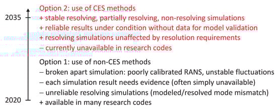
Figure 2.
In extension of Figure 1, an illustration of options regarding the future use of hybrid RANS-LES methods including characteristic advantages (+) and disadvantages (−).
2. Typical Hybrid RANS-LES Methods
Let us consider four hybrid RANS-LES models to prepare the comparison of conceptual features of CES models with three typical hybrid RANS-LES models in following sections.
Several turbulence model structures can be considered for that. Here, the model will be considered as a frame. The model is given by the incompressible continuity equation (the sum convention is used throughout this paper) and momentum equation
denotes the filtered Lagrangian time derivative. refers to the i-th component of the spatially filtered velocity. We have the filtered pressure , is the constant mass density, k is the modeled energy, is the constant kinematic viscosity, and is the rate-of-strain tensor. The modeled viscosity is given by . Here, is the modeled dissipation rate of modeled energy k, is the dissipation time scale, and is a model parameter. For k and , we consider the transport equations
The diffusion terms are given by , , and is the production of k, where is the characteristic shear rate. is a constant with standard value , and . For the RANS case considered first, the parameter where [2] implies .
One of the most popular hybrid RANS-LES models (preferred because of its original simplicity) is detached eddy simulation (DES) [13,14,24,25,26,27,28,29,30,31,32,33,34,35,36]. Reviews of DES were provided by Spalart [31] and Mockett et al. [14]. DES-type hybridizations can be applied to many turbulence model structures. Here, it is used in regard to the k equation of Equation (2),
The k equation is modified here via introducing . is a constant which is often considered to be , and refers to the filter width used in LES mode. The model switches between length scales, the RANS length scale and the LES length scale . The mechanism of switching to the LES mode is to increase the dissipation of k, leading to lower k values and a reduced modeled viscosity. The DES concept is very attractive: it is simple, also regarding its implementation, and there is only one control term that enables the simulation of resolved motions.
Different ways to hybridize the equations considered are given by partially averaged Navier–Stokes (PANS) [37,38,39,40,41,42,43,44,45], and partially integrated transport modeling (PITM) methods [20,21,22,23,46,47,48,49,50,51,52]. These methods focus on the equation in Equation (2),
where is parameterized in terms of the ratio of modeled (k) to total () kinetic energy. Within PANS, is provided by a prescribed value, whereas in PITM, is parameterized [32] involving the filter width , the total turbulence length scale (see below), and the Kolmogorov constant [1,53]. The mechanism of this approach is to reduce the dissipation of in LES mode leading to higher and a reduced modeled viscosity.
Another way of hybridizing the equations considered is given by the CES approach [15,16,17,18]. This concept implies the equations (see details given in the Appendix A)
refers to the turbulence length scale resolution ratio involving modeled (L) and total contributions (). The modeled contribution is calculated by (the brackets refer to averaging in time). The total length scale is calculated correspondingly by . Here, is the sum of modeled and resolved contributions, where the resolved contribution is calculated by . Correspondingly, is the sum of modeled and resolved contributions, , where . The functioning of this approach is similar to the functioning of PITM methods, although there is the relevant difference given by the applied. It is worth noting that CES methods can be applied in a variety of ways. It is possible to use these methods in regard to several turbulence models, and there are different ways to hybridize the equations (the hybridization can be accomplished by focusing on the k equation, as considered within the DES concept).
3. Theory Requirements: CES Versus Other Methods
Let us consider first requirements for hybrid RANS-LES from a theoretical viewpoint. The relevance of communication between modeled and resolved modes will be described in the following two paragraphs. Differences between hybrid RANS-LES concepts in this regard and related consequences will be pointed out in the following paragraphs of this section.
There are different kinds of motivation to develop hybrid RANS-LES methods, for example, the improvement of RANS predictions, or the ability to perform LES without having to deal with the resolution requirements of LES (which is very difficult for atmospheric boundary layer (ABL) simulations, where usually rather coarse grids have to be applied [54]). Arguably, the strongest motivation to develop hybrid RANS-LES is the need to predict turbulent flows of practical relevance at very high , where other prediction techniques as experiments of resolved LES are inapplicable. In this regard, the most essential requirement for hybrid models (given by requirement R1 referenced in Figure 1) is the model’s ability to stably redistribute modeled and resolved motions in response to grid and variations. The modeled motions are represented by the turbulence model applied. The resolved motions are determined by the grid applied, they are produced by the simulation equations applied. These sorts of motion need to communicate with each other. Under resolving conditions, the model contribution should be relatively small, whereas under non-resolving conditions, the model contribution has to be relatively large. The biggest challenge is that this interplay of modeled and resolved motions needs to be functional under significant grid and variations (this means the amount of modeled motion has to increase if the grid becomes coarser or becomes higher).
What is the consequence if models cannot deal with this requirement? In this case, the simulation mechanism is broken apart: there is one (in hybrid simulations usually poorly calibrated) RANS mode, and there is random resolved motion, which is often seen to be unstable because of the poor calibration of the modeled viscosity. Obviously, such methods cannot be expected to properly reflect the physics of wall-bounded turbulent flows, such methods do not have predictive power, they always need evidence for their predictions.
CES methods include such a communication mechanism, see the illustration in Figure 3. The model determines the modeled viscosity , which controls the amount of resolved motion (it needs to be sufficiently small such that fluctuations can develop). The model receives information about the amount of resolved motion via the resolution indicator . Accordingly, the model modifies its contribution to the simulation, see the illustration in Figure 3. On the other hand, most other hybrid methods (like DES or PANS described above) do not include such a communication mechanism between modeled and resolved motions, this means these methods suffer from the serious problems described in the preceding paragraph.
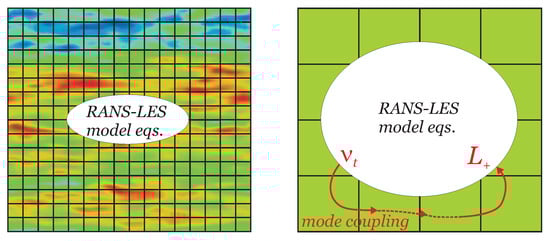
Figure 3.
An illustration of the interplay of modeled motion (indicated by ellipses of different size) and resolved motion (indicated by blue and red turbulent fluctuations). The mode coupling mechanism is illustrated by red lines on the right. The grid is illustrated by vertical and horizontal black lines. On the left, there is a case with high flow resolution, on the right there is a case with almost no flow resolution.
It is worth noting that the availability of the mode communication mechanism is not the only requirement. This mechanism needs to be designed in line with the physics of non-homogeneous turbulent flows, i.e., concepts applicable to homogeneous flows may be inapplicable to non-homogeneous flows. CES methods have this property, whereas PITM methods apply the mode communication concept for homogeneous flows. The latter implies obvious shortcomings in regard to applications to non-homogeneous flows. For example, there are discrepancies between the imposed resolution and the actual resolution seen in simulations, and resolution indicators show an unphysical behavior near walls.
The conclusion of the discussion in this section is that (in contrast to other methods) CES methods can properly deal with requirement R1 described in Figure 1. CES methods also can properly deal with the requirements R2 and R3. Resolution requirements of LES are avoided by the fact that the LES filter width is not explicitly involved, which constrains LES to the use of sufficiently fine grids. In contrast to pure RANS, the inclusion of in the equations considered enables the generation of resolved motion in RANS, which is known to be highly beneficial for separated flows.
4. Application Requirements: CES Versus Other Methods
In general, the validation of hybrid RANS-LES methods represents a daunting task given the variety of flow configurations, grid configurations, turbulence models, and hybrid versions that should be considered [15,18]. However, there are differences in this regard between conventional hybrid RANS-LES and CES methods. After addressing these differences in Section 4.1 we present in Section 4.2 and Section 4.2 CES application results and related conclusions with respect to the requirements R1–R3 described in the last paragraph of Section 3 and Figure 1.
4.1. Application Requirements: CES Versus Other Methods
Obviously, the most relevant requirement for hybrid RANS-LES methods is evidence for their proper performance in applications. With respect to conventional hybrid RANS-LES (which do not apply any mode communication), this question is usually addressed by model evaluations based on experimental or resolved LES data, often combined with the demonstration of advantages compared to RANS or under-resolved LES. Such validation studies are demanding: they need to be performed for a variety of grids (e.g., because of the known grid sensitivity of DES), and usually they involve the consideration of several flow configurations. In addition, such studies may suffer from questions about the applicability of LES and experiments used for validation for high complex flows. The basic validation concept may be seen as validation by examples (application to different flow configurations).
The validation of a hybrid RANS-LES model with ability to properly deal with the mode communication described above is different from the validation of models that do not address the mode communication due to the model’s inherent validation ingredient given by using the model in resolving mode [16]. Every hybrid simulation can be validated by using the model in resolving LES mode. This sort of validation may be seen as validation by theory, this means the concept is much more general than the validation by examples concept that needs to be used for existing approaches. Therefore, in a strict sense, model applications serve as illustrations of the proper functioning of the concept in contrast to their role regarding the evaluation of existing hybrid models: the demonstration of the model’s ability to properly work for a few benchmark cases (to deal with the requirements R1–R3 described in Figure 1) appears to be appropriate to support further model applications. In addition to the reduced number of cases that need to be considered in applications, it is worth noting that the requirements for grid sensitivity studies is also reduced for the models considered here because of the model’s inherent stability with respect to grid variations (in contrast to DES).
Based on the facts described in the preceding paragraph, we will demonstrate the proper functioning of CES methods by applications to periodic hill flows [17] compared to available LES results. Key results of such applications will be described next. Although not shown here, very similar findings were found with respect to applications of the models considered to the NASA hump flow [15,55]. A relevant conclusion obtained by these periodic hill flow investigations was the equivalence of hybrid models: as long as the same analysis is applied to a turbulence model considered, different hybrid models were found to perform equivalently. The latter will be confirmed in the following by considering three hybrid two-equation models presented in Table 1. These models can be obtained by the same analysis as used in the Appendix A.

Table 1.
Overview of CES models considered in [17]. CES-KO refers to CES performed with the model. In particular, -KOS (-KOK, -KOKU) refer to CES-KO performed by modifying the scale equation (the k equation, the turbulent time scales in the k equation according to unified RANS-LES).
4.2. Periodic Hill Flow Simulations
The CES approach described above was used to simulate periodic hill flows [17] on several grids at different Reynolds numbers in comparison to measurements of Rapp and Manhart [56], which are available for K. The Reynolds number is based on the hill height h and bulk velocity above the hill crest, which is located at . The height h and were used for the definition of non-dimensional variables presented. The flow configuration is illustrated in Figure 4, essential simulation data are given in Table 2.
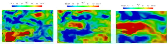
Figure 4.
Streamwise velocity fluctuations u (xz-plane, ) using the CES-KOKU model on the 500 K grid: = 37 K (left), 100 K (middle), 500 K (right).
Table 2.
Periodic hill flow simulation set-up data.
All the simulations have been performed by using the OpenFOAM CFD Toolbox [57]. The combinations of cases and grids enabled the analysis of cases where there was an almost complete resolution (as given for K using the finest 500 K grid) and a minimum of flow resolution (as given for K using the coarsest 120 K grid). Figure 5 shows the influence of variations on the 500 K grid. The case of almost complete flow resolution is on the left. The increase in implies a decreasing flow resolution, which is reflected by less details regarding the representation of instantaneous turbulent flow structures.
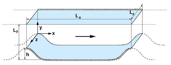
Figure 5.
The hill flow geometry.
Figure 6 addresses the suitability of three CES models presented in Table 1 with respect to the almost resolving, K (500 K grid) case. It may be seen that the flow variables , , and obtained by these models agree very well with the measurements (the measured stresses are known to be slightly under-predicted [17,58,59]). In particular, all three models perform almost equally. This observation is clearly relevant. It means that rather different models are capable to realize about the same flow resolution as long as the mode communication mechanism is set up in the same, physically correct way. The flow resolution indicators , , and , the corresponding modeled to total variables, are related to each other by . It may be seen that the assumption , which is often applied in PANS and PITM modeling approaches, represents a reasonable approximation for the well resolving case considered with the exception of the most relevant near-wall regions. It is remarkable to see the relatively uniform variation of , , and in space, showing a relatively uniform flow resolution over most of the domain. As required, and increase in the near-wall region because of the increasing amount of flow modeling (the and values indicate that the models work approximately in LES mode away from walls and in almost RANS mode close to walls). Minor differences between the three CES models considered can be observed. The latter is plausible because of the fact that different model equations are applied. However, based on the flow variable profiles we conclude that the effect of such very minor variations of resolution indicators on the actual flow simulation is negligible.
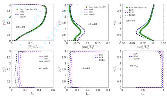
Figure 6.
Profiles of flow variables and resolution indicators obtained by periodic hill flow simulations for the K (500 K grid case) at . CES models applied are specified in the plots. The first row shows the mean velocity, streamwise normal, and Reynolds shear stress. The resolution indicators , , and are shown in the second row. Reprinted with permission from Ref. [17]. Copyright 2020 AIP Publishing.
Figure 7 addresses the core problem: the functioning of the mode communication to accomplish a proper redistribution of modeled and resolved motions. The expectation is simple: a coarser grid and a higher need to imply an increased amount of resolved motion. Reynolds number effects in consistency with Figure 5 cases are considered in the first row. The experimental data involved only apply to the K case. It may be seen that the mean streamwise velocity tends toward a more uniform spatial distribution. The plots show the essential model feature. As required, an increased leads to higher values (i.e., a decreased amount of flow resolution). The latter also applies to the near-wall region. Grid effects are considered in the second and third row. It is essential to note that grid effects have little influence on the flow simulation (again, experimental data only apply to the K case). The almost complete modeling case is involved here for K, the coarsest 120 K grid. It is remarkable that such RANS-type simulations imply mean streamwise velocity profiles that hardly differ from higher resolved cases. The plots show the required model behavior, increases (the amount of flow modeling increases) if the grid becomes coarser, as may be seen very well in the zoomed-in plots close to the upper wall.
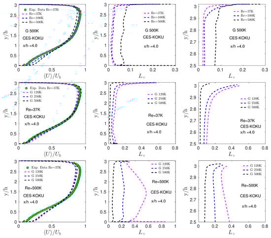
Figure 7.
Profiles of , overall and upper wall obtained by CES-KOKU simulations at . and grids applied are specified in the plots. First row: effects using the 500 K grid. Second and third row: grid effects for K. Reprinted with permission from Ref. [17]. Copyright 2020 AIP Publishing.
4.3. Summary
Based on the results presented in Section 4.2, the following conclusions can be drawn regarding the requirements R1–R3 described in Figure 1.
- R1.
- Most importantly, based on an exact solution to the problem considered [16,17,18], it is shown that the CES method can deal with the required mode balance with respect to both, significant Reynolds number and grid variations. The model performance is hardy affected by redistributions of resolved and modeled motions. The hybridization mechanism works almost equivalently for different turbulence model structures;
- R2.
- The simulations include an almost complete resolution for K (500 K grid). An excellent model performance in comparison to measurements is found. Hence, RANS-type equation can provide flow resolution without involving the LES length scale ;
- R3.
- The simulations also include the limit of almost no resolution by the K (120 K grid) case. Because of significant and stable fluctuations that do not get extinguished under such very coarse grid conditions, the model still correctly reflects the physics of flow separation.
5. Some Challenges
The theoretical and computational features of CES methods reported above are very promising. However, current computational experience is limited to the analysis of periodic hill flows reported in Section 4 and confirmation that these models also properly work for the more complex NASA hump flow [15,55] (not shown). Obviously, applications to different and in particular more complex flows would be highly beneficial to build further confidence in the ability of these hybrid methods. Although complex applications like comprehensive wind farm simulations are finally the goal, it is fair to note that applications of intermediate complexity represent a very valuable step toward wind farm simulations [60,61,62,63,64,65]. The consideration of non-periodic flows around realistic obstacles (e.g., airfoil-type simulations) involving flow separation and a broad range of turbulence regimes appears to be well appropriate to serve this purpose. Another type of equally important applications is given by the demonstration that the CES methods considered are capable of providing a basic solution for the so called Terra Incognita problem: see [19] and the references therein.
There are specific challenges in extension of the requirements R1–R3 described in Figure 1 and beyond these requirements that need to be addressed in such additional applications.
- C1.
- The core component of CES hybrid methods, the stable functioning of the mode communication mechanism, needs further investigations with respect to grid variations. Applications involving abrupt grid changes inside domains (LES-type regions embedded by RANS-type regions) are beneficial to attain a more comprehensive understanding of the stability of the generation mechanism of turbulent fluctuations. Such simulations represent the core component of atmospheric mesoscale to microscale couplings (which are closely related to the Terra Incognita problem [19]);
- C2.
- Under many circumstances LES have to be performed on relatively coarse grids, leading to the question of how well resolving the LES actually is [54]. In this regard, the use of CES methods as resolving methods is highly attractive because these methods are not constrained by strict LES resolution requirements (the use of grids which ensure that the LES filter width is smaller than typical large-scale turbulence structures). It needs specific comparisons between relatively well resolving LES and CES methods in this regard;
- C3.
- Their computational efficiency makes RANS-type simulations very attractive, for example for ABL simulations involving wind turbines. However, the inability of RANS to deal with flow separation hampers such simulations significantly. Existing periodic hill flow simulations indicate that CES used on the same grids as RANS has the potential to deal with this problem in a much more appropriate way, the question is whether the same conclusion can be drawn for more complex flows. Due to the low level of flow resolution under such conditions, it appears to be beneficial to implement a dynamic calculation of model parameters in CES methods [58,59,66,67,68,69,70], which is currently not accomplished;
- C4.
- CES methods were currently only applied to turbulent velocity fields. The extension to scalar field simulations is clearly desirable to deal, for example, with atmospheric chemistry problems. The theoretical extension of CES methods to passive scalar field simulations was presented recently in [18]. It turned out that the analysis technique applied for velocity fields is capable to also provide a corresponding hybridization of scalar field simulations (which is the same as long the ratio of turbulence and scalar time scales is constant). However, applications of these methods do not exist so far, they are required to build confidence in the treatment of scalar transport in this way;
- C5.
- The structure of CES methods applied so far corresponds to the structure of eddy viscosity type models, which are known to have deficiencies for complex turbulent flow applications. As shown in [18], it is possible to generalize such eddy viscosity type formulations to corresponding Reynolds stress transport models and even their underlying probability density function transport equations (the latter applies to both turbulent velocities and scalars). The use of eddy viscosity type methods for the periodic hill flows considered did not reveal any need for more complex turbulence models. However, there is the question of whether the same conclusion is obtained with regard to more complex flow simulations;
- C6.
- The core motivation of developing hybrid RANS-LES methods is to build the reliable capability to predict turbulent flows at very high Reynolds numbers that cannot be studied or correctly predicted otherwise. The challenge is to provide convincing evidence that the CES methods considered are able to fulfill this task. This has to be completed in comparison to usually applied hybrid RANS-LES (for example, in comparison to DES) in order to demonstrate the different capabilities of methods.
6. Conclusions
Arguably, DES and its improved versions are regularly applied for turbulent flow simulations by researchers if there is the need to use a hybrid RANS-LES method (if RANS simulations are known to fail). The basis of using DES or similar hybrid methods is the availability of DES implementations (the simplicity of its implementation) combined with the understanding that the inclusion of resolved motion is often helpful. There is, however, a price to pay for this strategy. There is a high grid dependence of DES and similar hybrid methods, which results in the need for validation data and in the need to search for the grid appropriate for the application considered. In general, the concept for justifying conventional RANS-LES (validation by examples, i.e., validation by applications to different flow configurations) is expensive and without any guarantee to produce reliable results for very high complex turbulent flows.
The reason for these serious problems of usually applied hybrid RANS-LES was identified here: it is the missing mode communication mechanism in these methods. It was also shown that CES methods do not suffer from this problem. Both theoretical features and existing applications support the suitability of this approach. Relevant advantages are given by the opportunities to perform reliable (LES-type) resolved simulations and computationally cheap RANS-type simulations that still stably involve unsteadiness, which is known to be very beneficial for separated turbulent flows simulations. With respect to routine applications there is the minor disadvantage that the mode communication needs to be implemented (via a corresponding extension of RANS codes). The very significant advantage is the stable grid dependence, which is the key for reliable predictions of complex turbulent flows at very high .
Requirements for further developments and applications of CES methods were pointed out. In regard to reliable predictions of very high complex turbulent flows (under conditions where other techniques like experiments and resolved LES are inapplicable because of their resolution requirements), there is the simple question of what would be a reasonable alternative to further developments of CES methods.
Author Contributions
Conceptualization, S.H., J.P. and B.S.; methodology, S.H.; validation, S.H.; formal analysis, S.H.; investigation, S.H., J.P. and B.S.; resources, S.H., J.P. and B.S.; writing—original draft preparation, S.H.; writing—review and editing, S.H., J.P. and B.S.; project administration, S.H., J.P. and B.S.; funding acquisition, S.H., J.P. and B.S. All authors have read and agreed to the published version of the manuscript.
Funding
This article received support of the Hanse-Wissenschaftskolleg (HWK, Delmenhorst, Germany, monitor M. Kastner) via the HWK fellowship of S.H.
Institutional Review Board Statement
Not applicable.
Informed Consent Statement
Not applicable.
Data Availability Statement
The data that support the findings of this study are available within the article.
Acknowledgments
S. Heinz would like to acknowledge support through NASA’s NRA research opportunities in aeronautics program (Grant No. NNX12AJ71A), support from the National Science Foundation (DMS-CDS&E-MSS, Grant No. 1622488), and support of the Hanse-Wissenschaftskolleg (Delmenhorst, Germany, monitor M. Kastner).
Conflicts of Interest
The authors declare no conflict of interest.
Appendix A. CES Derivation
To hybridize Equation (2), we consider a variable (instead of a constant ) combined with an appropriate calculation of . Then, we consider variations of model parameters () and related variations of model variables (like k and ): the question is which model coefficient satisfies variation equations implied by the turbulence model considered. The approach applied below follows a recently presented approach [16]. The technical framework applied to derive these results was provided by an analysis of Friess et al. [32]. The significant difference to the latter findings is that Friess et al. focused on a different question: for given PANS/PITM-type relations between model coefficients and resolution indicators, they determined equivalence criteria for hybrid methods based on other turbulence models.
By replacing P in the Equation (2) according to and taking the variation (denoted by ) of this equation we obtain the exact relation
where the Equation (2) is applied to replace . Here, we introduced the abbreviation
The coefficient calculated via Equation (A1) should not depend on or . This corresponds to the neglect of Q, i.e., . Additionally, the coefficient should not be proportional to the turbulent transport term , which does not reflect a systematic influence on the relationship between and variables characterizing the flow resolution. Thus, the second term in Equation (A1) should be equal to zero. It turns out that this is the case if we follow Friess et al. [32,71], we assume that variations of and in space can be neglected. This means we look for model coefficient variations that produce a uniform relative variation of the energy partition over the domain. In the first order of approximation, we find and . In contrast to corresponding relations reported by Friess et al. [32], these expressions include variations. Hence, the second term in Equation (A1) disappears. We find then
This relation is equivalent to
which involves . This equation can be integrated from the RANS state to a state with a certain level of resolved motion, . We obtain in this way
References
- Pope, S.B. Turbulent Flows; Cambridge University Press: Cambridge, UK, 2000. [Google Scholar]
- Wilcox, D.C. Turbulence Modeling for CFD, 2nd ed.; DCW Industries: La Cañada Flintridge, CA, USA, 1998. [Google Scholar]
- Durbin, P.A.; Petterson, B.A. Statistical Theory and Modeling for Turbulent Flows; John Wiley and Sons: Hoboken, NJ, USA, 2001. [Google Scholar]
- Hanjalić, K. Advanced turbulence closure models: A view of current status and future prospects. Int. J. Heat Fluid Flow 1994, 15, 178–203. [Google Scholar] [CrossRef]
- Sagaut, P. Large Eddy Simulation for Incompressible Flows: An Introduction; Springer: Berlin/Heidelberg, Germany, 2002. [Google Scholar]
- Lesieur, M.; Metais, O.; Comte, P. Large-Eddy Simulations of Turbulence; Cambridge University Press: Cambridge, UK, 2005. [Google Scholar]
- Piomelli, U. Large-eddy simulation: Achievements and challenges. Prog. Aerosp. Sci. 1999, 35, 335–362. [Google Scholar] [CrossRef]
- Meneveau, C.; Katz, J. Scale-invariance and turbulence models for large-eddy simulation. Annu. Rev. Fluid Mech. 2000, 32, 1–32. [Google Scholar] [CrossRef]
- Speziale, C.G. Turbulence modeling for time-dependent RANS and VLES: A review. AIAA J. 1998, 36, 173–184. [Google Scholar] [CrossRef]
- Germano, M. Properties of the hybrid RANS/LES filter. Theor. Comput. Fluid Dyn. 2004, 17, 225–231. [Google Scholar] [CrossRef]
- Hanjalić, K. Will RANS survive LES? A view of perspectives. ASME J. Fluids Eng. 2005, 127, 831–839. [Google Scholar] [CrossRef]
- Fröhlich, J.; Terzi, D.V. Hybrid LES/RANS methods for the simulation of turbulent flows. Prog. Aerosp. Sci. 2008, 44, 349–377. [Google Scholar] [CrossRef]
- Chaouat, B. The state of the art of hybrid RANS/LES modeling for the simulation of turbulent flows. Flow Turbul. Combust. 2017, 99, 279–327. [Google Scholar] [CrossRef] [Green Version]
- Mockett, C.; Fuchs, M.; Thiele, F. Progress in DES for wall-modelled LES of complex internal flows. Comput. Fluids 2012, 65, 44–55. [Google Scholar] [CrossRef]
- Heinz, S. A review of hybrid RANS-LES methods for turbulent flows: Concepts and applications. Prog. Aerosp. Sci. 2020, 114, 100597/1–100597/25. [Google Scholar] [CrossRef]
- Heinz, S. The large eddy simulation capability of Reynolds-averaged Navier-Stokes equations: Analytical results. Phys. Fluids 2019, 31, 021702/1–021702/6. [Google Scholar] [CrossRef]
- Heinz, S.; Mokhtarpoor, R.; Stoellinger, M.K. Theory-based Reynolds-Averaged Navier-Stokes equations with Large Eddy Simulation capability for separated turbulent flow simulations. Phys. Fluids 2020, 32, 065102/1–065102/20. [Google Scholar] [CrossRef]
- Heinz, S. The Continuous Eddy Simulation capability of velocity and scalar Probability Density Function equations for turbulent flows. Phys. Fluids 2021, 33, 025107/1–025107/13. [Google Scholar] [CrossRef]
- Heinz, S. Theory-based mesoscale to microscale coupling for wind energy applications. Appl. Math. Model. 2021, 98, 563–575. [Google Scholar] [CrossRef]
- Schiestel, R.; Dejoan, A. Towards a new partially integrated transport model for coarse grid and unsteady turbulent flow simulations. Theor. Comput. Fluid Dyn. 2005, 18, 443–468. [Google Scholar] [CrossRef]
- Chaouat, B.; Schiestel, R. A new partially integrated transport model for subgrid-scale stresses and dissipation rate for turbulent developing flows. Phys. Fluids 2005, 17, 065106/1–065106/19. [Google Scholar] [CrossRef]
- Chaouat, B.; Schiestel, R. Analytical insights into the partially integrated transport modeling method for hybrid Reynolds averaged Navier-Stokes equations-large eddy simulations of turbulent flows. Phys. Fluids 2012, 24, 085106/1–085106/34. [Google Scholar] [CrossRef]
- Chaouat, B.; Schiestel, R. Hybrid RANS-LES simulations of the turbulent flow over periodic hills at high Reynolds number using the PITM method. Comput. Fluids 2013, 84, 279–300. [Google Scholar] [CrossRef]
- Spalart, P.R.; Jou, W.H.; Strelets, M.; Allmaras, S.R. Comments on the feasibility of LES for wings, and on a hybrid RANS/LES approach. In Advances in DNS/LES; Liu, C., Liu, Z., Eds.; Greyden Press: Dayton, OH, USA, 1997; pp. 137–147. [Google Scholar]
- Travin, A.; Shur, M.L.; Strelets, M.; Spalart, P. Detached-eddy simulations past a circular cylinder. Flow Turbul. Combust. 1999, 63, 113–138. [Google Scholar]
- Spalart, P.R. Strategies for turbulence modelling and simulations. Int. J. Heat Fluid Flow 2000, 21, 252–263. [Google Scholar] [CrossRef]
- Travin, A.; Shur, M.L. Physical and numerical upgrades in the detached-eddy simulation of complex turbulent flows. In Advances in LES of Complex Flows; Friedrich, R., Rodi, W., Eds.; Springer: Dordrecht, The Netherlands, 2002; pp. 239–254. [Google Scholar]
- Menter, F.R.; Kuntz, M.; Langtry, R. Ten years of industrial experience with SST turbulence model. Turb. Heat Mass Transf. 2003, 4, 625–632. [Google Scholar]
- Spalart, P.R.; Deck, S.; Shur, M.L.; Squires, K.D.; Strelets, M.K.; Travin, A. A new version of detached-eddy simulation, resistant to ambiguous grid densities. Theor. Comput. Fluid Dyn. 2006, 20, 181–195. [Google Scholar] [CrossRef]
- Shur, M.L.; Spalart, P.R.; Strelets, M.K.; Travin, A. A hybrid RANS-LES approach with delayed-DES and wall-modelled LES capabilities. Int. J. Heat Fluid Flow 2008, 29, 1638–1649. [Google Scholar] [CrossRef]
- Spalart, P.R. Detached-eddy simulation. Annu. Rev. Fluid Mech. 2009, 41, 181–202. [Google Scholar] [CrossRef]
- Friess, C.; Manceau, R.; Gatski, T.B. Toward an equivalence criterion for hybrid RANS/LES methods. Comput. Fluids 2015, 122, 233–246. [Google Scholar] [CrossRef] [Green Version]
- Yin, Z.; Reddy, K.R.; Durbin, P.A. On the dynamic computation of the model constant in delayed detached eddy simulation. Phys. Fluids 2015, 27, 025105/1–025105/15. [Google Scholar] [CrossRef] [Green Version]
- Rahimi, H.; Dose, B.; Stoevesandt, B.; Peinke, J. Investigation of the validity of BEM for simulation of wind turbines in complex load cases and comparison with experiment and CFD. J. Phys. Conf. Ser. 2016, 749, 012015. [Google Scholar] [CrossRef] [Green Version]
- Rahimi, H.; Dose, B.; Herraez, I.; Peinke, J.; Stoevesandt, B. DDES and URANS comparison of the NREL phase-VI wind turbine at deep stall. In Proceedings of the 34th AIAA Applied Aerodynamics Conference, Washington, DC, USA, 13–17 June 2016; AIAA Paper 16-3127. pp. 1–14. [Google Scholar]
- Sedano, C.A.; Berger, F.; Rahimi, H.; Lopez Mejia, O.D.; Kühn, M.; Stoevesandt, B. CFD validation of a model wind turbine by means of improved and delayed detached eddy simulation in OpenFOAM. Energies 2019, 12, 1306. [Google Scholar] [CrossRef] [Green Version]
- Girimaji, S. Partially-averaged Navier-Stokes method for turbulence: A Reynolds-averaged Navier-Stokes to direct numerical simulation bridging method. ASME J. Appl. Mech. 2006, 73, 413–421. [Google Scholar] [CrossRef]
- Girimaji, S.; Jeong, E.; Srinivasan, R. Partially averaged Navier-Stokes method for turbulence: Fixed point analysis and comparisons with unsteady partially averaged Navier-Stokes. ASME J. Appl. Mech. 2006, 73, 422–429. [Google Scholar] [CrossRef]
- Lakshmipathy, S.; Girimaji, S.S. Extension of Boussinesq turbulence constitutive relation for bridging methods. J. Turbul. 2007, 8, N31. [Google Scholar] [CrossRef]
- Frendi, A.; Tosh, A.; Girimaji, S. Flow past a backward-facing step: Comparison of PANS, DES and URANS results with experiments. Int. J. Comput. Methods Eng. Sci. Mech. 2007, 8, 23–38. [Google Scholar] [CrossRef]
- Lakshmipathy, S.; Girimaji, S.S. Partially averaged Navier-Stokes (PANS) method for turbulence simulations: Flow past a circular cylinder. ASME J. Fluids Eng. 2010, 132, 121202/1–121202/9. [Google Scholar] [CrossRef]
- Jeong, E.; Girimaji, S.S. Partially averaged Navier–Stokes (PANS) method for turbulence simulations: Flow past a square cylinder. ASME J. Fluids Eng. 2010, 132, 121203/1–121203/11. [Google Scholar] [CrossRef]
- Basara, B.; Krajnovic, S.; Girimaji, S.S.; Pavlovic, Z. Near-wall formulation of the partially averaged Navier-Stokes turbulence model. AIAA J. 2011, 42, 2627–2636. [Google Scholar] [CrossRef]
- Krajnovic, S.; Lárusson, R.; Basara, B. Superiority of PANS compared to LES in predicting a rudimentary landing gear flow with affordable meshes. Int. J. Heat Fluid Flow 2012, 37, 109–122. [Google Scholar] [CrossRef]
- Foroutan, H.; Yavuzkurt, S. A partially averaged Navier Stokes model for the simulation of turbulent swirling flow with vortex breakdown. Int. J. Heat Fluid Flow 2014, 50, 402–416. [Google Scholar] [CrossRef] [Green Version]
- Chaouat, B.; Schiestel, R. From single-scale turbulence models to multiple-scale and subgrid-scale models by Fourier transform. Theor. Comput. Fluid Dyn. 2007, 21, 201–229. [Google Scholar] [CrossRef]
- Befeno, I.; Schiestel, R. Non-equilibrium mixing of turbulence scales using a continuous hybrid RANS/LES approach: Application to the shearless mixing layer. Flow Turbul. Combust. 2007, 78, 129–151. [Google Scholar] [CrossRef]
- Chaouat, B.; Schiestel, R. Progress in subgrid-scale transport modelling for continuous hybrid nonzonal RANS/LES simulations. Int. J. Heat Fluid Flow 2009, 30, 602–616. [Google Scholar] [CrossRef]
- Chaouat, B. Subfilter-scale transport model for hybrid RANS/LES simulations applied to a complex bounded flow. J. Turbul. 2010, 11, N51. [Google Scholar] [CrossRef]
- Chaouat, B. Simulation of turbulent rotating flows using a subfilter scale stress model derived from the partially integrated transport modeling method. Phys. Fluids 2012, 24, 045108/1–045108/35. [Google Scholar] [CrossRef]
- Chaouat, B.; Schiestel, R. Partially integrated transport modeling method for turbulence simulation with variable filters. Phys. Fluids 2013, 25, 125102/1–125102/39. [Google Scholar] [CrossRef]
- Chaouat, B. Application of the PITM method using inlet synthetic turbulence generation for the simulation of the turbulent flow in a small axisymmetric contraction. Flow Turbul. Combust. 2017, 98, 987–1024. [Google Scholar] [CrossRef]
- Heinz, S. On the Kolmogorov constant in stochastic turbulence models. Phys. Fluids 2002, 14, 4095–4098. [Google Scholar] [CrossRef] [Green Version]
- Wurps, H.; Steinfeld, G.; Heinz, S. Grid-resolution requirements for large-eddy simulations of the atmospheric boundary layer. Bound. Layer Meteorol. 2020, 175, 119–201. [Google Scholar] [CrossRef] [Green Version]
- Greenblatt, D.; Paschal, K.B.; Yao, C.S.; Harris, J.; Schaeffler, N.N.W.; Washburn, A.E. Experimental investigation of separation control—Part 1: Baseline and steady suction. AIAA J. 2006, 44, 2820–2830. [Google Scholar] [CrossRef]
- Rapp, C.; Manhart, M. Flow over periodic hills—An experimental study. Exp. Fluids 2011, 51, 247–269. [Google Scholar] [CrossRef]
- Openfoam, the Open Source CFD Toolbox. Available online: http://www.openfoam.com (accessed on 24 November 2019).
- Mokhtarpoor, R.; Heinz, S.; Stoellinger, M. Dynamic unified RANS-LES simulations of high Reynolds number separated flows. Phys. Fluids 2016, 28, 095101/1–095101/36. [Google Scholar] [CrossRef] [Green Version]
- Mokhtarpoor, R.; Heinz, S. Dynamic large eddy simulation: Stability via realizability. Phys. Fluids 2017, 29, 105104/1–105104/22. [Google Scholar] [CrossRef] [Green Version]
- Rahimi, H.; Medjroubi, W.; Stoevesandt, B.; Peinke, J. 2D numerical investigation of the laminar and turbulent flow over different airfoils using Openfoam. J. Phys. Conf. Ser. 2014, 555, 012070. [Google Scholar] [CrossRef] [Green Version]
- Herráez, I.; Medjroubi, W.; Stoevesandt, B.; Peinke, J. Aerodynamic simulation of the MEXICO rotor. J. Phys. Conf. Ser. 2014, 555, 012051. [Google Scholar] [CrossRef] [Green Version]
- Herráez, I.; Akay, B.; van Bussel, G.J.W.; Peinke, J.; Stoevesandt, B. Detailed analysis of the blade root flow of a horizontal axis wind turbine. Wind Energy Sci. 2016, 1, 89–100. [Google Scholar] [CrossRef] [Green Version]
- Schramm, M.; Rahimi, H.; Stoevesandt, B.; Tangager, K. The influence of eroded blades on wind turbine performance using numerical simulations. Energies 2017, 10, 1420. [Google Scholar] [CrossRef] [Green Version]
- Tang, X.; Zhao, S.; Fan, B.; Peinke, J.; Stoevesandt, B. Micro-scale wind resource assessment in complex terrain based on CFD coupled measurement from multiple masts. Appl. Energy 2019, 238, 806–815. [Google Scholar] [CrossRef]
- Tafur, B.S.B.; Daniele, E.; Stoevesandt, B.; Thomas, P. On the calibration of rotational augmentation models for wind turbine load estimation by means of CFD simulations. Acta Mech. Sin. 2020, 36, 306–319. [Google Scholar]
- Heinz, S. Realizability of dynamic subgrid-scale stress models via stochastic analysis. Monte Carlo Methods Appl. 2008, 14, 311–329. [Google Scholar] [CrossRef]
- Ahmadi, G.; Kassem, H.; Peinke, J.; Heinz, S. Dynamic Large Eddy Simulation: Benefits of honoring realizability. In Proceedings of the Eleventh International Symposium on Turbulence and Shear Flow Phenomena (TSFP11), Southampton, UK, 30 July–2 August 2019; TSFP Paper 2019-P-9. pp. 1–6. [Google Scholar]
- Ahmadi, G.; Kassem, H.; Stoevesandt, B.; Peinke, J.; Heinz, S. Wall bounded turbulent flows up to high Reynolds numbers: LES resolution assessment. In Proceedings of the AIAA Aerospace Sciences Meeting, AIAA SciTech Forum, San Diego, CA, USA, 7–11 January 2019; AIAA Paper 19-1887. pp. 1–17. [Google Scholar]
- Ahmadi, G.; Kassem, H.; Mokhtarpoor, R.; Stoevesandt, B.; Peinke, J.; Heinz, S. Realizable dynamic LES of high Reynolds number turbulent wall bounded flows. In Proceedings of the AIAA Aerospace Sciences Meeting, AIAA SciTech Forum, San Diego, CA, USA, 7–11 January 2019; AIAA Paper 19-2140. pp. 1–19. [Google Scholar]
- Ahmadi, G. Dynamic Large Eddy Simulation in High Reynolds Numbers Based on Realizable Stochastic Turbulence Modeling. Ph.D. Thesis, Carl von Ossietzky Universität Oldenburg, Oldenburg, Germany, 2021. [Google Scholar]
- Manceau, R.; Gatski, T.B.; Friess, C. Recent progress in hybrid temporal-LES/RANS Modeling. In Proceedings of the V. European Conference on Computational Fluid Dynamics, ECCOMAS CFD 2010, Lisbon, Portugal, 14–17 June 2010; pp. 1–20. [Google Scholar]
Publisher’s Note: MDPI stays neutral with regard to jurisdictional claims in published maps and institutional affiliations. |
© 2021 by the authors. Licensee MDPI, Basel, Switzerland. This article is an open access article distributed under the terms and conditions of the Creative Commons Attribution (CC BY) license (https://creativecommons.org/licenses/by/4.0/).