1. Introduction
Marangoni convection is a type of non-equilibrium process, which creates a variety of spatiotemporal periodic patterns, see [
1,
2], and is crucial in thin liquid layers, where the interfacial effects prevail over the bulk effects. The formation of large-scale convective patterns is a result of long-wavelength instability.
There are two kinds of longwave Marangoni instability, (i) at small Biot number with temperature as the active, slowly evolving, variable [
3], and (ii) at moderate Galileo number with surface deformation as the active variable [
4]. The recent research of Shklyaev et al. [
5], shows that in the interval of wave numbers
(
is the Biot number defined later), both those variables are active. In that interval, large-scale monotonic and oscillatory instability modes exist, which produce stationary patterns and wave patterns, correspondingly [
6].
It is known that when the free surface of the liquid is covered by surface-active agent (surfactant), the formation of the convective patterns significantly changes. The basic experiments describing this effect can be found in [
7,
8], theoretically the behavior of large-scale patterns under the influence of adsorbed insoluble surfactant is considered in [
9]. When the surfactant is added, the linear stability boundaries, the types of bifurcation and selected patterns depend on the elasticity number and on the Biot number, see [
10].
In the present work we investigate the large-scale Marangoni convection in a liquid layer with insoluble surfactant spread over a deformable free surface, in the interval of wavenumbers
. We carry out a weakly nonlinear analysis of patterns on a square lattice in the Fourier space, which include rolls and squares. We consider the modulation of rolls by long-wave disturbances near the instability threshold and derive the system of the amplitude equations. The periodic patterns can be unstable with respect to a spatial modulation that breaks the spatial periodicity. The modulation of convective patterns in the neighborhood of the instability threshold is explained by Newell, Whitehead, and Segel [
11,
12] as interaction of disturbances with different wavenumbers close to the critical one. In the case of stationary rolls, which are chosen for the investigation in our paper, the asymptotic multiscale analysis leads to the Ginzburg-Landau equation with real coefficients. However, in the presence of slowly decaying longwave modes related to the conservation laws, that equation turns out to be insufficient. In [
13] it was shown that interaction with such a mode can significantly influence the stability of patterns. In the problem under consideration, there are two conservation laws, the conservation of the liquid volume and the conservation of the total amount of the surfactant. The corresponding modification of the stability properties of rolls is considered in the present paper. The analysis of that phenomenon has not been previously carried out for Marangoni patterns in the presence of a surfactant.
2. Statement of the Problem
We consider an infinite horizontal layer with a mean thickness , thermal diffusivity , kinematic viscosity , density , dynamic viscosity , and thermal conductivity . The layer is confined between a rigid substrate and deformable free upper boundary. The vertical axis is directed upward. The layer is heated from below with transverse temperature gradient At the upper surface the insoluble surfactant is absorbed. It is convected by interfacial velocity field and diffuses over the interface but not into the bulk. is the reference value of the surfactant concentration. The surface tension is a linear function of temperature and surfactant concentration, i.e., ( is the reference value of surface tension, ).
In [
10] we derived the system of long-wave nondimensional amplitude equations for the local film thickness
, the surfactant concentration
and perturbation of the temperature disturbance
:
Here
is the pressure disturbance and
is the temperature distribution at the free surface,
and
are horizontal coordinates and time is rescaled as
This rescaling of coordinates leads to the rescaling of the wavenumber, . The parameter is a ratio between the mean thickness and typical horizontal scale of disturbances.
The problem includes the following dimensionless parameters: is the Marangoni number, is the elasticity number, is the Lewis number ( is the surfactant diffusivity), is the Galileo number ( is the acceleration due to gravity), is the inverse capillary number, is the Biot number ( is the heat transfer coefficient). Here we assume and
The linear stability analysis of the motionless state was performed in [
10]. There are two instability modes: the monotonic one and the oscillatory one. The instability boundaries are determined by Equation (5) in [
10] for the growth rate
in the form:
For the monotonic mode the neutral stability curve is described by the formula
The critical wave number that corresponds to the minimum of the marginal stability curve of the monotonic mode does not depend on the surfactant parameters and equals the value determined in [
5]:
The threshold value of Marangoni number for the oscillatory mode was also found in our previous work [
10]. Shklyaev et al. in [
5] show that without surfactant (
) the oscillatory instability mode appears for sufficiently large values of
in a limited range of wave numbers. The oscillatory mode is critical under conditions
and
In order to analyze the competition between instability modes, we use the following property of the oscillatory instability: its appearance changes the meaning of the neutral curve (5). If there is no oscillatory instability, the Equation (5) indeed determines the monotonic instability boundary:
at
and
at
, therefore
. However, if there exists an oscillatory instability with the instability boundary
, Equation (5) determines the stabilization boundary for one of the two unstable monotonic modes, thus
(see Figure 5.1 (b) in [
14]).
Differentiating (4) with respect to
, we find that at the critical value of monotonic Marangoni number
where
One can show that even if the oscillatory instability is absent at , it can appear for , where the value of the elasticity number is determined by the relation .
Without loss of generality we can fix the value of the inverse capillary number equal to unity, i.e.,
, which corresponds to the choice
. While the elasticity number,
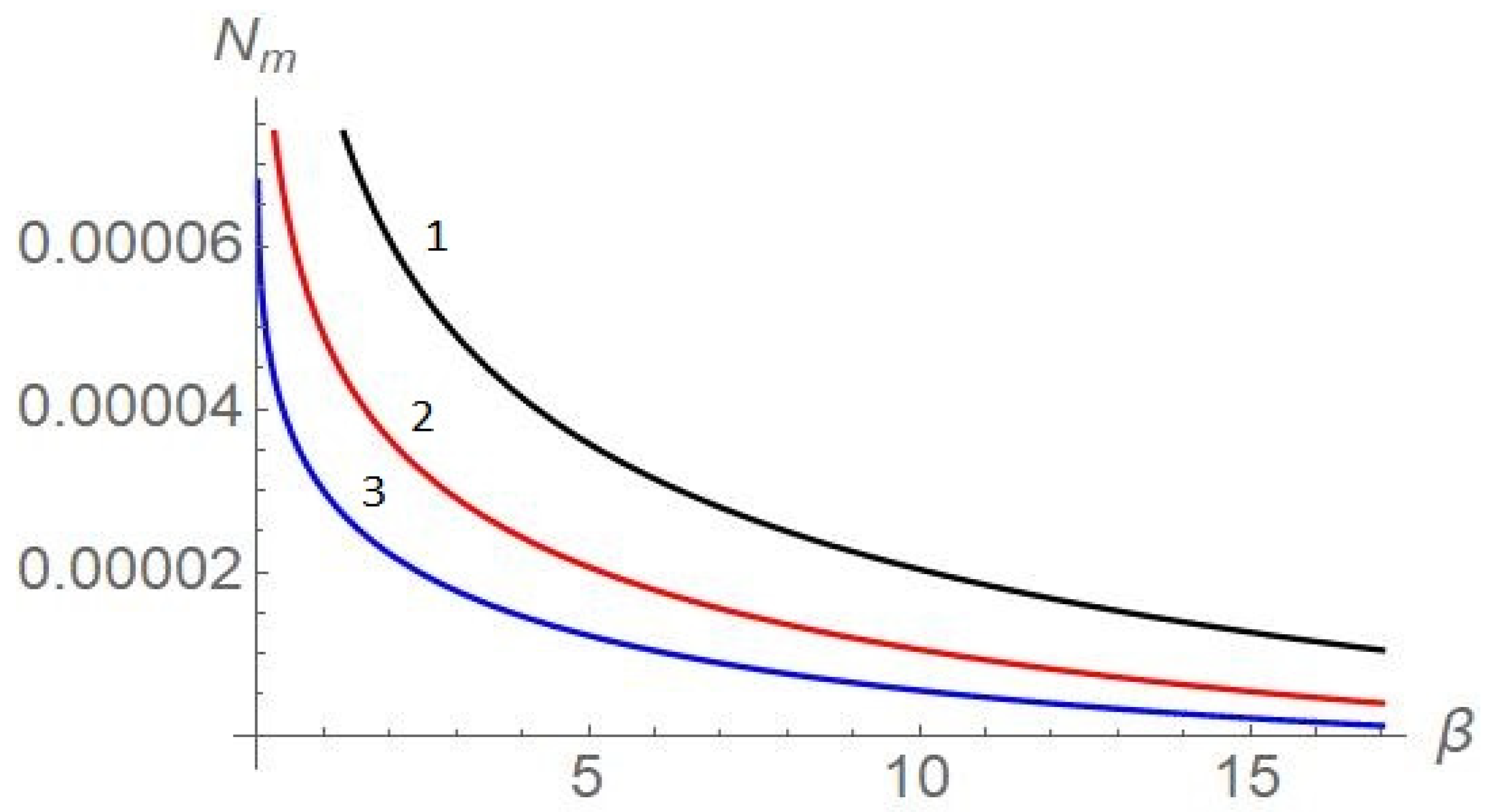
, can vary in a relatively large interval, the value of the surfactant Lewis number, which is the ratio of mass diffusivity to thermal diffusivity, has significant limitation. As an example of insoluble surfactant we consider
produced by Nikko Chemical Co. (Tokyo, Japan), for its properties see [
15,
16]. For our calculation in this paper the Lewis number is taken equal to
. The value of the wave number is taken equal to
. Then we obtain
as a function on parameters
and
, see
Figure 1. For
the critical Marangoni number
is a threshold of the monotonic instability of the equilibrium state.
3. Weakly Nonlinear Analysis of Monotonic Mode
We study the nonlinear dynamics of perturbations in the neighborhood of , ( is a small parameter of supercriticality). Here we consider spatially periodic patterns corresponding to a square lattice in the Fourier space.
We expand functions
in powers of the small parameter of supercriticality
,
and rescale the time variable
Substituting these expansions into (1)–(3) and collecting terms with the same order of parameter
, we obtain the following system of equations at the leading order:
Here the Marangoni number
is taken from (5),
The solution of this system is presented in the form of squares and rolls:
where
and
.
The solution at the second order of the expansion is presented in the form:
Coefficients in (19)–(21) can be determined from the system of equations at the second order. The elimination of the secular terms in the system of the third order using the solvability condition yields a set of the Landau equations that govern the evolution of the complex amplitudes
and
In the case without surfactant
the expression for
is equal to that determined by Equation (43) in Ref. [
17]. The self-interaction coefficient,
, as well as the cross-interaction one,
, are real.
We have two kinds of steady state solutions in addition to the trivial solution () corresponding to the motionless state. They describe the rolls (if one of or is zero) and squares (both and are non-zero). As usual, the pattern selection is determined by the signs of . The line divides the region of parameters into regions of subcritical () and supercritical () bifurcations of the roll patterns. The structures can be stable in the supercritical region if and are negative. Rolls are selected if , in the opposite case the squares are stable.
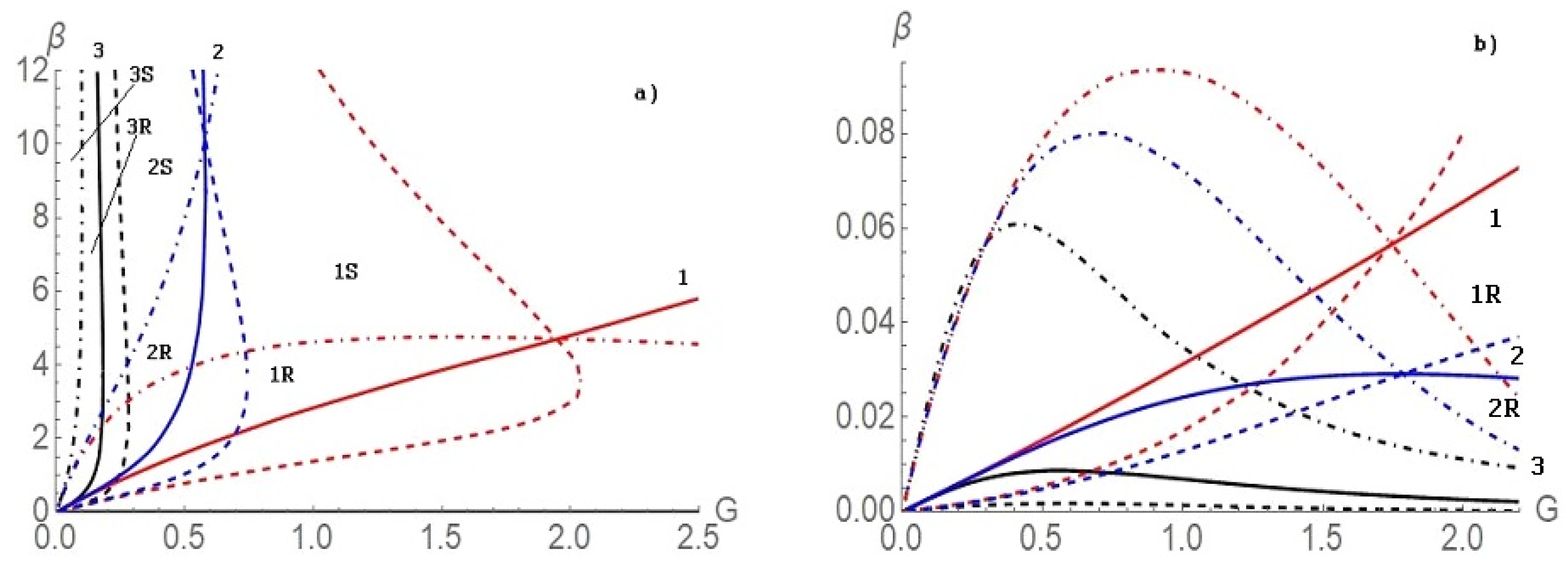
We consider the influence of the concentration of the surfactant on the pattern selection at very low values of the elasticity number. As shown in
Figure 2, even low concentration of the surfactant remarkably changes the pattern selection of the structures on the square lattice in the Fourier space. There are two regions of stationary pattern stability, one shown in
Figure 2a and another one, for small values of
, in
Figure 2b. Here the set #1 (red colored) belongs to the case without surfactant. The set #2 (blue colored) represents the case with
and the set #3 (black colored) corresponds to the case
. The marks on the Figure show the supercritical stability regions, and they include the number corresponding to the set number and the letter, “R” for stable rolls and “S” for stable squares. Here the solid lines are boundaries between supercritical and subcritical bifurcations for rolls (
). The dashed lines are similar boundaries for squares (
), and the dot-dashed lines, which correspond to the relation
, separate the regions of the stable rolls and stable squares.
Figure 2b shows domains at small
. Here the rolls are mainly selected, for greater values of
the squares are selected. Even a low concentration of the surfactant diminishes the stability domains. This effect is enhanced with the growth of the elasticity number.
Therefore, it was found that the most typical form of patterns is the roll pattern. Note that in a rectangular container with one size much longer than another one or in a narrow annular container of large radius, that pattern is the only possible kind of patterns.
In the next section, we investigate the instability of roll patterns with respect to one-dimensional disturbances breaking the spatial periodicity of patterns (Eckhaus instability).
4. Modulation of Roll Patterns
4.1. Amplitude Equations
We consider the roll patterns near the instability threshold,
In that region, the motionless state is unstable with respect to disturbances in the interval of wavenumbers of the width around , and their growth rate is .
Following the approach of Newell, Whitehead, and Segel [
11,
12], we introduce two spatial scales: (i) the scale
corresponding to the basic wavelength of patterns, and (ii) the scale
corresponding to the spatial modulation of patterns due to the superposition of Fourier components within and around the instability region. Also, we rescale the time variable:
The differential operators are transformed in the following way
Therefore, the solution at the leading order is
(
and
are the same as in the previous section). At the second order the solution is
The equation for the heat transfer, (2), at the second order gives us the relation between
and
:
At the third order the solvability condition yields the evolution equation for the amplitude
similar to that obtained by Golovin et al. [
13] in the problem of the interaction of the short-wave and long-wave instability modes:
The coefficients
are cumbersome and are not presented here. The equation for the surface deformation
which can be obtained from the kinematic Equation (1), as well as the equation for perturbations of surfactant concentration
, are obtained at the fourth order as (here we eliminated
using (31)):
where
The obtained system of Equations (31)–(33) describes the evolution of modulated rolls near the instability threshold. Recall that is the amplitude of the rolls (see (26)), while and are long-wave deformation of the free surface and concentration of the surfactant, respectively (see (27),(29)). Therefore, additional terms and reflect the influence of large-scale surface deformation and inhomogeneity of surfactant concentration on the roll-like Marangoni convection. In Equations (32) and (33) the term is due to a large-scale flow and a surfactant flux generated by the spatial inhomogeneity of the convection roll amplitude.
System (32)–(33) is solved under global conditions on
and
:
Here
is averaging over
; the appearance of convection cannot change the total volume of the liquid and the amount of the surfactant.
4.2. Equation for the Growth Rate
Now we consider the linear stability analysis of the spatially periodic roll patterns, in the framework of the system of Equations (31)–(34).
Let us consider the family of stationary roll patterns
The parameter
is the rescaled deviation of the wave number from the critical value
;
. Solutions (36), (26) describe the stationary spatially periodic supercritical convection with constant amplitude, without interfacial deformation and disturbance of the surfactant concentration independent of
.
To describe the roll stability, we add small perturbations to the roll amplitude and phase in the form where and are real functions of and .
Linearizing Equations (32)–(34), we obtain the following evolution equations for
and
Though the disturbances are real, one can perform the stability analysis using normal modes in the form
where the eigenvector
and the eigenvalue
can be complex.
Substituting these modes into (37)–(40) we obtain the following equation for the growth rate of the side-band instability:
where
and
It is known, see [
11], that the limit
is crucial for the long-wave modulations of the patterns. Assuming
, we obtain at the leading order,
We find that one root,
corresponding to amplitude modulation of the roll pattern, is negative, while other three roots tend to zero when
. For those roots, we obtain at the leading order
This equation describes the interaction of three “soft” (Goldstone) modes corresponding to definite symmetries of the problem, phase disturbances (translational invariance of the envelope function), surface deformation (conservation of the volume) and surfactant concentration disturbances (conservation of the amount of surfactant).
4.3. Stability in the Absence of Surfactant
First, let us consider the roll modulation in the absence of surfactant
. In that case, coefficients
and
in (32), (33) are equal to zero, hence those equations do not contain
. Equations (37)–(39) form a closed system, while Equation (40), which has no physical meaning, has the obvious solution
hence
Therefore, the dispersion relation (42) can be presented as
The analysis of the dispersion relation is reduced to the consideration of a quadratic equation,
where
and
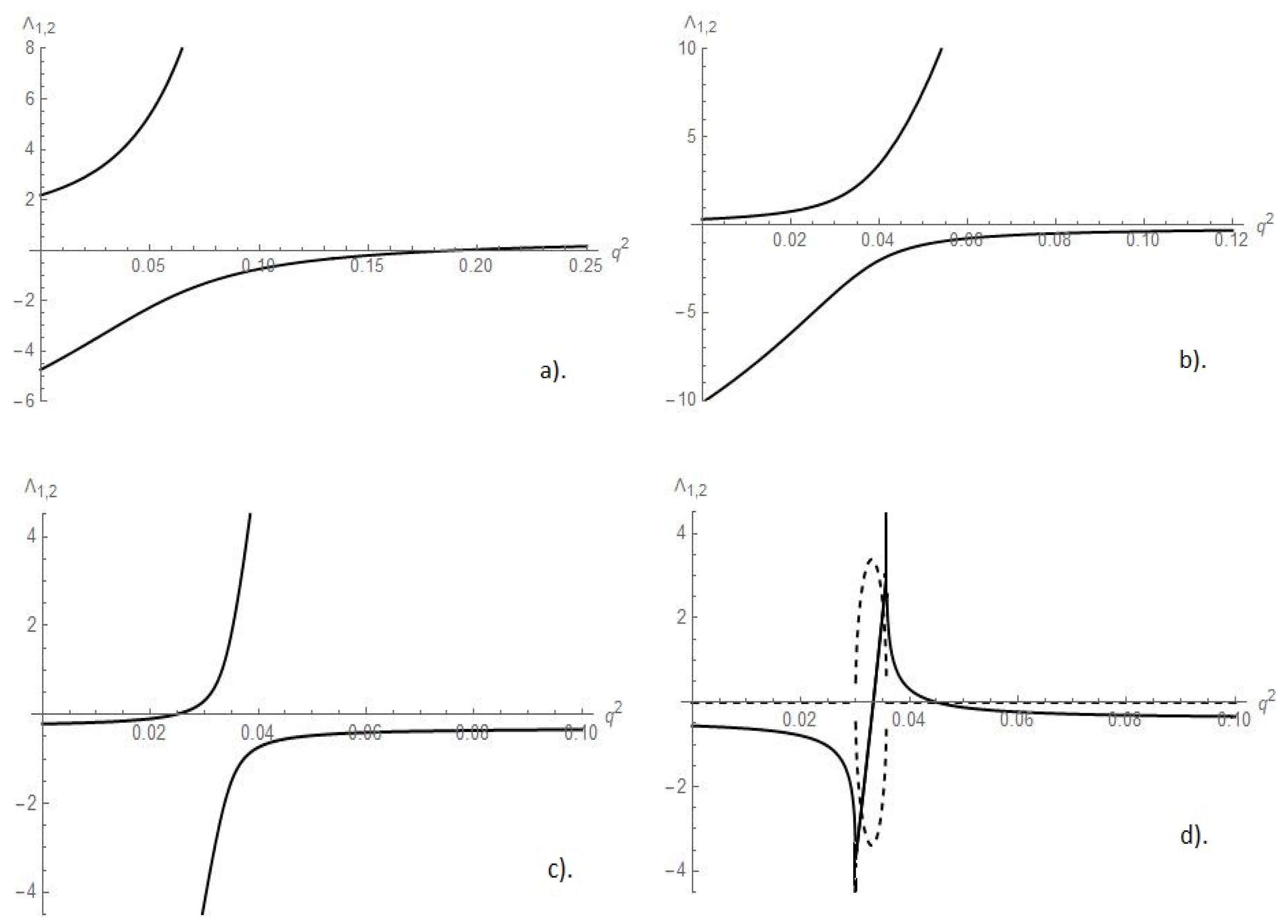
Equation (43) for the growth rate has two roots. Let us plot the growth rates as functions of for several values of at fixed parameter (parameters ).
Figure 3a shows the growth rate at
For
one root is positive and another one negative; for
, both roots are positive. We find that in this case the rolls with arbitrary values of
are monotonically unstable.
Figure 3b presents case of
where one growth rate is negative for all
, but the second one is positive in whole interval
0.112, where the roll solution (37) exists. Again, all the rolls are monotonically unstable. At
(
Figure 3c), in the range
the rolls are stable (both
are negative); for
between
and
one of the growth rates is positive, therefore we have unstable rolls. Starting from
the instability is oscillatory on the boundary of the stability interval of rolls. At
Figure 3d the dashed line describes the imaginary part of the growth rate. The rolls are stable when
and unstable (oscillatory or monotonically) when
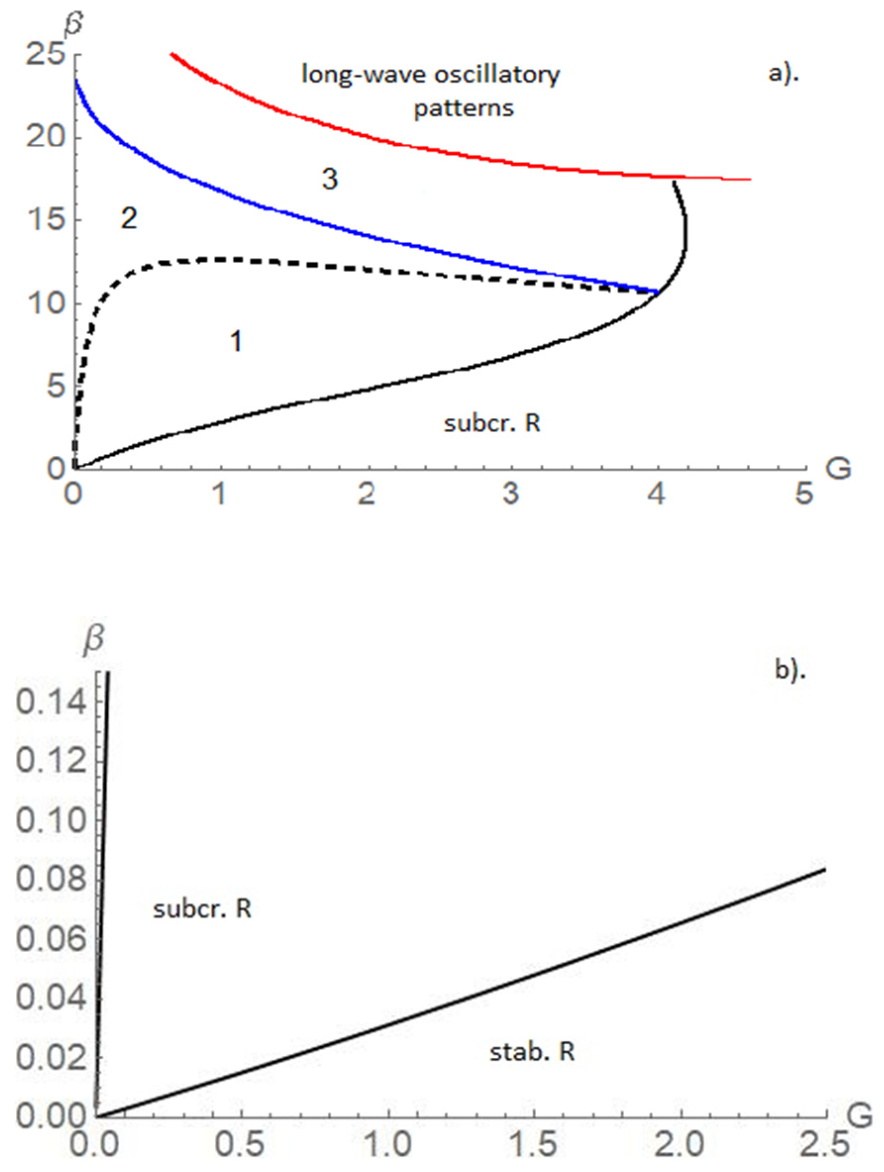
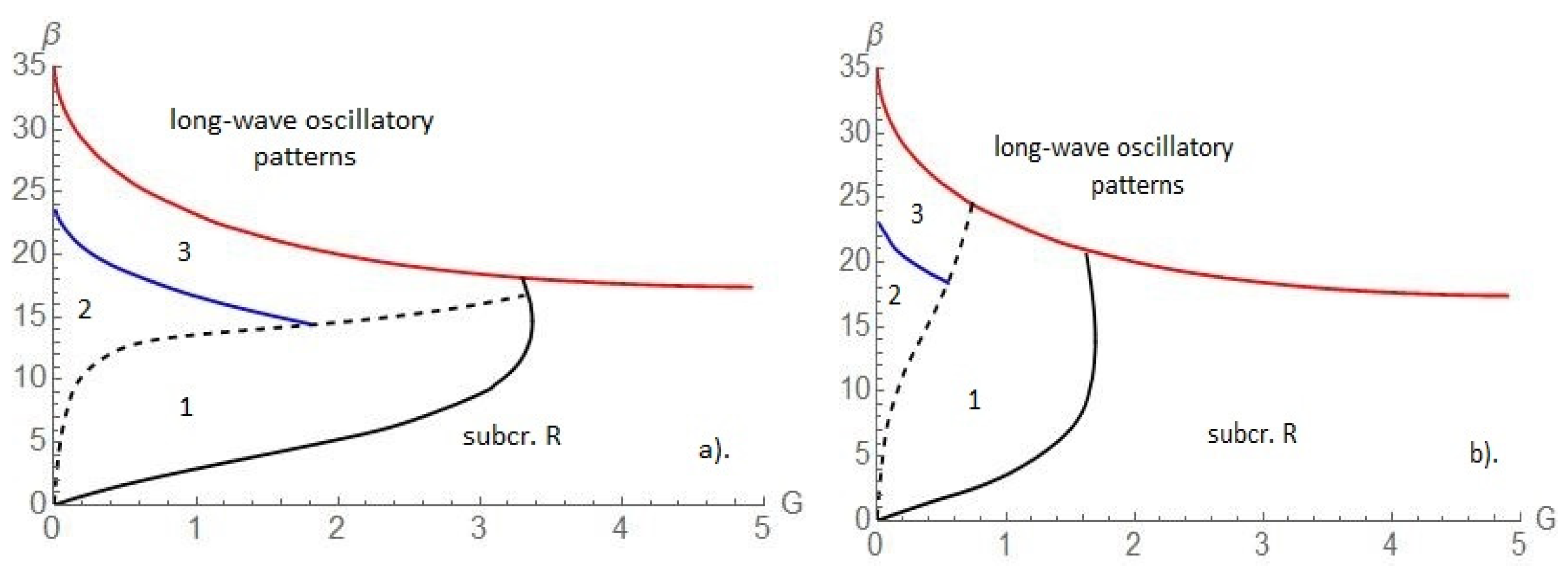
The stability map of the stationary rolls with respect to long-wave modulation is shown in
Figure 4. The black solid line here indicates the boundary between supercritical and subcritical regions for the rolls. We consider only the region of supercritical rolls (case
). The previous investigation of Shklyaev et al. [
5] shows the existence of long-wave oscillatory instability of the conductive state above the red solid line on
Figure 4. Therefore, the analysis of the modulational instability of rolls has to be done only between the black solid line and the red solid line, where there are three regions:
- (i)
region 1, where all the rolls are unstable with respect to modulations;
- (ii)
region 2, where the rolls are stable within the interval and monotonically unstable for ;
- (iii)
region 3, where the rolls are stable within the interval oscillatory unstable for slightly above , and oscillatory or monotonically unstable for any
All regions are shown in
Figure 4a. The values of
and
can be found analytically.
The boundary of the monotonic Eckhaus instability (
) is given by the relation
, hence
The quantity
is determined by the relation
hence
Figure 4b shows an additional region of stable rolls in the neighborhood of the origin (small values of
and
).
4.4. Influence of Insoluble Surfactant
As shown in our previous research [
10], even rather small quantity of insoluble surfactant on the free surface of liquid can significantly change the instability thresholds and creates new oscillatory regimes. That instability is determined by both the surface property of the surfactant (
) and its concentration (
) through the elasticity number
that includes both factors.
In the present paper, we consider the influence of a very small amount of insoluble surfactant on the modulation stability of stationary rolls. For this goal we use dispersion relation (42). From this relation the monotonic Eckhaus instability is determined by the relation
or
where
is the width of the existence interval of the periodic solutions (
), and
If the interaction of the roll convection with the deformations and disturbances of the surfactant concentration is switched off, i.e.,
or
, then
, and the classical result
is recovered. The expression for the oscillatory Eckhaus instability boundary
is cumbersome, and it is not presented here.
For plotting stability maps we take two values of the elasticity parameter:
and
In both cases the Lewis number was fixed at
The stability maps are shown in
Figure 5. Here
Figure 5a corresponds to the case
and
Figure 5b to
.
Comparing the stability maps with surfactant and without surfactant we conclude that the region of stable rolls shrinks with addition of the insoluble surfactant while the subcriticality region expands. The behavior of the growth rates in each of these regions (“1”, “2”, and “3”) are similar to those describing in the case without surfactant. The shrinking of the region of stable supercritical rolls means that with addition of an insoluble surfactant the appearance of a subcritical instability becomes more typical. Therefore, the linear stability analysis become inefficient, and the nonlinear analysis is unavoidable.
5. Conclusions
In the present paper we have studied a stationary Marangoni convection without and with insoluble surfactant spread over a deformable free surface. The analysis of nonlinear dynamics of perturbations near the instability threshold shows the existence of two kinds of steady supercritical periodic structures–rolls and squares. We investigated the dependence of their stability regions on the heat transfer at the liquid surface, characterized by Biot number, deformability of the free surface of the liquid characterized by Galileo number, and the action of the surfactant on the surface tension characterized by the elasticity number. The presented theory can be applied to different active agents on different surfaces, independently of the physico-chemical mechanism of the surface-tension decrease, on the condition of low solubility of the surfactant (the influence of the surfactant on the properties of the bulk liquid is assumed to be negligible).
It is shown how the regions of pattern selection change under the influence of the surfactant.
In addition, we carried out the linear analysis of modulational instability of stationary rolls near the bifurcation point. Using the weakly nonlinear analysis, the set of amplitude equations that describe large-scale one-dimensional (longitudinal) distortions of periodic roll patterns is derived. The stability maps of the stationary rolls with and without surfactant have been presented. The results indicate the existence of three regions of the supercritical rolls: (i) region where the rolls are unstable with respect to modulations; (ii) region where the rolls are stable within the interval and monotonically unstable for ; (iii) region where the rolls are stable within the interval oscillatory unstable for slightly above , and oscillatory or monotonically unstable for any
To check the results of described theory we propose performing an experiment on Marangoni convection in a rectangular container with one size much longer than another one or in a narrow annular container of large radius.

