Article

Bound Coherent Structures Propagating on the Free Surface of Deep Water

by
Dmitry Kachulin
1,2,*,
Sergey Dremov
1,2,* and
Alexander Dyachenko
3
1
Novosibirsk State University, 630090 Novosibirsk, Russia
2
Skolkovo Institute of Science and Technology, 121205 Moscow, Russia
3
Landau Institute for Theoretical Physics RAS, 142432 Chernogolovka, Russia
*
Authors to whom correspondence should be addressed.
Fluids 2021, 6(3), 115; https://doi.org/10.3390/fluids6030115
Submission received: 17 February 2021 / Revised: 5 March 2021 / Accepted: 9 March 2021 / Published: 12 March 2021
(This article belongs to the Special Issue Recent Advances in Free Surface Hydrodynamics)

Abstract

:
This article presents a study of bound periodically oscillating coherent structures arising on the free surface of deep water. Such structures resemble the well known bi-soliton solution of the nonlinear Schrödinger equation. The research was carried out in the super-compact Dyachenko-Zakharov equation model for unidirectional deep water waves and the full system of nonlinear equations for potential flows of an ideal incompressible fluid written in conformal variables. The special numerical algorithm that includes a damping procedure of radiation and velocity adjusting was used for obtaining such bound structures. The results showed that in both nonlinear models for deep water waves after the damping is turned off, a periodically oscillating bound structure remains on the fluid surface and propagates stably over hundreds of thousands of characteristic wave periods without losing energy.

1. Introduction

Nonlinear coherent structures arising on the free surface of fluid are of significant interest to oceanology. Today, there is a large number of theoretical models for describing such structures. In the case of shallow water it is the most famous Korteweg—De Vries (KdV) equation [1] and its various modifications and generalizations [2,3,4]. An undoubted advantage of studying such nonlinear objects in shallow water (in this case solitons or breathers) is the presence of a large number of models integrable in terms of the inverse scattering problem [5,6] and availability of exact analytical solutions.
In the case of deep water waves the only integrable model is the well-known Nonlinear Schrödinger equation (NLSE) [7]. The NLSE also has various exact solutions [8,9,10,11] and generalizations [12]. However, in practice, using these models may not be sufficient to describe the dynamics of deep water waves and various nonlinear wave phenomena since these models are derived in the assumption of spectral width narrowness which significantly limits their range of applicability. In this case, it is necessary to use more accurate models such as the super-compact Dyachenko-Zakharov equation (SCDZE) [13] or the full system of nonlinear equations for an ideal potential fluid written in conformal variables [14,15]. In [16], the authors showed that the full model also has a solution in the form of a giant breather. The classical NLSE soliton was used as the initial condition for obtaining such a solution. This discovery was the starting point for further experimental observation and research of such breathers on the surface of deep water [17,18,19,20]. It was shown in [21] that breather solution can be found numerically by using the Petviashvili method [22] in the model of SCDZE.
The SCDZE can be rewritten in terms of an envelope wave packet [23]. Under the assumption that the spectral width is narrow it can be reduced to the NLSE, and the SCDZE breather would then correspond to the NLSE envelope soliton. However, despite some similarities, the behaviour of breathers and solitons can differ significantly. For example, it was shown in work [24] that there are significant differences in the interaction of a pair of breathers and a pair of solitons. In the SCDZE there is an energy exchange between breathers depending on their relative phase. Moreover, they change their amplitudes and velocities during the interaction, which is not observed for solitons in the fully integrable model of NLSE.
It should be noted that, so far, in the SCDZE, only stable solutions in the form of a single breather are known. However, an unexpected result was obtained in [25], where multiple collisions of breathers in the periodic domain were studied. It was shown that the only one coherent structure remained at the end regardless of the breathers number and initial parameters. Still, the scenarios of long-time dynamics of the system could be different. In some cases, breathers were coupled into a single periodically oscillating structure resembling the well known NLSE bi-soliton solution [8,26]. This coupled solution allowed us to assume that the more accurate models also have solutions similar to the NLSE bi-solitons, and these solutions can be found numerically or even analytically. This work is devoted to the search for such solutions, as well as to the study of their characteristics.

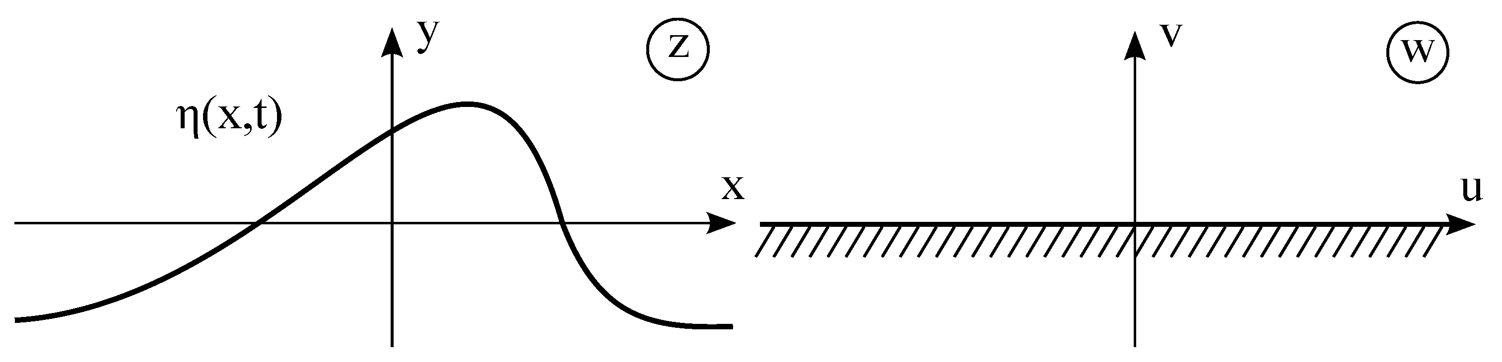
2. Deep Water Wave Equations

The fully nonlinear 2D equations describing gravity waves on the surface of ideal deep fluid are well known and can be written as:
ϕ x x + ϕ y y = 0 ( ϕ y 0 , y ) , η t + η x ϕ x = ϕ y y = η , ϕ t + 1 2 ( ϕ x 2 + ϕ y 2 ) + g η = 0 y = η .
Here x and y are the horizontal and vertical coordinates, t is time, g is the free-fall acceleration, η ( x , t ) is the shape of the surface, ϕ ( x , y , t ) is the hydrodynamic potential inside the fluid.
One-dimensional potential flow of an ideal fluid of infinite depth in the presence of gravity is a Hamiltonian system. As was shown by Zakharov [27], the surface elevation η ( x , t ) and the velocity potential at the surface ψ ( x , t ) = ϕ ( x , y , t ) | y = η of the fluid are canonically conjugated variables and satisfy the following Hamilton’s equations:
ψ t = δ H δ η , η t = δ H δ ψ .
Here H is the Hamiltonian, that is, total energy of the fluid:
H = 1 2 d x η | ϕ | 2 d y + g 2 η 2 d x .
In order to obtain and further investigate the bound coherent structures, we will use two models for deep water waves in our work—the super-compact Dyachenko-Zakharov equation (SCDZE) obtained from truncated Hamiltonian when considering waves propagating in the same direction (Section 3) and the full system of nonlinear equations for an ideal potential incompressible fluid written in conformal variables (Section 4).

3. Bound Structures in the Super Compact Dyachenko-Zakharov Equation

Assuming that wave steepness is small, the Hamiltonian can be represented as an infinite power series of η and ψ (see [27]). We consider this series up to the fourth order term:
H = 1 2 ( g η 2 + ψ k ^ ψ ) d x 1 2 { ( k ^ ψ ) 2 ( ψ x ) 2 } η d x + 1 2 { ψ x x η 2 k ^ ψ + ψ k ^ ( η k ^ ( η k ^ ψ ) ) } d x .
Here, operator k ^ means multiplication by | k | in k-space.
Equations of motion (2) with truncated Hamiltonian (4) can be used for numerical simulations of water surface dynamics [28]. However, they are not convenient for analytic study because η ( x , t ) and ψ ( x , t ) are not optimal canonical variables. Since the considered system is Hamiltonian, one can choose better Hamiltonian variables by performing a proper canonical transformation. In 2017, the most optimal canonical transformation from the pair of classical physical Hamiltonian variables η ( x , t ) and ψ ( x , t ) to normal complex variable c ( x , t ) was found. It not only cancels non-resonant third and fourth-order terms, but greatly simplifies the expression for the Hamiltonian when considering unidirectional waves (see [13]). This canonical transformation can be written as power series of c k up to the third order:
η k = η k ( 1 ) + η k ( 2 ) + η k ( 3 ) ψ k = ψ k ( 1 ) + ψ k ( 2 ) + ψ k ( 3 )
and is described in detail in [13]. As a result of the transformation the Hamiltonian takes the following form in x-space:
H = c * V ^ k c d x + 1 2 i 4 ( c 2 x c * 2 c * 2 x c 2 ) | c | 2 k ^ ( | c | 2 ) d x .
Here, operator V ^ k is multiplication by ω k k in Fourier space. Then, the equation of motion or the super compact Dyachenko-Zakharov equation (SCDZE) for unidirectional deep water waves has the following form:
c t + i ω ^ k c i x + | c | 2 c x = x + k ^ | c | 2 c .
Here, operator ω ^ k is a Fourier multiplier by the g k , where g is free fall acceleration. Operator x + corresponds to i k θ ( k ) in Fourier space, where θ ( k ) is Heaviside step function.
Physical variables of surface η ( x , t ) and potential ψ ( x , t ) can be recovered by canonical transformation (see details in [13]) the first and the second order terms of which can be written in x –space in a compact way:
η ( 1 ) ( x ) = 1 2 g 1 4 ( k ^ 1 4 c ( x ) + k ^ 1 4 c ( x ) * ) , ψ ( 1 ) ( x ) = i g 1 4 2 ( k ^ 3 4 c ( x ) k ^ 3 4 c ( x ) * ) , η ( 2 ) ( x ) = k ^ 4 g [ k ^ 1 4 c ( x ) k ^ 1 4 c * ( x ) ] 2 , ψ ( 2 ) ( x ) = i 2 [ k ^ 1 4 c * ( x ) k ^ 1 4 c * ( x ) k ^ 1 4 c ( x ) k ^ 1 4 c ( x ) ] + 1 2 H ^ [ k ^ 1 4 c ( x ) k ^ 1 4 c * ( x ) + k ^ 1 4 c * ( x ) k ^ 1 4 c ( x ) ] .
Here, H ^ is Hilbert transformation with eigenvalue i sign ( k ) and operators k ^ α act in Fourier space as multiplication by | k | α .
The SCDZE has a breather solution in the following form:
c ( x , t ) = c b r x ω k 0 2 k 0 t ; k 0 , δ e i k 0 x i ω k 0 t i δ t .
Breather solution (9) is determined by two parameters: k 0 is a carrier wave number, and δ . It can be found numerically only by the Petviashvili method (see details in [13]). It was found in [21] that the SCDZE is not integrable so that the collision of a pair of breathers is not purely elastic and is accompanied by an exchange of energy between breathers and the radiation of incoherent waves (see earlier papers [21,29], and also [20,24]).
It was observed for the first time in [25] that a collision of two single breathers with very close velocities could result in the formation of a periodically oscillating structure resembling the NLSE bi-soliton. Therefore, the obvious step to obtain the bound structure is to take two single breathers and then set them at the same point in space as initial conditions.

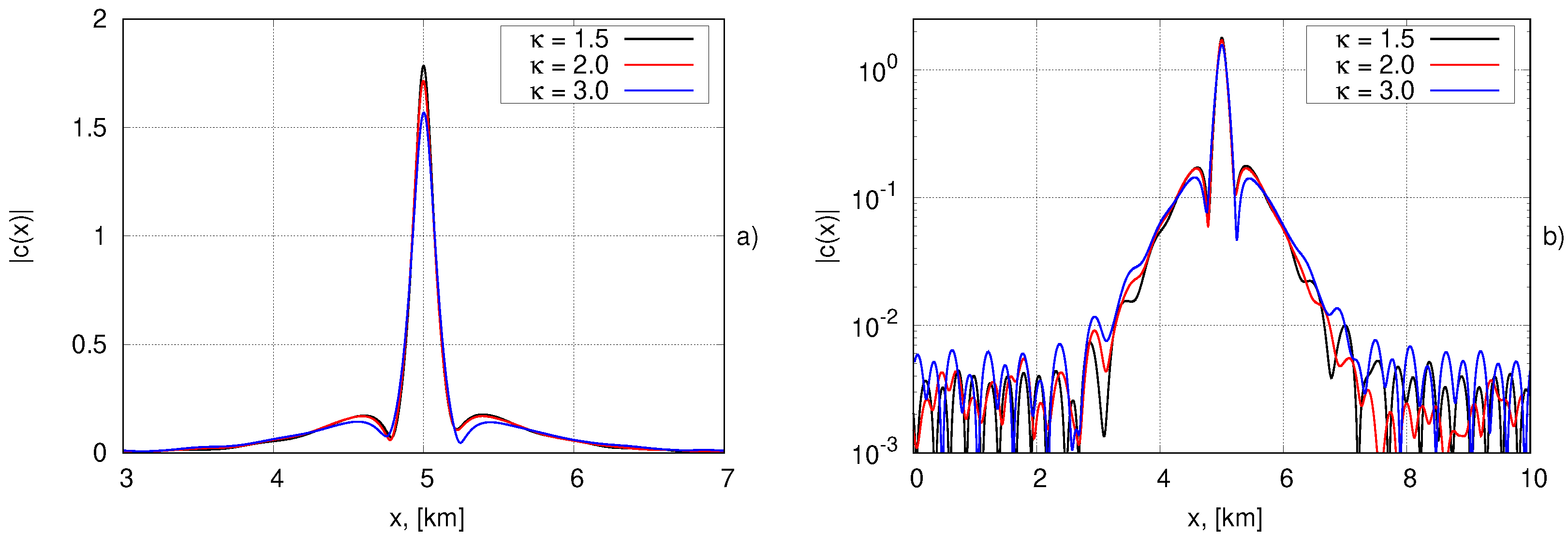
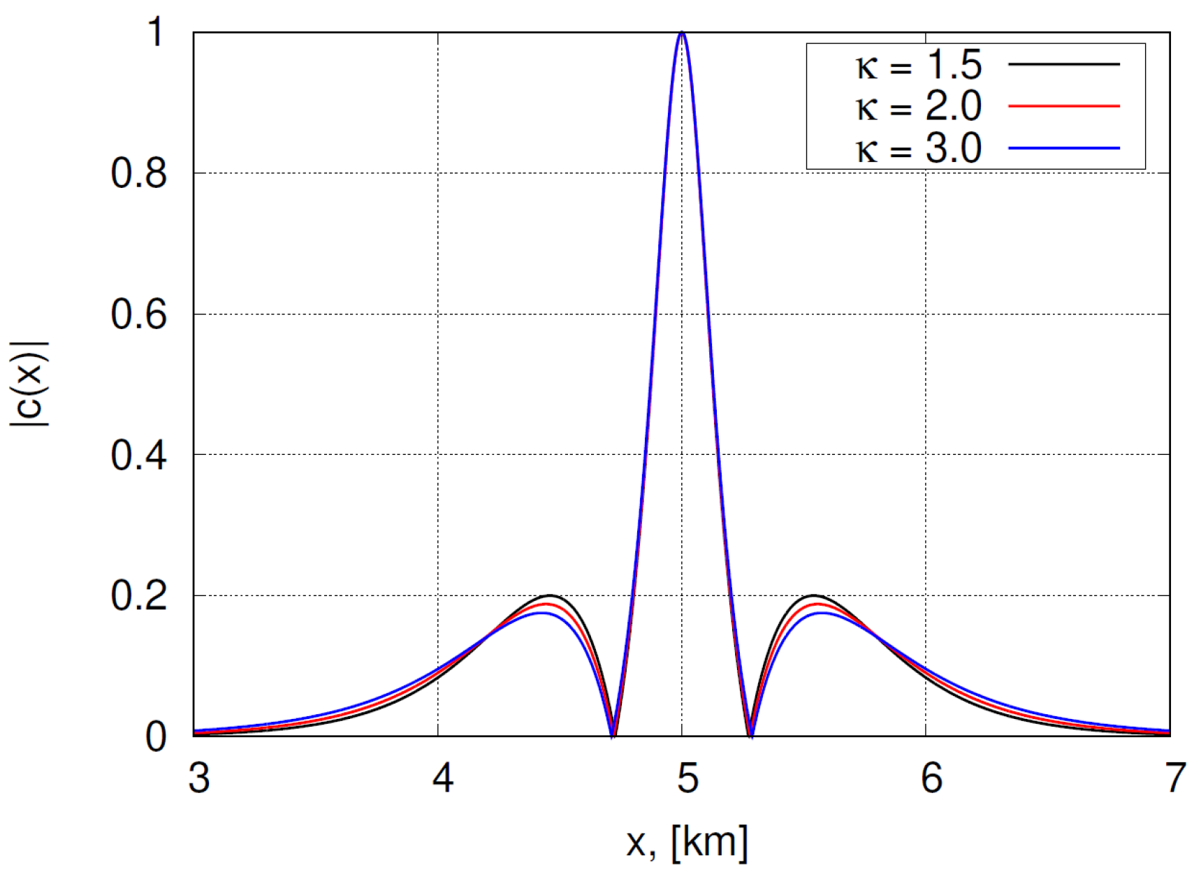
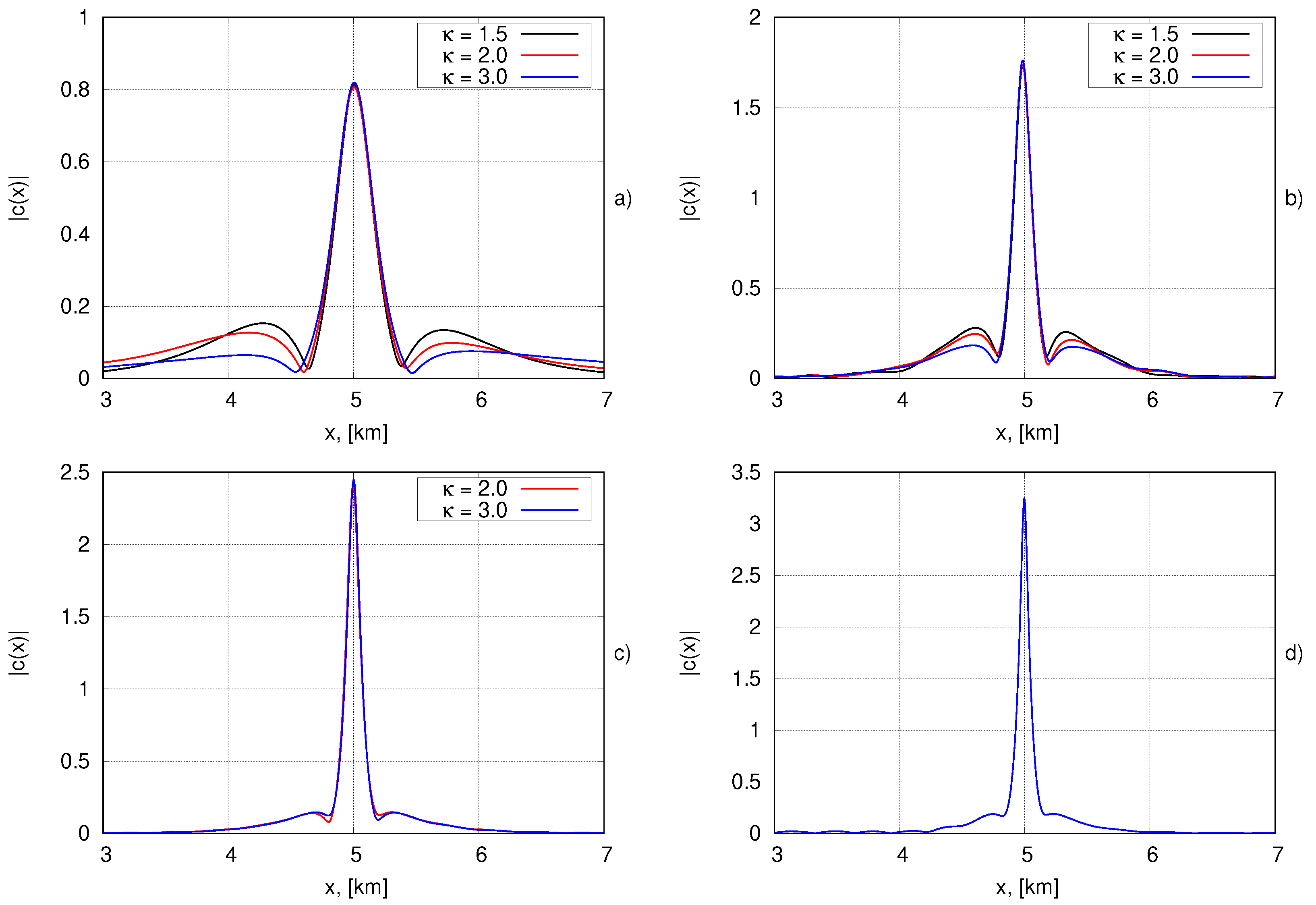
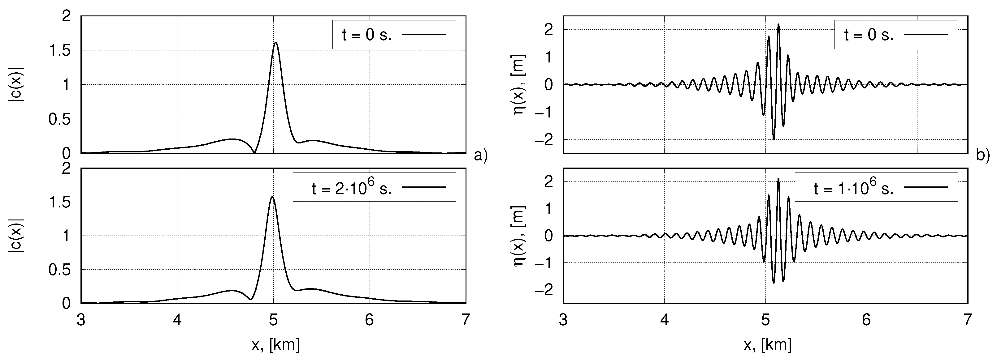
3.1. Numerical Method for Obtaining Bound Structures. Experiments with Two Breathers

Numerical simulations were carried out in the periodic domain with length L. The SCDZE was solved using the pseudo-spectral Fourier method, and the fourth-order Runga-Kutta method was applied to calculate time evolution. The FFTW3 library [30] was used for the fast Fourier transform procedure. The multiplication of grid functions was carried out in x-space; the direct and inverse Fourier transform were used for calculating derivatives and non-local terms.
The algorithm used for finding a solution is very similar to the one described in [16]. The main defining parameters were wave steepness μ and amplitude ratio κ = C 1 C 2 , where C 1 and C 2 —amplitude of the corresponding breather. In the process of calculating the time evolution the initial structure begins to radiate incoherent waves. Consequently, the steepness of the resulting structure will always be less than the steepness of the initial one. Thus, it is necessary to distinguish between initial steepness and resulting steepness. We will denote them as μ i n i and μ f i n respectively. Here we also note that we define amplitude ratio κ only at the initial moment of time. The damping procedure was used to remove radiation and for this, a term of the following form was added to the right-hand side of SCDZE:
c ( x , t ) t = γ f ( x ) c ( x , t )
f ( x ) = c o s 6 ( π x L ) .
Selected function f ( x ) and coefficient γ concentrate the damping at the edges of the domain without affecting the structure itself, which is always in the center of the domain. To keep the solution in the center, the velocity of the reference frame was constantly adjusted. Coefficient γ should not be chosen too high to prevent numerical instability. On the other hand, it should also not be too small; otherwise, the resulting radiation will not be damped. We chose γ in the range of 10 2 10 3 in our experiments.
As mentioned earlier, we first set the initial conditions in the form of two single breathers found by the Petviashvili method and placed them at one point of the domain. As one can see from Figure 1, an oscillating structure is formed with time and stably exists for 10 6 seconds for any amplitude ratio κ . Initial steepness μ i n i was 0.2 while resulting steepness μ f i n reaches ≈0.18. We plot these profiles after the damping process is switched off, the moment in time t itself does not matter in principle since these structures are periodic in time. The profiles are plotted in approximately the same phase to be compared with each other. The damping process itself lasted 3 × 10 5 seconds, damping coefficient γ was equal to 10 3 . The radiation level does not exceed 0.01 or 0.5% of maximum amplitude. The value of amplitude ratio κ does not significantly affect the resulting structure. A further increase in the breathers amplitudes results in a significant amplitude amplification during their interaction and wave breaking.
The full long film with the procedure of damping and further dynamics of the bound structure with μ i n i = 0.2 , κ = 1.5 and μ f i n 0.18 up to the 10 6 seconds can be found at the following link (accessed on 11 March 2021): http://kachulin.itp.ac.ru/mdpi-2021-films/SCEq-2br-mu018-l.mp4.
The short film with more detailed dynamics of the structure during the oscillation period can be found here (accessed on 11 March 2021): http://kachulin.itp.ac.ru/mdpi-2021-films/SCEq-2br-mu018-s.mp4.

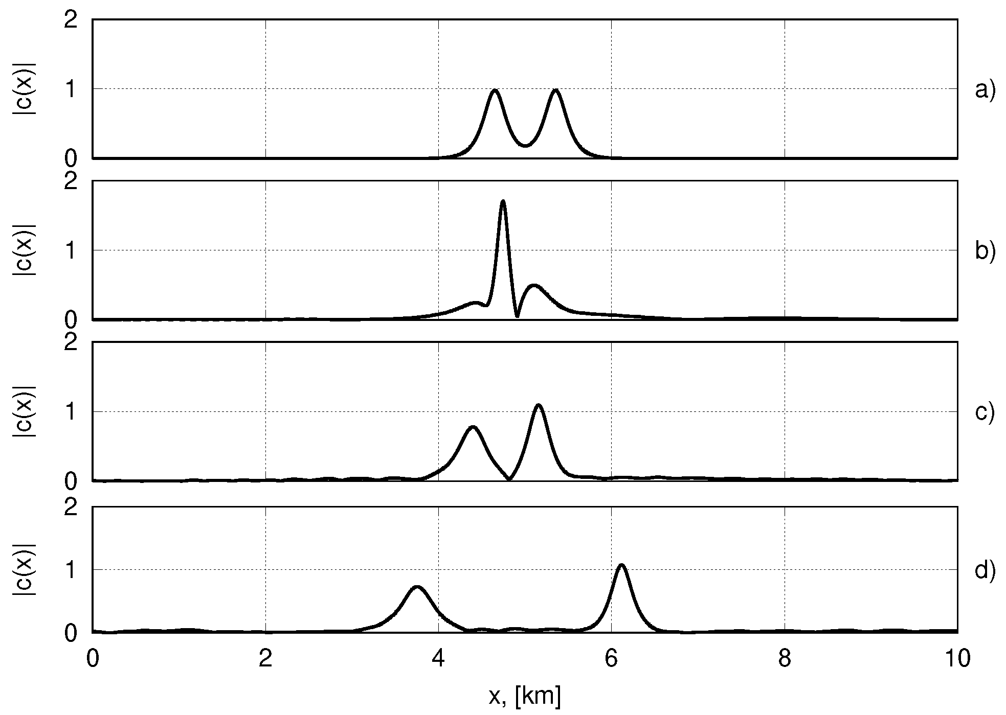
3.2. Numerical Method for Obtaining Bound Structures. Experiments with Bi-Solitons of the NLSE

Equation (7) can be re-written in terms of envelope of wave packet C ( x , t ) . If we suppose that the Fourier spectrum of waves has a maximum at k = k 0 we can introduce envelope function C ( x , t ) :
c ( x , t ) = C ( x , t ) e i ( k 0 x ω k 0 t ) ,
where ω k 0 = g k 0 is the corresponding linear frequency. Using Equation (10), which is actually canonical transformation, one can easily derive the exact equation for the envelope C that we named the “Dyachenko–Zakharov envelope equation” [23]. This equation written in the reference frame moving with the group velocity V 0 = ω k 0 2 k 0 has the following form:
C t + i ω k 0 + k ω k 0 ω k 0 k 0 k ^ θ ^ k 0 + k C + i k 0 2 θ ^ k 0 + k | C | 2 C + k 0 θ ^ k 0 + k C x | C | 2 + 2 | C | 2 C x i k ^ ( | C | 2 ) C θ ^ k 0 + k x k ^ ( | C | 2 ) C + i | C | 2 C x = 0 .
The equation was derived without any assumptions about the spectral width of the wave packet. Moreover, Equation (11) is the exact envelope form of Equation (7) and has the same range of applicability. One can extract the nonlinear Schrödinger (NLS) equation in the assumption of narrowband spectrum:
C t + i ω k 0 8 k 0 2 2 C x 2 + i k 0 2 | C | 2 C = 0 .
The NLSE bi-soliton solutions ([8,26]) are well-known examples of bound nonlinear coherent structures. Thus, based on the above approximation, another way to set the initial wave field is to use the NLSE bi-solitons the explicit expression for which has the following form:
C b s ( x , t ) = 2 C 1 C 2 C 1 + C 2 C 1 cosh 2 C 2 k 0 2 ω k 0 ( x x 2 ) e 1 2 i k 0 2 C 1 2 t C 2 cosh 2 C 1 k 0 2 ω k 0 ( x x 1 ) e 1 2 i k 0 2 C 2 2 t C 1 C 2 C 1 + C 2 2 cosh 2 k 0 2 ω k 0 C 1 ( x x 1 ) + C 2 ( x x 2 ) + cosh 2 k 0 2 ω k 0 C 1 ( x x 1 ) C 2 ( x x 2 ) 4 C 1 C 2 ( C 1 + C 2 ) 2 cos C 1 2 C 2 2 k 0 2 2 t .
The solution is periodic in time with T = 4 π k 0 2 ( C 1 2 + C 2 2 ) , C 1 and C 2 — solitons amplitude. We introduce also the variable κ = C 1 C 2 which plays a role in the dynamics of the resulting structure. This parameter is also defined only at the initial moment of time.
The examples of used as initial conditions bi-solitons with μ i n i = 0.1 and different κ values are shown in Figure 2. The plotted profiles correspond to Equation (13) at t = 0 , and one can see that there are two simultaneous zeros of | c ( x ) | at such a phase. The calculation process is not much different—the bi-soliton begins to radiate, it is suppressed by damping procedure and then it turns off. Figure 3 shows | c ( x ) | for the bound structures resulted from the initial NLSE bi-solitons with different amplitude ratios κ and initial steepness μ i n i = 0.1 (a), 0.2 (b), 0.3 (c) and 0.4 (d). As can be seen, structures exist in a wide range of defining parameters μ and κ . The bound objects stably propagate for at least hundreds of thousands of wave periods T = 2 π w 0 10 s . The damping coefficient γ was 10 3 . The duration of damping was chosen in such a way as to control the radiation level in the range of 10 2 10 3 . As μ i n i increases, the influence of κ becomes insignificant. In particular, in the case of μ i n i = 0.4, the variable of κ does not affect the profile of the resulting structure at all. Another feature is that increasing μ i n i and κ results in a greater deviation from the original bi-soliton solution. Note that in all obtained structures two zeros of | c ( x ) | can occur only alternately, but not simultaneously, unlike the NLSE bi-soliton solution.
The full long film with damping procedure and further dynamics up to 10 6 seconds of the bound structure resulted from the NLSE bi-soliton with μ i n i = 0.3 , κ = 1.5 and μ f i n 0.25 can be found at the following link (accessed on 11 March 2021): http://kachulin.itp.ac.ru/mdpi-2021-films/SCEq-mu025-l.mp4. The small window at the top right shows the dynamics of the structure on a logarithmic scale to see the radiation level.
The short film with more detailed dynamics of the bound structure during the oscillation period can be found here (accessed on 11 March 2021): http://kachulin.itp.ac.ru/mdpi-2021-films/SCEq-mu025-s.mp4.
An interesting feature when using bi-soliton as an initial condition is that there is a range of parameters μ and κ at which obtaining a bound structure becomes impossible. Instead, there is a split of bi-soliton in two separate solitons (Figure 4). The phenomenon manifests itself at small amplitude ratios ( κ < 1.25 ) depending on the steepness, but at κ = 1.1 bi-soliton splits at any value of μ within the applicability of the SCDZE. In the case of initial conditions in the form of two single breathers, no separation occurs.
The film with NLSE bi-soliton splitting can be found here (accessed on 11 March 2021): http://kachulin.itp.ac.ru/mdpi-2021-films/Bi-Sol-split.mp4.

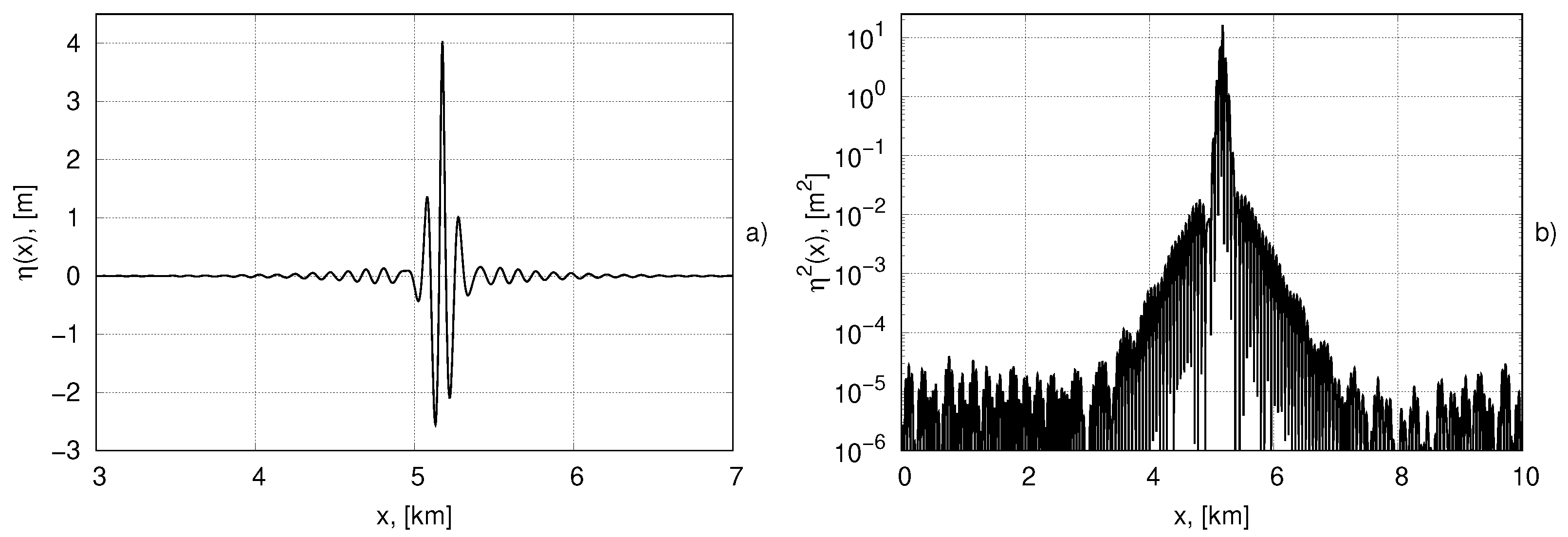
4. Bound Structures in the Full System of Nonlinear Equations

Following work [14] we perform conformal mapping of the free surface liquid domain z = x + i y confined by a free boundary y = η ( x , t ) onto a half-plane of new complex variable w = u + i v having a fixed boundary v 0 –– see Figure 5. This transformation can be written in the following form:
y = H ^ ( x ( u , t ) u ) , x ( u , t ) = u H ^ y ( u , t ) .
Then, we use the following variables suggested by Dyachenko [15]:
R = 1 z w , V = i Φ z = i Φ w z w .
We define functions U and B using the Hilbert operator and the projection operator P ^ = 1 2 ( 1 + i H ^ ) as:
U = P ^ ( V R * + V * R ) , B = P ^ ( V V * ) .
Here and below the asterisks stands for complex conjugation. In new variables (15) the fully nonlinear (RV) equations have the following form:
R t = i ( U R w R U w ) , V t = i ( U V w R B w ) + g ( R 1 ) ,
with the boundary conditions:
R 1 , V 0 , at v .
Figure 6 shows the structure obtained from the original bi-soliton with μ i n i = 0.2 and κ = 1.5 . The maximum steepness of the obtained structure μ f i n reaches ≈ 0.175. The structure propagated stably for 2 × 10 6 seconds without losing energy in the SCDZE model (a). After completing the calculation in the SCDZE we used canonical transformations (8) from variable c ( x ) to variables η and ψ . Further, variables R and V were obtained using (15), and we continued the simulating process in the model of RV equations (b). The structure also propagated stably for 1 × 10 6 seconds within this model.
The bound structure can also be obtained in the exact RV model by specifying two breathers or the NLSE bi-solitons as the initial conditions. Figure 7 shows the example of bound structure with μ f i n 0.25. It was obtained using the NLSE bi-soliton with μ i n i = 0.3 and κ = 1.5 as the initial condition. Panel (a) shows the surface profile η ( x ) while panel (b) shows a squared surface η 2 ( x ) in logarithmic scale to monitor the radiation level. As in other cases, the structure exists stably and does not lose energy. If initial steepness μ i n i exceeds 0.5, it will always result in the splitting of the bound state mentioned earlier regardless of the initial conditions and the choice of κ .
The full long film with the procedure of damping and further dynamics of this structure up to the 10 6 seconds in the model of RV equations can be found at the following link: http://kachulin.itp.ac.ru/mdpi-2021-films/RV-mu025-l.mp4.
The short film with detailed dynamics of bound structure during one period in the model of RV equations can be found here: http://kachulin.itp.ac.ru/mdpi-2021-films/RV-mu025-s.mp4.

5. Conclusions

We investigated bound coherent structures in the model of SCDZE for unidirectional deep water waves and the full system of nonlinear equations for potential flows of an ideal incompressible fluid written in conformal variables. Two single breathers placed at one point of the domain, as well as well-known NLSE bi-soliton solutions were used as initial conditions in numerical experiments. In the simulations the initial structure radiated incoherent waves that were suppressed by the damping mechanism. It was shown in both variants of initial conditions that after the damping procedure is turned off, the remaining bound structure propagates stably on the surface of the fluid and does not lose energy for hundreds of thousands of characteristic wave periods. Such structures were obtained in a wide range of determining parameters—steepness and amplitude ratios. It was also revealed that there is a range of parameters at which it is impossible to obtain the bound structure. Instead, there is a split of initial structure into two separate ones. The resulting bound structures may turn out to be new solutions to the equations used and we hope that further research will help understand their nature in more detail.

Author Contributions

Investigation, writing—review and editing, D.K., S.D., A.D.; software and visualisation, D.K., S.D.; writing—original draft preparation, D.K., S.D., A.D. All authors have read and agreed to the published version of the manuscript.

Funding

The Russian Science Foundation Grant No. 19-72-30028 and The Russian Foundation for Basic Research Grant No. 20-31-90093

Acknowledgments

The study reported in Section 4 was supported by the Russian Science Foundation (Grant No. 19-72-30028 to D.K., S.D.). The study reported in Section 3 was funded by RFBR according to the research project No. 20-31-90093 (D.K., S.D.). Simulations were performed at the Novosibirsk Supercomputer Center of Novosibirsk State University.

Conflicts of Interest

The authors declare no conflict of interest.

Abbreviations

The following abbreviations are used in this manuscript:
NLSEnonlinear Schrödinger equation
SCDZEsuper compact Dyachenko-Zakharov equation
RV (equations)fully nonlinear equations written in conformal variables

References

  1. Korteweg, D.J.; De Vries, G.X.L.I. On the change of form of long waves advancing in a rectangular canal, and on a new type of long stationary waves. Lond. Edinb. Dublin Philos. Mag. J. Sci. 1895, 39, 422–443. [Google Scholar] [CrossRef]
  2. Kadomtsev, B.B.; Petviashvili, V.I. On the stability of solitary waves in weakly dispersing media. Sov. Phys. Dokl. 1970, 15, 539–541. [Google Scholar]
  3. Boussinesq, J. Théorie des ondes et des remous qui se propagent le long d’un canal rectangulaire horizontal, en communiquant au liquide contenu dans ce canal des vitesses sensiblement pareilles de la surface au fond. J. Math. Pures Appl. 1872, 17, 55–108. [Google Scholar]
  4. Davey, A.; Stewartson, K. On three-dimensional packets of surface waves. Proc. R. Soc. London. Math. Phys. Sci. 1974, 338, 101–110. [Google Scholar]
  5. Gardner, C.S.; Greene, J.M.; Kruskal, M.D.; Miura, R.M. Method for solving the Korteweg-deVries equation. Phys. Rev. Lett. 1967, 19, 1095. [Google Scholar] [CrossRef]
  6. Zakharov, V.E.; Shabat, A.B. A scheme for integrating the nonlinear equations of mathematical physics by the method of the inverse scattering problem. I. Funct. Anal. Its Appl. 1974, 8, 226–235. [Google Scholar] [CrossRef]
  7. Zakharov, V.E.; Manakov, S. On the complete integrability of a nonlinear Schrödinger equation. Theor. Math. Phys. 1974, 19, 551–559. [Google Scholar] [CrossRef]
  8. Peregrine, D.H. Water waves, nonlinear Schrödinger equations and their solutions. ANZIAM J. 1983, 25, 16–43. [Google Scholar] [CrossRef] [Green Version]
  9. Akhmediev, N.; Eleonskii, V.; Kulagin, N. Generation of periodic trains of picosecond pulses in an optical fiber: Exact solutions. Sov. Phys. JETP 1985, 62, 894–899. [Google Scholar]
  10. Kuznetsov, E.A. Solitons in a parametrically unstable plasma. DoSSR 1977, 236, 575–577. [Google Scholar]
  11. Ma, Y.C. The perturbed plane-wave solutions of the cubic Schrödinger equation. Stud. Appl. Math. 1979, 60, 43–58. [Google Scholar] [CrossRef]
  12. Dysthe, K.B. Note on a modification to the nonlinear Schrödinger equation for application to deep water waves. Proc. R. Soc. London. Math. Phys. Sci. 1979, 369, 105–114. [Google Scholar]
  13. Dyachenko, A.; Kachulin, D.; Zakharov, V.E. Super compact equation for water waves. J. Fluid Mech. 2017, 828, 661–679. [Google Scholar] [CrossRef] [Green Version]
  14. Dyachenko, A.I.; Kuznetsov, E.A.; Spector, M.; Zakharov, V.E. Analytical description of the free surface dynamics of an ideal fluid (canonical formalism and conformal mapping). Phys. Lett. A 1996, 221, 73–79. [Google Scholar] [CrossRef]
  15. Dyachenko, A.I. On the Dynamics of an Ideal Fluid with a Free Surface. Dokl. Math. 2001, 63, 115–117. [Google Scholar]
  16. Dyachenko, A.I.; Zakharov, V.E. On the formation of freak waves on the surface of deep water. JETP Lett. 2008, 88, 307. [Google Scholar] [CrossRef]
  17. Slunyaev, A. Numerical simulation of “limiting” envelope solitons of gravity waves on deep water. J. Exp. Theor. Phys. 2009, 109, 676–686. [Google Scholar] [CrossRef]
  18. Slunyaev, A.; Clauss, G.F.; Klein, M.; Onorato, M. Simulations and experiments of short intense envelope solitons of surface water waves. Phys. Fluids 2013, 25, 067105. [Google Scholar] [CrossRef] [Green Version]
  19. Slunyaev, A.; Klein, M.; Clauss, G.F. Laboratory and numerical study of intense envelope solitons of water waves: Generation, reflection from a wall, and collisions. Phys. Fluids 2017, 29, 047103. [Google Scholar] [CrossRef] [Green Version]
  20. Kachulin, D.; Dyachenko, A.; Gelash, A. Interactions of coherent structures on the surface of deep water. Fluids 2019, 4, 83. [Google Scholar] [CrossRef] [Green Version]
  21. Dyachenko, A.I.; Kachulin, D.; Zakharov, V.E. On the nonintegrability of the free surface hydrodynamics. JETP Lett. 2013, 98, 43–47. [Google Scholar] [CrossRef]
  22. Petviashvili, V.I. Equation of an extraordinary soliton. FizPl 1976, 2, 469–472. [Google Scholar]
  23. Dyachenko, A.; Kachulin, D.; Zakharov, V.E. Envelope equation for water waves. J. Ocean. Eng. Mar. Energy 2017, 3, 409–415. [Google Scholar] [CrossRef]
  24. Kachulin, D.; Gelash, A. On the phase dependence of the soliton collisions in the Dyachenko–Zakharov envelope equation. Nonlinear Process. Geophys. 2018, 25, 553–563. [Google Scholar] [CrossRef] [Green Version]
  25. Kachulin, D.; Dyachenko, A.; Dremov, S. Multiple Soliton Interactions on the Surface of Deep Water. Fluids 2020, 5, 65. [Google Scholar] [CrossRef]
  26. Shabat, A.; Zakharov, V. Exact theory of two-dimensional self-focusing and one-dimensional self-modulation of waves in nonlinear media. Sov. Phys. JETP 1972, 34, 62. [Google Scholar]
  27. Zakharov, V.E. Stability of periodic waves of finite amplitude on the surface of a deep fluid. J. Appl. Mech. Tech. Phys. 1968, 9, 190–194. [Google Scholar] [CrossRef]
  28. Korotkevich, A.; Pushkarev, A.; Resio, D.; Zakharov, V.E. Numerical verification of the weak turbulent model for swell evolution. Eur. J. Mech. B/Fluids 2008, 27, 361–387. [Google Scholar] [CrossRef] [Green Version]
  29. Dyachenko, A.; Kachulin, D.; Zakharov, V.E. Collisions of two breathers at the surface of deep water. Nat. Hazards Earth Syst. Sci. 2013, 13, 3205–3210. [Google Scholar] [CrossRef] [Green Version]
  30. Frigo, M.; Johnson, S.G. The design and implementation of FFTW3. Proc. IEEE 2005, 93, 216–231. [Google Scholar] [CrossRef] [Green Version]
Figure 1. Profiles |c(x)| of bound structures formed by two single breathers with μ i n i = 0.2 and different κ in normal (a) and log (b) scales. Profiles plotted after damping is switched off.
Fluids 06 00115 g001
Figure 2. The examples of initial Nonlinear Schrödinger equation (NLSE) bi-solitons for different κ and μ i n i = 0.1.
Fluids 06 00115 g002
Figure 3. Profiles of |c(x)| for bound structures resulting from the initial NLSE bi-solitons with different κ and μ i n i = 0.1 (a), 0.2 (b), 0.3 (c) and 0.4 (d). As μ i n i increases, the influence of κ becomes insignificant.
Fluids 06 00115 g003
Figure 4. The process of splitting the NLSE bi-soliton in two separate solitons for the case of μ i n i = 0.2 and κ = 1.1: the initial state of bi-soliton (a), the interaction of bi-soliton (b), start of the splitting process of bound state (c), two separate solitons (d).
Fluids 06 00115 g004
Figure 5. Physical plane z (left). Conformal plane w (right).
Fluids 06 00115 g005
Figure 6. Time evolution of | c ( x ) | in the super compact Dyachenko-Zakharov equation (SCDZE) (a) and η ( x ) in RV model (b), μ i n i = 0.2 , μ f i n 0.175, and κ = 1.5.
Fluids 06 00115 g006
Figure 7. Profile of η ( x ) (a) and η 2 ( x ) in log scale (b) for bound structure obtained in the model of RV equations with μ f i n 0.25 .
Fluids 06 00115 g007
Publisher’s Note: MDPI stays neutral with regard to jurisdictional claims in published maps and institutional affiliations.

