Numerical Bifurcation Analysis of a Film Flowing over a Patterned Surface through Enhanced Lubrication Theory

Abstract

The bifurcation analysis of a film falling down an hybrid surface is conducted via the numerical solution of the governing lubrication equation. Instability phenomena, that lead to film breakage and growth of fingers, are induced by multiple contamination spots. Contact angles up to ${75}^{\circ }$ are investigated due to the full implementation of the free surface curvature, which replaces the small slope approximation, accurate for film slope lower than ${30}^{\circ }$. The dynamic contact angle is first verified with the Hoffman–Voinov–Tanner law in case of a stable film down an inclined plate with uniform surface wettability. Then, contamination spots, characterized by an increased value of the static contact angle, are considered in order to induce film instability and several parametric computations are run, with different film patterns observed. The effects of the flow characteristics and of the hybrid pattern geometry are investigated and the corresponding bifurcation diagram with the number of observed rivulets is built. The long term evolution of induced film instabilities shows a complex behavior: different flow regimes can be observed at the same flow characteristics under slightly different hybrid configurations. This suggest the possibility of controlling the rivulet/film transition via a proper design of the surfaces, thus opening the way for relevant practical application.

1. Introduction

The evolution of a thin liquid film is involved in several engineering applications. For example, in in-flight icing phenomenon, the ice accretion on the airplane wings during the take-off and the landing stages is driven by the evolution of a liquid layer fed by supercooled droplets from the clouds, and may severely affect flight safety [1]. The prediction of the liquid behavior, which may evolve as a droplets population, an ensemble of rivulets or a continuous film is crucial to estimate both the induced ice surface roughness and the extent of the runback water flow. Liquid film coating is driven by the evolution of a thin liquid layer [2], which is required to cover the solid surface as a continuous film in order to form a uniform layer, while being kept as thin as possible to ensure a proper coating efficiency. Even in chemical engineering, liquid film evolution is involved in absorption and distillation processes. In ${\mathrm{CO}}_2$ absorption through structured packing, a liquid solvent, that falls down a collection of corrugated sheets, captures the exhaust ${\mathrm{CO}}_2$, which flows up through the same packed layers via chemical reaction. Since the absorption process is enhanced at maximum interfacial area between liquid solvent and gas solute, the continuous film regime is required. However, the liquid layer must be as thin as possible in order to avoid flooding condition occurrence. Empirical models, which correlates the interfacial area to the liquid hold-up inside structured packing, are available in literature [3,4]. However, such models assume that a continuous film flows through the packed layer and, thus, the effective liquid behavior, which may also arrange as a collection of rivulets, seriously affecting the efficiency, is not considered. Furthermore, thin liquid layers are also involved in: fluid dynamics inside a lubricated bearing [5,6,7], where the fluid is confined between two solid moving walls and different challenges arise, such as complex regimes map function of velocity and surface topology and roughness, which do not appear in free surface film problems; non-Newtonian fluid motion inside micro-systems [8].

On the other hand, film instability phenomena are of great interest from a mathematical point of view and have been largely investigated in literature in a number of numerical [9,10,11,12,13], analytical [14,15], and experimental [16,17] studies. The rupture of 1D film driven by capillary forces and viscous dissipation over a heterogeneous surface was numerically studied in [10], assuming lubrication approximation and modeling the surface wettability via disjoining pressure, and the possible configurations were mapped as a function of amplitude (multiplying disjoining pressure) and periodicity (pattern length) of the imposed pattern defining the heterogeneous surface. The occurrence of 2D finger instability over a heterogeneous surface was numerically investigated by Zhao and Marshall [12] assuming lubrication approximation. Dry patch generation and stability were experimentally studied in [16,17], introducing a local perturbance in order to induce the rupture of a continuous film pattern flowing down an inclined plate. Here, a film model based on enhanced lubrication theory, capable of simulate relatively high contact angles due to a full surface curvature formulation, is validated and used to numerically analyze the stability of the front of a thin film flowing over an inclined plate, characterized by an heterogeneous surface (i.e., non-uniform surface wettability). According to literature [12,13,18,19,20,21], the surface wettability is implemented assuming the existence of a precursor film thickness and using the disjoining pressure model. The implementation of the exact interface curvature to compute the capillary pressure allows to investigate contact angles up to ${\theta }_s={75}^{\circ }$ [20]. A in-house code, previously developed in FORTRAN language and validated by the Authors [19,20], was updated and parallelized for a shared memory machine using OpenMP library to speed up computations. First, the stability of a 1D film down a vertical plate is investigated for different surface wettabilities and the dynamic contact angle is verified with the well known Tanner–Hoffman–Voinov law. Then, parametric computations are run to conduct the bifurcation analysis of a 2D film flowing down an inclined plate, initially dry, characterized by an heterogeneous surface with non-uniform surface wettability, that induce film instability. Two different solid surface morphology are considered: a single, horizontal array of contamination spots with decreased surface wettability, ${\theta }_s={75}^{\circ }$, hit by a falling film, may lead to finger instability with generation of stationary or shedding rivulets, depending on the contamination spot spacing and on the flow characteristics; surface configurations occurring in practical problems are mimicked via the imposition of a random wettability distribution, with ${\theta }_s$ up to ${60}^{\circ }$, and the effect of the solid surface morphology on the liquid layer evolution is investigated. The first test case is aimed at testing the possibility of controlling the rivulet/film transition via a proper design of the heterogeneous surface, while the second test case is aimed at verifying the effect of solid surface unwanted heterogeneity due to roughness or fouling. Both the onset of finger instabilities and their long term evolution are considered. The former confirms literature linear stability analysis. The latter shows the actual practical implication of such instabilities: controlling the solid surface wettability properties allows to achieve different liquid layer regimes at the same flow characteristics.

2. Mathematical Model

Consider a thin liquid film flowing over an inclined plate, driven by gravity, surface tension, and viscous dissipation forces. Let $\alpha$ be the plate slope, $h_0$ and $u_0$ the undisturbed film thickness and the undisturbed film velocity, that can be expressed via Nusselt film theory [22],

$$u_0=\frac{\rho gsin\alpha {h_0}^2}{3\mu }.$$

(1)

Lubrication theory allows to integrate continuity equation across the film thickness. Further assuming low film Reynolds number,

$$Re=\frac{\rho u_0{h}_0}{\mu }=\mathcal{O}\left(1\right),$$

(2)

liquid inertia can be neglected and the momentum equation gives a parabolic velocity profile, which can be averaged across the film thickness and substituted in the continuity equation, giving the governing lubrication equation [18],

$$\frac{\partial h}{\partial t}+\nabla ·\left(-\frac{\nabla p}{3\mu }{h}^3\right)=0,$$

(3)

with h and p being the unknown film thickness and the local film pressure. The pressure field is given by the hydrostatic, capillary, and disjoining contributions [18],

$$p=\rho g\left(hcos\alpha -ysin\alpha \right)-2\sigma \kappa -D,$$

(4)

with y and $2\kappa$ being the plate downhill direction and the liquid–gas free surface curvature. The disjoining pressure, which models the intermolecular forces between solid and liquid surfaces, was integrated with lubrication theory by Schwartz and Eley [18],

$$\begin{array}{cc}\hfill & D=B\left[{\left(\frac{d}{h}\right)}^n-{\left(\frac{d}{h}\right)}^m\right]\hfill \end{array}$$

(5)

$$\begin{array}{cc}\hfill & B=f\frac{(n-1)(m-1)}{n-m}\frac{\sigma }{d}\left(1-cos{\theta }_s\right),n>m>1,\hfill \end{array}$$

(6)

with $d\ll h_0$ and ${\theta }_s$ being the precursor film thickness and the static contact angle.

Since the disjoining coefficient B was derived by Schwartz and Eley [18] under the assumption of infinitesimal value of the precursor film thickness, the correction coefficient f,

$$f=1+6.069\delta +161.7{\delta }^2-1547{\delta }^3+5890{\delta }^4,$$

(7)

with $\delta =d/h_0$, was introduced by Zhao and Marshall [12] in order to extend disjoining pressure to non-infinitesimal values of $\delta$, as it happens in numerical simulations.

The small slope approximation,

$$2\kappa \simeq {\nabla }^{2}h,$$

(8)

which is usually adopted to estimate the free surface curvature, is not accurate when the film slope is higher than ${30}^{\circ }$ [23]. However, it was proved in [20] that contact angles up to ${\theta }_s={60}^{\circ }$ can be investigated via full implementation of the free surface curvature [24],

$$2\kappa =\frac{\frac{{\partial }^{2}h}{\partial x^2}\left[1+{\left(\frac{\partial h}{\partial y}\right)}^2\right]+\frac{{\partial }^{2}h}{\partial y^2}\left[1+{\left(\frac{\partial h}{\partial x}\right)}^2\right]-2\frac{\partial h}{\partial x}\frac{\partial h}{\partial y}\frac{{\partial }^{2}h}{\partial x\partial y}}{{\left[1+{\left(\frac{\partial h}{\partial x}\right)}^2+{\left(\frac{\partial h}{\partial y}\right)}^2\right]}^{3/2}}.$$

(9)

Defining the film Bond number as the ratio between gravity and surface tension forces,

$$Bo=\frac{\rho gsin\alpha {h_0}^2}{\sigma },$$

(10)

and introducing the following non-dimensional quantities,

$$H=\frac{h}{h_0},X=\frac{x}{L_0},Y=\frac{y}{L_0},T=\frac{t}{\left(L_0/u_0\right)},\Pi =\frac{D}{\left(\sigma /h_0\right)},$$

(11)

with $L_0$ being the characteristic length scale [12],

$$L_0={\left(\frac{\sigma h_0}{\rho gsin\alpha }\right)}^{1/3}=\frac{h_0}{{Bo}^{1/3}},$$

(12)

the governing lubrication equations, Equations (3), (4), and (9), are recast as

$$\begin{array}{cc}\hfill & \frac{\partial H}{\partial T}+\nabla ·\left(-\nabla P{H}^3\right)=0\hfill \end{array}$$

(13)

$$\begin{array}{cc}\hfill & P=\left(\frac{{Bo}^{1/3}}{tan\alpha }H-Y\right)-2K-\frac{\Pi }{{Bo}^{2/3}}\hfill \end{array}$$

(14)

$$\begin{array}{cc}\hfill & 2K=\frac{\frac{{\partial }^{2}H}{\partial X^2}\left[1+{Bo}^{2/3}{\left(\frac{\partial H}{\partial Y}\right)}^2\right]+\frac{{\partial }^{2}H}{\partial Y^2}\left[1+{Bo}^{2/3}{\left(\frac{\partial H}{\partial X}\right)}^2\right]-2{Bo}^{2/3}\frac{\partial H}{\partial X}\frac{\partial H}{\partial Y}\frac{{\partial }^{2}H}{\partial X\partial Y}}{{\left[1+{Bo}^{2/3}{\left(\frac{\partial H}{\partial X}\right)}^2+{Bo}^{2/3}{\left(\frac{\partial H}{\partial Y}\right)}^2\right]}^{3/2}}.\hfill \end{array}$$

(15)

Equations (13)–(15) are numerically solved on a orthogonal, structured grid of $n_x\times n_y$ elements via Finite Volume Method. A in-house FORTRAN source code, previously developed and validated by the Authors [19,20], was updated. In particular, the first order upwind scheme was replaced by the second order centered scheme suggested by Diez and Kondic [9] for the discretization of film fluxes. The Alternating Direction Implicit (ADI) approximate factorization presented by Witelski and Bowen [25] was implemented for time marching. Thus, the film volumetric flux,

$$\mathbf{Q}=-\nabla P{H}^3=-\nabla \left(\frac{{Bo}^{1/3}}{tan\alpha }H-Y-2K-\frac{\Pi }{{Bo}^{2/3}}\right)H^3,$$

(16)

is decomposed into two components, regrouping the higher derivatives in $\mathbf{F}$,

$$\begin{array}{cc}\hfill & \mathbf{Q}=\mathbf{F}+\mathbf{G}\hfill \end{array}$$

(17)

$$\begin{array}{cc}\hfill & \mathbf{F}=H^3\left\{\begin{array}{c}\frac{\partial }{\partial X}\left(\frac{{\partial }^{2}H}{\partial X^2}\right)\frac{1+{Bo}^{2/3}{\left(\frac{\partial H}{\partial Y}\right)}^2}{{\left[1+{Bo}^{2/3}{\left(\frac{\partial H}{\partial X}\right)}^2+{Bo}^{2/3}{\left(\frac{\partial H}{\partial Y}\right)}^2\right]}^{3/2}}\hfill \\ \frac{\partial }{\partial Y}\left(\frac{{\partial }^{2}H}{\partial Y^2}\right)\frac{1+{Bo}^{2/3}{\left(\frac{\partial H}{\partial X}\right)}^2}{{\left[1+{Bo}^{2/3}{\left(\frac{\partial H}{\partial X}\right)}^2+{Bo}^{2/3}{\left(\frac{\partial H}{\partial Y}\right)}^2\right]}^{3/2}}\hfill \end{array}\right\}.\hfill \end{array}$$

(18)

Linearizing the higher order derivatives terms in $\mathbf{F}$,

$$\begin{array}{cc}\hfill & \mathbf{F}\simeq {\mathbf{F}}_{\mathbf{0}}+\frac{\partial {\mathbf{F}}_{\mathbf{0}}}{\partial H}\left(H-H_0\right)\hfill \end{array}$$

(19)

$$\begin{array}{cc}\hfill & \frac{\partial \mathbf{F}}{\partial H}=H^3\left\{\begin{array}{c}\frac{\partial }{\partial H}\left[\frac{\partial }{\partial X}\left(\frac{{\partial }^{2}H}{\partial X^2}\right)\right]\frac{1+{Bo}^{2/3}{\left(\frac{\partial H}{\partial Y}\right)}^2}{{\left[1+{Bo}^{2/3}{\left(\frac{\partial H}{\partial X}\right)}^2+{Bo}^{2/3}{\left(\frac{\partial H}{\partial Y}\right)}^2\right]}^{3/2}}\hfill \\ \frac{\partial }{\partial H}\left[\frac{\partial }{\partial Y}\left(\frac{{\partial }^{2}H}{\partial Y^2}\right)\right]\frac{1+{Bo}^{2/3}{\left(\frac{\partial H}{\partial X}\right)}^2}{{\left[1+{Bo}^{2/3}{\left(\frac{\partial H}{\partial X}\right)}^2+{Bo}^{2/3}{\left(\frac{\partial H}{\partial Y}\right)}^2\right]}^{3/2}}\hfill \end{array}\right\},\hfill \end{array}$$

(20)

and applying the approximate factorization [18,25], the sparse, non-linear algebraic system can be splitted into two pentadiagonal, linear systems to be solved at each time step. According to [18,25], the higher order cross derivatives arising in $\mathbf{F}$ are treated explicitly. Since first order accuracy is only ensured from two-step schemes when approximate ADI factorization is considered [25], the implicit Euler scheme was implemented in order to promote convergence. The integration time step is dynamically adjusted limiting the allowed increment in the film thickness at successive integration steps. The source code was parallelized for shared memory machines using OpenMP in order to speed up computations. In particular, the two pentadiagonal systems from ADI factorization are decomposed into $n_x$ and $n_y$ independent sub-systems, which are assigned to different threads. The visualization of the numerical results was performed using the open source graphing utility gnuplot.

3. Results and Discussion

3.1. Numerical Setup

Three different configurations were considered for numerical computations:

• First, the stability and dynamics of a 1D falling film down an inclined plate was investigated. A uniform substrate wettability was considered. Symmetry condition, $\mathbf{Q}·\widehat{\mathbf{n}}=0$ and $\nabla H·\widehat{\mathbf{n}}=0$, was applied through the lateral boundaries, $X=0$ and $X=L_X$, meaning that an infinitely wide plate is simulated. $\mathbf{Q}·\widehat{\mathbf{n}}=1$ and $H=1$ were imposed through the inlet section, located at $Y=0$, while fully developed flow, $\nabla H·\widehat{\mathbf{n}}=0$ and $\nabla P·\widehat{\mathbf{n}}=0$, was assumed through $Y=L_Y$. $L_X=1$ was set far all the 1D computations.
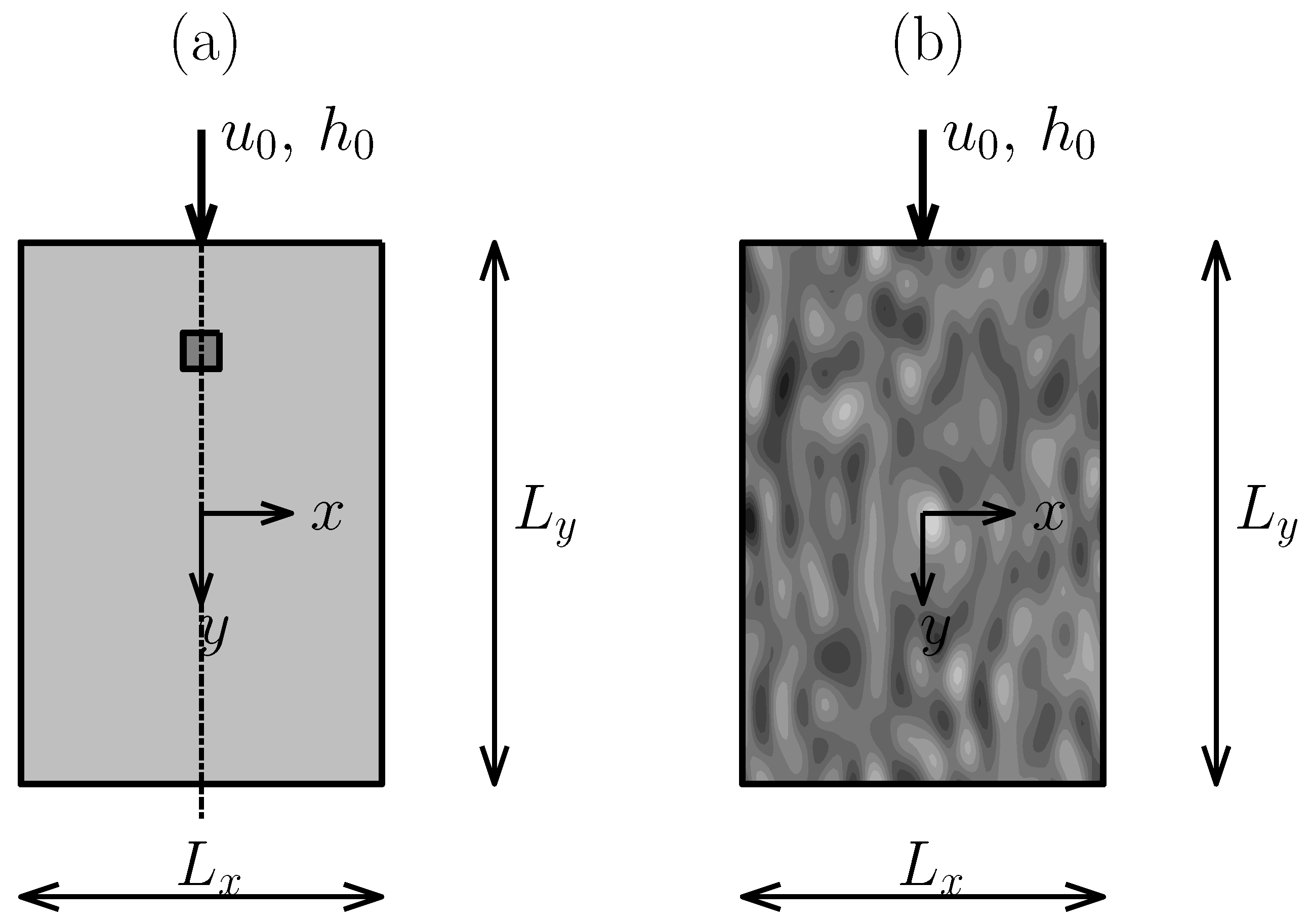
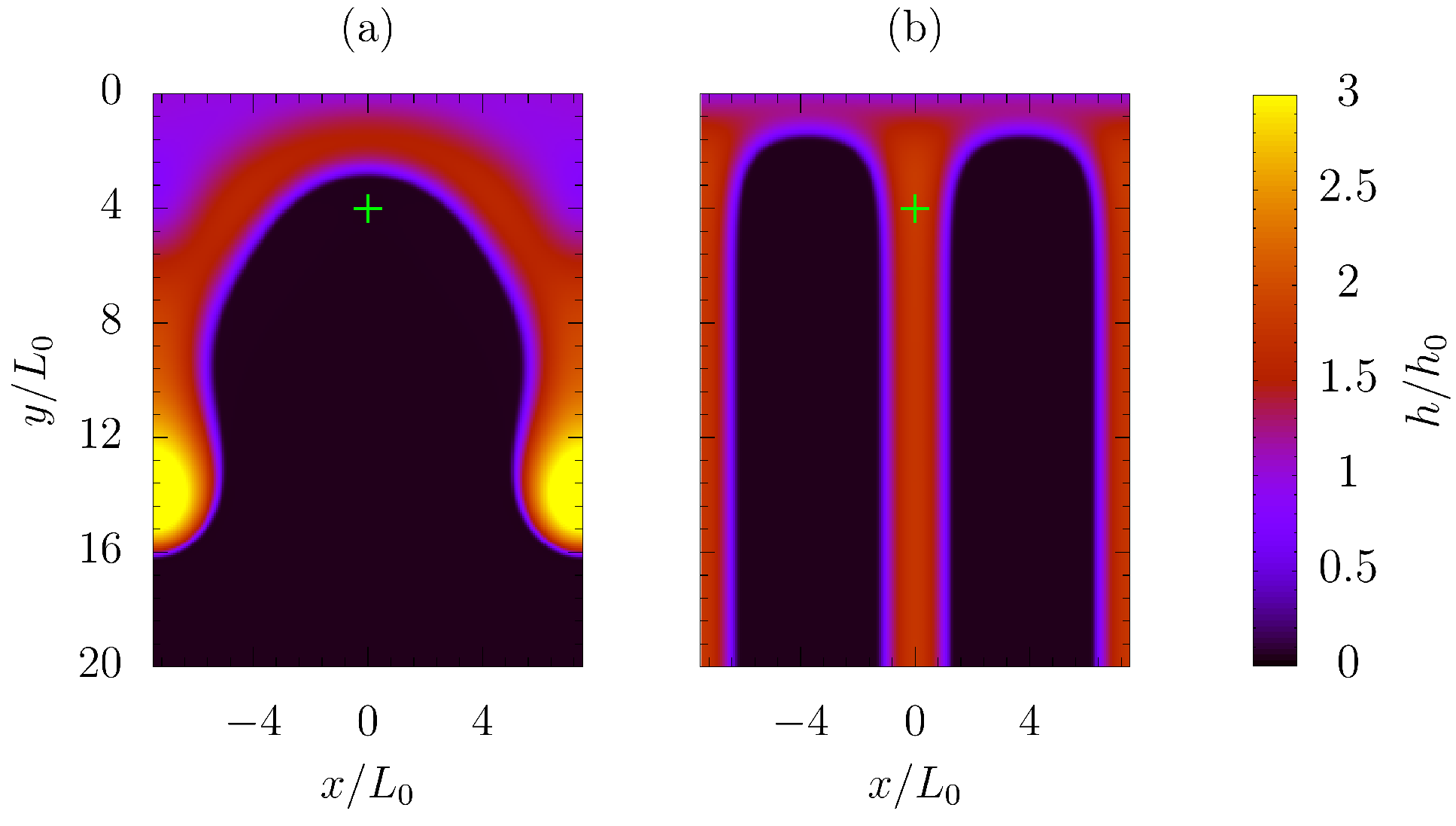
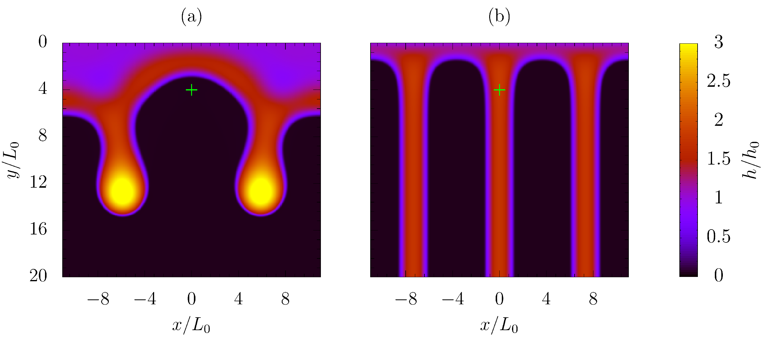
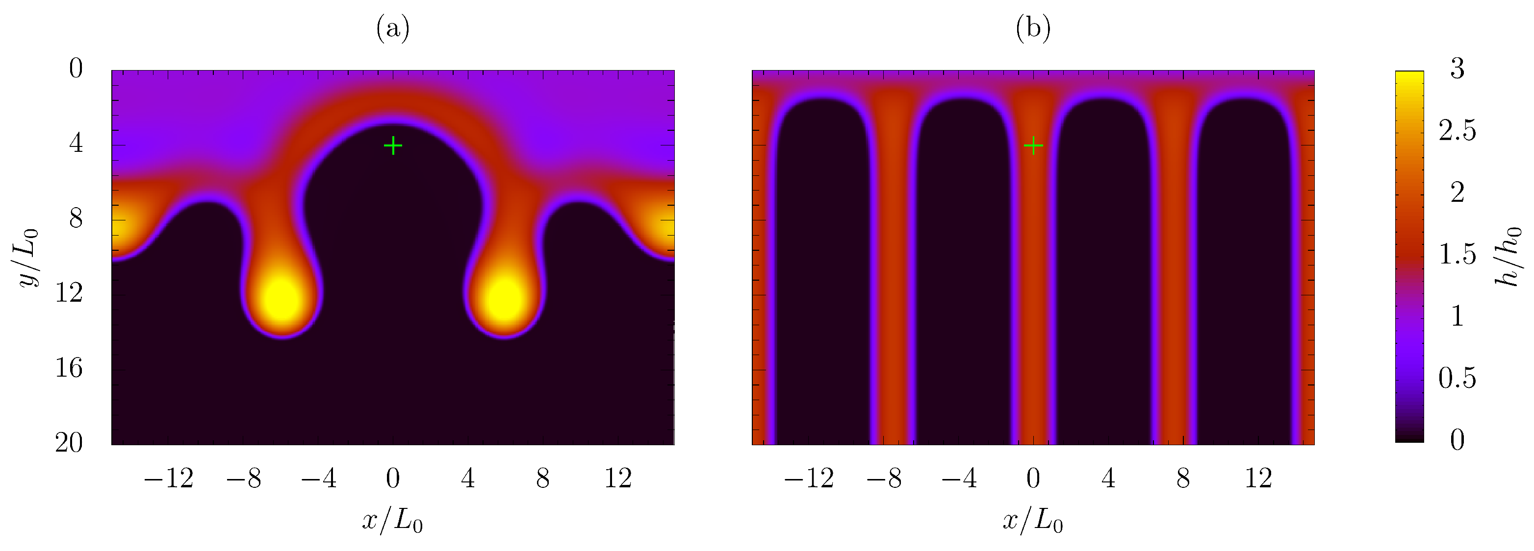
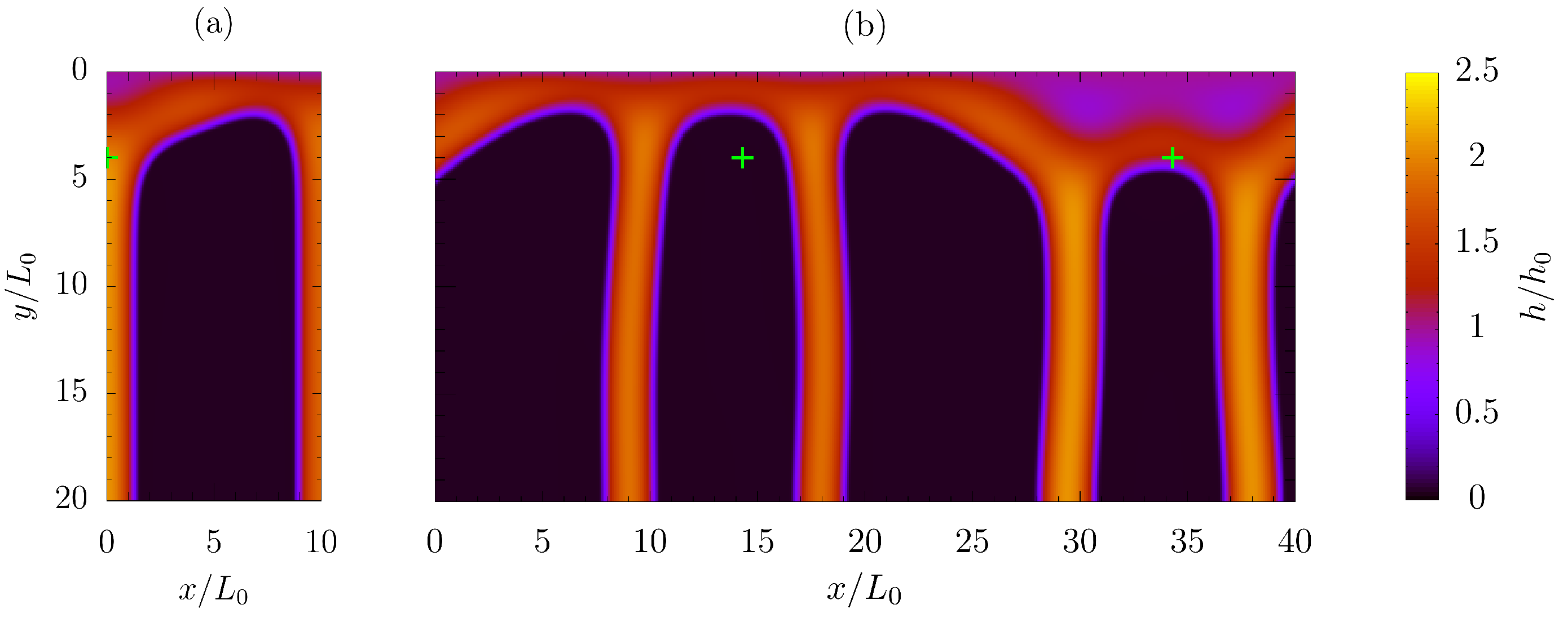
• Second, a 2D film flowing down an inclined plate, characterized by a single array of equally spaced contamination spots with decreased surface wettability, was simulated, Figure 1a. Defining $L_X$ as the distance between adjacent contamination spots, only a portion of width $L_X/2$ was considered, due to the problem symmetry. Thus, symmetry condition was imposed through $X=0$ and $X=L_X/2$, while inlet condition and fully developed flow were applied at $Y=0$ (top-most section) and $Y=L_Y$ (bottomest section) respectively. The low-wettable square patch of dimension $L_0$ defining the contamination spot was located at $Y=4$, far enough from the inlet section ($Y=0$) to avoid boundary effects.
• Finally, the hybrid surface shown in Figure 1b, characterized by the following periodic, isotropic smooth random wettability distribution from [26], was investigated,

  $$\begin{array}{cc}\hfill & \theta (x,y)={\theta }_0+\sum _{k=-n_0}^{+n_0}\sum _{j=-m_k}^{+m_k}{a}_{j,k}cos\left(\frac{2\pi jx}{L_x}+\frac{2\pi ky}{L_y}+{\psi }_{j,k}\right)\hfill \end{array}$$

  (21)

  $$\begin{array}{cc}\hfill & m_k=⌊m_0\sqrt{1-{\left(\frac{k}{n_0}\right)}^2}⌋,\hfill \end{array}$$

  (22)

  with $a_{jk}$ being random coefficients falling inside a given range, ${\psi }_{j,k}\in \left[-\pi ,+\pi \right]$ being the random phase of cosine function, $m_0$ and $n_0$ being the number of harmonics over x and y. In order to ensure physical consistency, periodic conditions were applied through $X=0$ and $X=L_X$. Inlet condition and fully developed flow were again applied through $Y=0$ and $Y=L_Y$.

The solution was always initialized imposing a dry domain, i.e., assuming a uniform film thickness, equal to the characteristic precursor film over the whole computational domain at the initial stage of the computation, ${\left.H(X,Y)\right|}_{T_0}=\delta$.

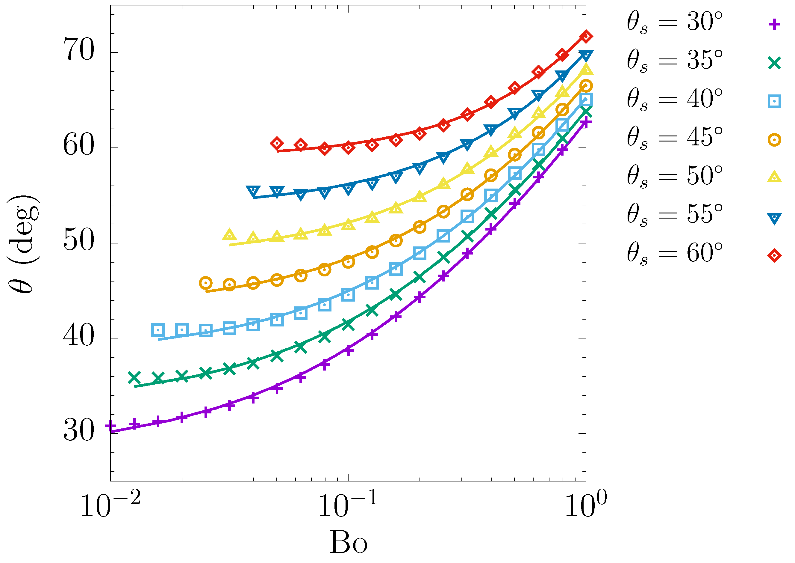
3.2. Dynamic Contact Angle

The stability of a 1D film falling down an inclined plate was investigated, running parametric computations at decreasing film Bond number, until film rupture was observed. Different surface wettabilities were investigated, with the imposed contact angle varying in the wider range allowed by the full free surface curvature formulation, ${\theta }_s\in \left[{30}^{\circ },{60}^{\circ }\right]$. The plate slope was set to $\alpha ={60}^{\circ }$ for all the simulations. The dynamic (advancing) contact angle $\theta$, computed as the maximum free surface slope at the apparent contact line, was also traced, in case of a stable film, for each computation, considering the self-similar free surface profile of the advancing film. According to literature [12,13,18,20], the precursor film thickness and the disjoining exponents were set to $\delta =5\times {10}^{-2}$ and $n=3,m=2$, which represents a good compromise between computational costs and accuracy of the numerical solution. A preliminar grid independency analysis was conducted in the most critical configuration. Thus, setting ${\theta }_s={60}^{\circ }$, $Bo=5\times {10}^{-2}$, which represents one of the most critical investigated configurations, and progressively decreasing the spatial discretization step $\Delta X$, it was found that $\Delta X=1.5\times {10}^{-2}$ ensures grid independency, since further decreasing $\Delta X$ to $7.5\times {10}^{-3}$ leads to a less than $1\%$ deviation on the computed dynamic contact angle. Thus, a spatial discretization step of $\Delta X\le 1.5\times {10}^{-2}$ was imposed for all the computations.

In Figure 2a, both the stable film solution and the self-similar droplet deriving from film rupture are presented for a given surface wettability, ${\theta }_s={60}^{\circ }$, and slightly different Bond numbers. A bifurcation of the solution is, thus, observed as the stable film configuration is replaced, below the critical Bond number, by the droplet regime, induced by film rupture occurrence. Figure 2b shows the stable film solution at $Bo=5.01$, but different surface wettabilities, qualitatively demonstrating that higher free surface slope, are obtained by imposing higher static contact angle in the disjoining pressure.

The dynamic contact angle, traced as a function of both the surface wettability and the Bond number in case of a stable advancing 1D film, is presented in Figure 3. It is worth pointing out that the critical Bond number, which defines the transition between film instability occurrence and stable film (leftmost markers in Figure 3), depends on the imposed surface wettability, with a higher contact angle leading to higher critical Bond number (thus, the film is likely to be subject to instability phenomena at lower surface wettability). As widely reported in literature [12,27,28], the cube of the dynamic contact angle depends on the film velocity according to Tanner–Hoffman–Voinov law,

$${\left(\frac{\theta }{{\theta }_s}\right)}^3=1+C\frac{\mu u_c}{\sigma },u_c=u_0\frac{1-{\delta }^3}{1-\delta },$$

(23)

with $u_0$ being the undisturbed film velocity and C being a constant parameter. Expressing $u_0$ via Nusselt film theory, Equation (1), and retaining the usually neglected logarithmic term [28], Equation (23) can be recast as

$${\left(\frac{\theta }{{\theta }_s}\right)}^3=C_0+Bo\left[C_1+C_{2}log\left({Bo}^{1/3}\right)\right].$$

(24)

Following [19,20], the computed dynamic contact angle is compared to Equation (24), with $C_{0,1,2}$ being the fitting parameters, in order to verify the effectiveness of disjoining pressure model in the wider range of contact angles allowed by the full curvature formulation. Almost a perfect agreement for ${\theta }_s$ up to ${60}^{\circ }$ can be observed in Figure 3.

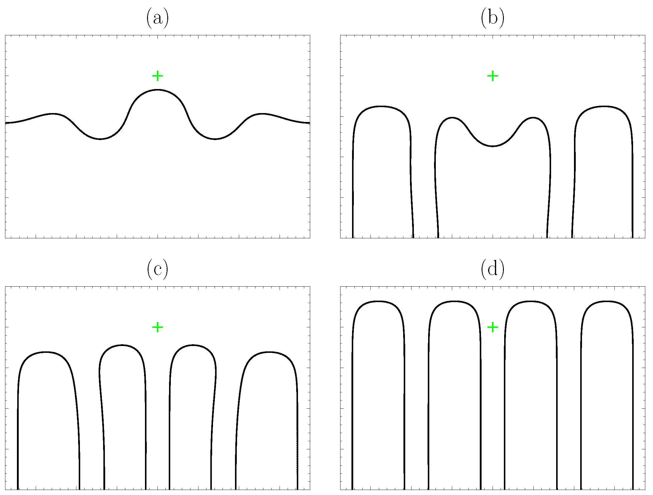
3.3. Single Array of Contamination Spots

A single array of lower wettability contamination spots, characterized by an increased value of the imposed static contact angle, was investigated, as pointed out in Section 3.1. A somewhat similar setup was investigated by Zhao and Marshall [12], who imposed a sequence of vertical strips, with different contact angle inducing fingering instability. Here, the eventual film instability is induced by localized spots. Furthermore, higher contact angles are here investigated, as allowed by the full modelization of the free surface curvature. The influence of both the dimensionless distance $L_X$ between successive contamination spots and the film Bond number, Equation (10), on the resulting liquid layer distribution were analysed, in terms of number of observed rivulets. Parametric computations were run, in the range $L_X\in [5,30]$ and $Bo\in [0.11,0.16]$. The static contact angle was set to ${\theta }_s={60}^{\circ }$ over the whole computational domain, except inside the contamination spot, where the contact angle was set to an increased value of ${75}^{\circ }$, while the plate slope was set to $\alpha ={60}^{\circ }$. According to literature [12,13,18,20], the precursor film thickness was set to $\delta =5\times {10}^{-2}$, while the disjoining exponents were set to $n=3$, $m=2$. Spatial discretization steps of $\Delta X,\Delta Y\le 1.5\times {10}^{-2}$ were imposed in order to ensure grid independency, while $L_Y=20$ was chosen as the plate length along the downhill direction, in order to let the liquid film develop and, thus, avoid boundary effects.

All the observed configurations, defined by the number of rivulets flowing within a periodic length $L_X$, are summarized in the bifurcation diagram, Figure 4, as a function of the distance between neighbor contamination spots and of the Bond number. Figure 4a shows the number of rivulets at $T=10$ (thus, right after the undisturbed film gets over the contamination spots). Since the liquid bulk has not reached the outlet section at $T=10$, the number of rivulets was computed as the number of streamwise peaks of the evolving contact line, which is defined by the position of the local maximum of the free surface slope. It is important to point out that the number of observed rivulets mainly depends on the dimensionless distance between neighbor contamination spots, which in turn depends on the imposed film Bond number,

$$L_X=\frac{L_x}{L_0}=\frac{L_x}{h_0}{Bo}^{1/3}.$$

(25)

In fact, critical lengths defining the transition between different configurations can be identified: $L_{01}\sim 6$ corresponds to the appearance of a single rivulet; $L_{12}\sim 16$ defines the transition from 1 to 2 rivulets; $L_{23}\sim 25$ defines the transition between 2 to 3 rivulets. Additionally, defining $\Delta L_1=L_{12}-L_{01}$ and $\Delta L_2=L_{23}-L_{12}$, it comes that new rivulets forms at $\Delta L_i$ close to the characteristic perturbation wavelength, $\lambda =9.4$, deriving from linear stability analysis of the governing lubrication equation [12].

The above defined instabilities may evolve into stable dry patches or may be shed away, leaving a continuous film upstream of an advancing unstable front. These regimes are mapped in Figure 4b, which depicts the steady state solution. The figure offers a complex behavior, since it includes long term evolution and effective growth of the local perturbance, and the effect of the imposed restrictions (such as periodicity) which are not accounted for in the linear stability analysis. Figure 4b shows that five different configurations can be observed: fully wetted domain ($N=0$), usually observed at low distance between neighbor low-wettable spots and at high Bond number; a single rivulet ($N=1$), which flows between neighbor contamination spots; 2 rivulets ($N=2$), one flowing between neighbor contamination spots and one wetting the contamination spot, as shown by Figure 5b; 3 rivulets ($N=3$), 2 of them forming between neighbor contamination spots and one wetting the spot, Figure 6b; 4 rivulets ($N=4$), 3 between neighbor contamination spots and, again, one more rivulet, which wets the spot, Figure 7b.

Figure 5, Figure 6 and Figure 7, which show some of the observed configurations at $Bo=0.11$ and increasing distance $L_X$ between contamination spots, apparently suggest a correlation between the dimensionless length $L_X$ (which is, in turn, correlated to the number of transient rivulets, observed right after the liquid front hits the contamination spot) and the number of steady rivulets. However, looking at Figure 4b, both the 3 rivulets and the fully wetted configurations may occur at an unexpected high value of $L_X$.

For a better understanding of the contact line dynamics, different screenshots of the moving contact line are taken from two different computations at $Bo=0.11$ and slightly different $L_X$. In Figure 8, which refers to the same test case as Figure 7, $L_X=30$, the contact line position is traced at successive instants: 3 rivulets have already formed at $T=10$, Figure 8a; after the rivulets develop and become narrow, there is enough space for one more rivulet front to form below to the contamination spot and drain, Figure 8b,c; as long as the generated dry patches are stable, all the rivulets just settle down and remain as stationary rivulets, Figure 8d.

The moving contact line was traced, at the same instants, during a computation at slightly different distance between contamination spots, $L_X=27$: similarly to the previous case ($L_X=30$), 3 rivulets forms after the liquid front meets the contamination spot, Figure 9a; again, after the rivulets settle down, a new rivulet front forms below the contamination spot, Figure 9b; however, the dry patches, induced by the formation of the new, central rivulet, slowly moves downstream, generating a bottle-neck shape that evolves in a single rivulet, Figure 9c; thus, only 2 stationary rivulets are observed, Figure 9d. Furthermore, one of the stable rivulets is larger then the other one, since it collects the liquid flux of the three original rivulets that moved downstream, out of the computational domain. A similar behavior was observed, at $Bo=0.11$, when $L_X=21$, with dry patch closure phenomenon that leads to only 2 stable rivulets, while 3 rivulets can be observed, when $L_X=22$, in Figure 6b. When fully wetted condition is detected, as it happens for $Bo=0.11$ and $L_X=20$, the liquid front simply overtakes the contamination spot.

Fully wetted condition is progressively incentivated at higher Bond number, see Figure 4b, as the gravitational force dominates the surface tension, ensuring stability of the liquid film. However, it is quite interesting for practical applications, which often requires the existence of stable and thin films at dominating surface tension forces, that the fully wetted condition can be obtained even at the lower Bond numbers, under restricted geometrical characteristics of the solid surface.

In order to test the consistency of the applied boundary conditions (i.e., half of the periodic length investigated, contamination spot located at $X=0$ and symmetry conditions applied to $X=0$ and $X=L_X$), a larger domain of width $2L_X$ (thus, including 2 contamination spots, located at $X=14.3,34.3$) with periodic conditions, applied through $X=0$ and $X=2L_X$, was also simulated. In fact, the latter test case allows the film to evolve in a larger domain (4 times the characteristic perturbation length ${\lambda }_{cr}$ from linear theory), mitigating the artificial constraints deriving from forcing the film to follow the geometrical symmetry. A configuration characterized by low Bond number, $Bo=0.10$, giving a film subject to instability phenomena even when weak perturbations are introduced, was considered. As demonstrated by Figure 10, which shows the liquid layer distribution resulting from the two different computations at the same instant $T=125$, the same number of rivulets per unit length is predicted, meaning that the results proposed in the bifurcation diagram, Figure 4b, are statistically consistent, although the solution is less regular and may also have some oscillations in time.

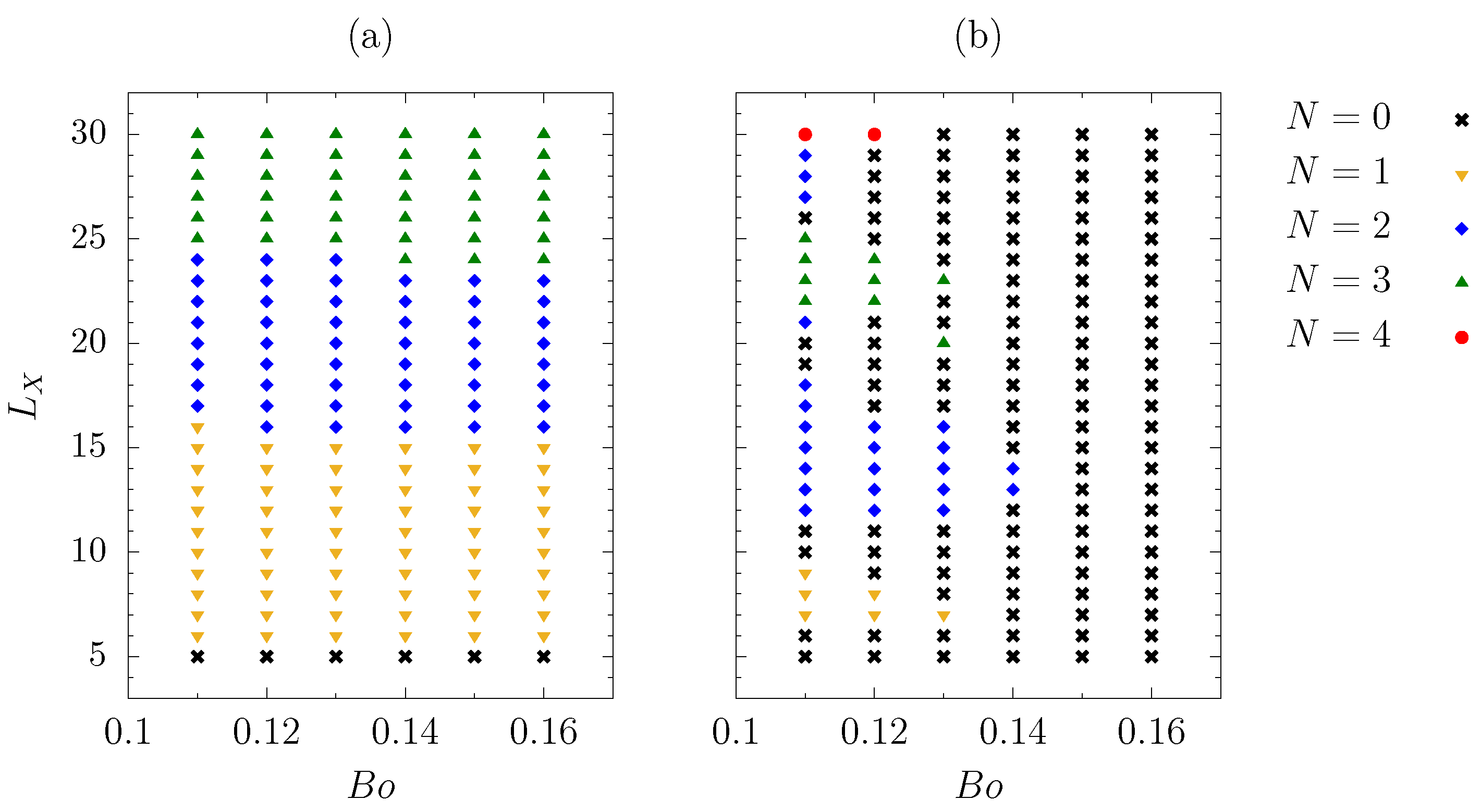
3.4. Randomly Generated Heterogeneous Surface

A general heterogeneous surface, characterized by a random, periodic distribution of the static contact angle, implemented through Equation (21), was also investigated. Such a test case is aimed to mimic the typical surfaces occurring in practical application. A large computational domain, characterized by $L_X=40$ and $L_Y=50$, was considered in order to let the induced perturbance grow without any numerical constraint. The plate slope and the Bond number were set to $\alpha ={60}^{\circ }$ and $Bo=0.1$, while the static contact angle was ranged in ${\theta }_s\in [{45}^{\circ },{60}^{\circ }]$ over the heterogeneous surface. The characteristics of the heterogeneous surface are imposed through the number of harmonics $(m_0,n_0)$ considered in Equation (21), which defines the wavelength parameters, ${\Lambda }_X=L_X/m_0$, ${\Lambda }_Y=L_Y/n_0$: in order to ensure isotropy, $\Lambda ={\Lambda }_X={\Lambda }_Y$ was always imposed. The precursor film thickness and the disjoining exponents were again set to $\delta =5\times {10}^{-2}$ and $n=3,m=2$. A spatial discretization step of $\Delta X,\Delta Y\le 2.5\times {10}^{-2}$ was imposed in order to ensure grid independency. Parametric computations were run at different values of the characteristic length $\Lambda$, defining the random surface heterogeneity. The number of rivulets, generated due to finger instability induced by the random contact angle distribution, was then traced at $T=25$, in order to statistically investigate the effect of the heterogeneous surface characteristics on the liquid film evolution.

The hybrid surface wettability distributions at different magnitudes of $\Lambda$ are shown in Figure 11a,b, referred to $\Lambda =2\times {10}^{-2}$ and $\Lambda =2$, respectively. The corresponding film thickness distributions at $T=25$ are reported in Figure 12a,b. Fully wetted condition was observed at the end of both the computations. However, different behaviors were observed, with 4 rivulets obtained when $\Lambda =2\times {10}^{-2}$ and 3 rivulets obtained when $\Lambda =2$.

Table 1. Number of rivulets observed after $T=25$ and at steady state solution ($T\to \infty$) as a function of the characteristic length $\Lambda$ of the heterogeneous surface. $Bo=0.1$, ${\theta }_s\in \left[{45}^{\circ },{60}^{\circ }\right]$, $\alpha ={60}^{\circ }$, $L_X=40,L_Y=50$.

$\mathbf{\Lambda }$	${\mathit{m}}_0$	${\mathit{n}}_0$	${\mathit{N}}_{\mathbf{riv}}$
			$\mathbf{T}=\mathbf{25}$	$\mathbf{T}\to \infty$
$2\times {10}^{-1}$	200	250	4	0
$5\times {10}^{-1}$	80	100	3	0
1	40	50	3	0
2	20	25	3	0
5	8	10	3	0

, which reports the number of observed rivulets at $T=25$, reveals that a transition from 4 rivulets configuration to 3 rivulets occurs at $\Lambda \ge 5\times {10}^{-2}$. Fully wetted domain ($N_{riv}=0$ at $T\to \infty$ in Table 1) was obtained for all the investigated values of $\Lambda$. Thus, the dry patches induced by finger instability are shed away, leaving a continuous film upstream from the unstable advancing liquid front.

Thus, the linear theory, which gives a characteristic perturbation wavelength of ${\lambda }_{cr}=9.4$ (i.e., 4 rivulets in the investigated test cases), as expected does not provide the effective evolution of film instability induced by local perturbance (in turns given by surface heterogeneity) when the magnitude of the surface parameter $\Lambda$ is comparable to ${\lambda }_{cr}$, i.e., when the actual geometrical details of the perturbation affect contact line movement.

4. Conclusions

The enhanced lubrication equations were numerically solved. Contact angles up to ${60}^{\circ }$ (locally increased at ${75}^{\circ }$ inside localized, lower-wettable contamination spots) were investigated thanks to the full curvature formulation, which substitutes the usually adopted small slope approximation, leading to accurate results for ${\theta }_s<{30}^{\circ }$ [23]. Film rupture occurrence was analyzed for a 1D falling film. The computed, dynamic contact angle was successfully verified with the Hoffman–Voinov–Tanner law for ${\theta }_s$ up to ${60}^{\circ }$. Then, parametric computations were run for a 2D film over a heterogeneous surface. It was verified that the onset of finger instability, induced by an horizontal array of localized, lower wettable contamination spots with ${\theta }_s={75}^{\circ }$, follows the literature linear stability analysis. The long term evolution of the induced instability, affected by the imposed restrictions, was traced under different flow conditions and contamination spot spacing. A complex behavior, including multiple configurations (continuous film and 1 to 4 rivulet regimes), was observed due to the bifurcation occurrence. However, artificially controlling the solid surface morphology (i.e., the contamination spot spacing) allows to achieve the continuous film regime at given flow characteristics (i.e., required film thickness). This is crucial in practical applications, since the whole coverage of a solid surface can be ideally obtained at the lower film thickness (usually more subject to instability phenomena): in absorption/distillation through structured packing, a proper design of the packing geometry may lead to high liquid–gas interface area even at low film thickness, enhancing mass transfer and avoiding flooding condition inside structured packing. The flow down an inclined plate with random surface distribution, which mimics practical configurations, was also investigated: the liquid film behavior can no longer be predicted via linear stability analysis when the magnitude of the characteristic surface length is comparable to the perturbation length from linear theory. Finally, it is worth pointing out that the parallelization of the solver code allowed to speed up computations, while the implemented ADI factorization allowed to reach time integration step up to ${10}^8$ times the step size from Von Neumann stability analysis on the explicit numerical scheme.

References

1. Croce, G.; De Candido, E.; Habashi, W.G.; Munzar, J.; Aube, M.; Baruzzi, G.S.; Aliaga, C. FENSAP-ICE: Analytical model for spatial and temporal evolution of in-flight icing roughness. J. Aircr. 2010, 47, 1283–1289. [Google Scholar] [CrossRef]
2. Schweizer, P.M.; Kistler, S.F. Liquid Film Coating: Scientific Principles and Their Technological Implications; Springer: Berlin/Heidelberg, Germany, 2012. [Google Scholar]
3. Rocha, J.A.; Bravo, J.L.; Fair, J.R. Distillation Columns Containing Structured Packings: A Comprehensive Model for Their Performance. 1. Hydraulic Models. Ind. Eng. Chem. Res. 1993, 32, 641–651. [Google Scholar] [CrossRef]
4. Rocha, J.A.; Bravo, J.L.; Fair, J.R. Distillation Columns Containing Structured Packings: A Comprehensive Model for Their Performance. 2. Mass-Transfer Model. Ind. Eng. Chem. Res. 1996, 35, 1660–1667. [Google Scholar] [CrossRef]
5. Xie, Z.; Zhu, W. Theoretical and experimental exploration on the micro asperity contact load ratios and lubrication regimes transition for water-lubricated stern tube bearing. Tribol. Int. 2021, 164, 107105. [Google Scholar] [CrossRef]
6. Xie, Z.; Zhang, Y.; Zhou, J.; Zhu, W. Theoretical and experimental research on the micro interface lubrication regime of water lubricated bearing. Mech. Syst. Signal Process. 2021, 151, 107422. [Google Scholar] [CrossRef]
7. Wen, J.; Zhang, W.Y.; Ren, L.Z.; Bao, L.Y.; Dini, D.; Xi, H.D.; Hu, H.B. Controlling the number of vortices and torque in Taylor-Couette flow. J. Fluid Mech. 2020, 901, A30. [Google Scholar] [CrossRef]
8. Elmaboud, Y.A.; Abdelsalam, S.I. DC/AC magnetohydrodynamic-micropump of a generalized Burger’s fluid in an annulus. Phys. Scr. 2019, 94, 115209. [Google Scholar] [CrossRef]
9. Diez, J.A.; Kondic, L. Computing Three-Dimensional Thin Film Flows Including Contact Lines. J. Comput. Phys. 2002, 183, 274–306. [Google Scholar] [CrossRef] [Green Version]
10. Thiele, U.; Brusch, L.; Bestehorn, M.; Bar, M. Modelling thin-film dewetting on structured substrates and templates: Bifurcation analysis and numerical simulations. Eur. Phys. J. E 2003, 11, 255–271. [Google Scholar] [CrossRef]
11. Shkadov, V.Y.; Sisoev, G.M. Numerical bifurcation analysis of the travelling waves on a falling liquid film. Comput. Fluids 2005, 34, 151–168. [Google Scholar] [CrossRef]
12. Zhao, Y.; Marshall, J.S. Dynamics of driven liquid films on heterogeneous surfaces. J. Fluid Mech. 2006, 559, 355–376. [Google Scholar] [CrossRef]
13. Sellier, M. Modelling the wetting of a solid occlusion by a liquid film. Int. J. Multiph. Flow 2015, 71, 66–73. [Google Scholar] [CrossRef]
14. Wilson, S.K.; Duffy, B.R.; Davis, H. On a slender dry patch in a liquid film draining under gravity down an inclined plane. Eur. J. Appl. Math. 2001, 12, 233–252. [Google Scholar] [CrossRef] [Green Version]
15. Yatim, Y.M.; Duffy, B.R.; Wilson, S.K. Travelling-wave similarity solutions for a steadily translating slender dry patch in a thin fluid film. Phys. Fluids 2013, 25, 052103. [Google Scholar] [CrossRef] [Green Version]
16. Rio, E.; Limat, L. Wetting hysteresis of a dry patch left inside a flowing film. Phys. Fluids 2006, 18, 032102. [Google Scholar] [CrossRef]
17. Podgorski, T.; Flesselles, J.M.; Limat, L. Dry arches within flowing films. Phys. Fluids 1999, 11, 845. [Google Scholar] [CrossRef]
18. Schwartz, L.W.; Eley, R.R. Simulation of Droplet Motion on Low-Energy and Heterogeneous Surfaces. J. Colloid Interface Sci. 1998, 202, 173–188. [Google Scholar] [CrossRef]
19. Suzzi, N.; Croce, G. Numerical simulation of rivulet build up via lubrication equations. J. Phys. Conf. Ser. 2017, 923, 012020. [Google Scholar] [CrossRef]
20. Suzzi, N.; Croce, G. Numerical simulation of film instability over low wettability surfaces through lubrication theory. Phys. Fluids 2019, 31, 122106. [Google Scholar] [CrossRef]
21. Suzzi, N.; Croce, G. Bifurcation analysis of liquid films over low wettability surfaces. J. Phys. Conf. Ser. 2021, 1868, 012010. [Google Scholar] [CrossRef]
22. Nusselt, W. Die oberflächenkondensation des wasserdampfes. Z. Ver. Deutsch. Ing. 1916, 60, 569–575. [Google Scholar]
23. Perazzo, C.A.; Gratton, J. Navier-Stokes solutions for parallel flow in rivulets on an inclined plane. J. Fluid Mech. 2004, 507, 367–379. [Google Scholar] [CrossRef]
24. Do Carmo, M.P. Differential Geometry of Curves and Surfaces; Pearson: New York, NY, USA, 1976; p. 163. [Google Scholar]
25. Witelski, T.P.; Bowen, M. ADI schemes for higher-order nonlinear diffusion equations. Appl. Numer. Math. 2003, 45, 331–351. [Google Scholar] [CrossRef]
26. Filip, S.I.; Javeed, A.; Trefethen, L.N. Smooth random functions, random ODEs, and Gaussian processes. SIAM Rev. 2019, 61, 185–205. [Google Scholar] [CrossRef] [Green Version]
27. Blake, T.D. The physics of moving wetting lines. J. Colloid Interface Sci. 2006, 299, 1–13. [Google Scholar] [CrossRef] [PubMed]
28. Ajaev, V.S. Coating Flows and Contact Line Models. In Interfacial Fluid Mechanics: A Mathematical Modeling Approach; Springer: Berlin/Heidelberg, Germany, 2012; pp. 39–69. [Google Scholar]
Figure 1. Investigated hybrid configurations: single array of equally spaced contamination spots (a); draft of the hybrid surface characterized by randomly distributed contamination spots (b).
Fluids 06 00405 g001
Figure 2. Stable film solution (continuous line) and self-similar droplet (dashed line) generated by film rupture at slightly different Bond numbers, θ s = 60 (a); Stable film solution at different surface wettabilities, B o = 5.01 (b). α = 60 .
Fluids 06 00405 g002
Figure 3. Dynamic contact angle for a stable film as a function of the film Bond number and of the static contact angle: numerical points (markers) vs. Equation (24) (continuous lines). Left-most markers depicts the critical Bond number at different surface wettability, below witch film instability occurs. 1D falling film, α = 60 .
Fluids 06 00405 g003
Figure 4. Bifurcation diagram with number of observed rivulets: number of rivulets at T = 10 (a); number of stationary rivulets (b). α = 60 , θ s = 60 ( 75 inside contamination spot).
Fluids 06 00405 g004
Figure 5. Film thickness solution at T = 11 (a); 2 rivulet configuration, steady state film distribution (b). B o = 0.11 , L X = 15 , α = 60 , θ s = 60 ( 75 inside contamination spot, denoted by a green cross).
Fluids 06 00405 g005
Figure 6. Film thickness solution at T = 11 (a); 3 rivulet configuration, steady state film distribution (b). B o = 0.11 , L X = 22 , α = 60 , θ s = 60 ( 75 inside contamination spot, denoted by a green cross).
Fluids 06 00405 g006
Figure 7. Film thickness solution at T = 11 (a); 4 rivulet configuration, steady state film distribution (b). B o = 0.11 , L X = 30 , α = 60 , θ s = 60 ( 75 inside contamination spot, denoted by a green cross).
Fluids 06 00405 g007
Figure 8. Moving contact line at T = 10 (a), T = 20 (b), T = 30 (c), and T = 75 (d). L X = 30 , θ s = 60 ( 75 inside contamination spot, denoted by a green cross).
Fluids 06 00405 g008
Figure 9. Moving contact line at T = 10 (a), T = 20 (b), T = 30 (c), and T = 150 (d). L X = 27 , θ s = 60 ( 75 inside contamination spot, denoted by a green cross).
Fluids 06 00405 g009
Figure 10. Numerical film thickness solution at T = 125 : half periodic length with symmetry boundary conditions through X = 0 and X = L X / 2 (a); larger computational domain, including 2 contamination spots, with periodic boundary condition through X = 0 and X = 2 L X (b). B o = 0.1 , L X = 20 , θ s = 60 ( 75 inside the contamination spot), α = 60 .
Fluids 06 00405 g010
Figure 11. Zoom of the static contact angle distribution over the randomly generated heterogeneous surfaces, Equation (21): Λ = 2 × 10 1 (a); Λ = 2 (b).
Fluids 06 00405 g011
Figure 12. Film thickness solution at T = 25 : Λ = 2 × 10 1 (a); Λ = 2 (b). B o = 10 1 , θ s 45 , 60 , α = 60 .
Fluids 06 00405 g012