
Computational Study of the Dynamics of the Taylor Bubble


Abstract
:1. Introduction
2. The Problem Formulation
3. Governing Equations and the Numerical Method
4. Simulation Results: Axially Symmetric Motion
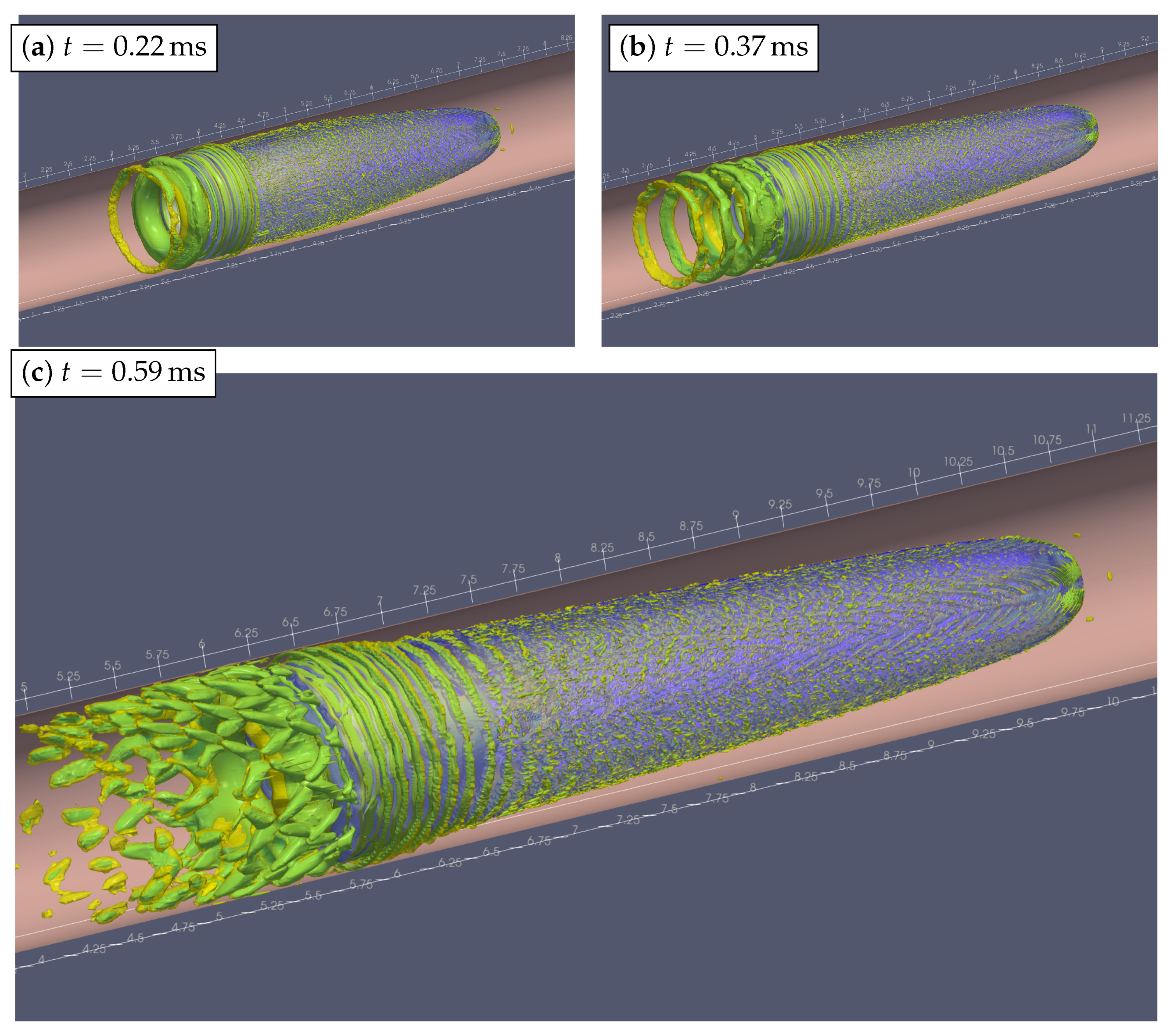
4.1. The Bubble Shape
4.2. Film Thickness and Its Dynamics
4.3. Bubble Velocity and Its Oscillations
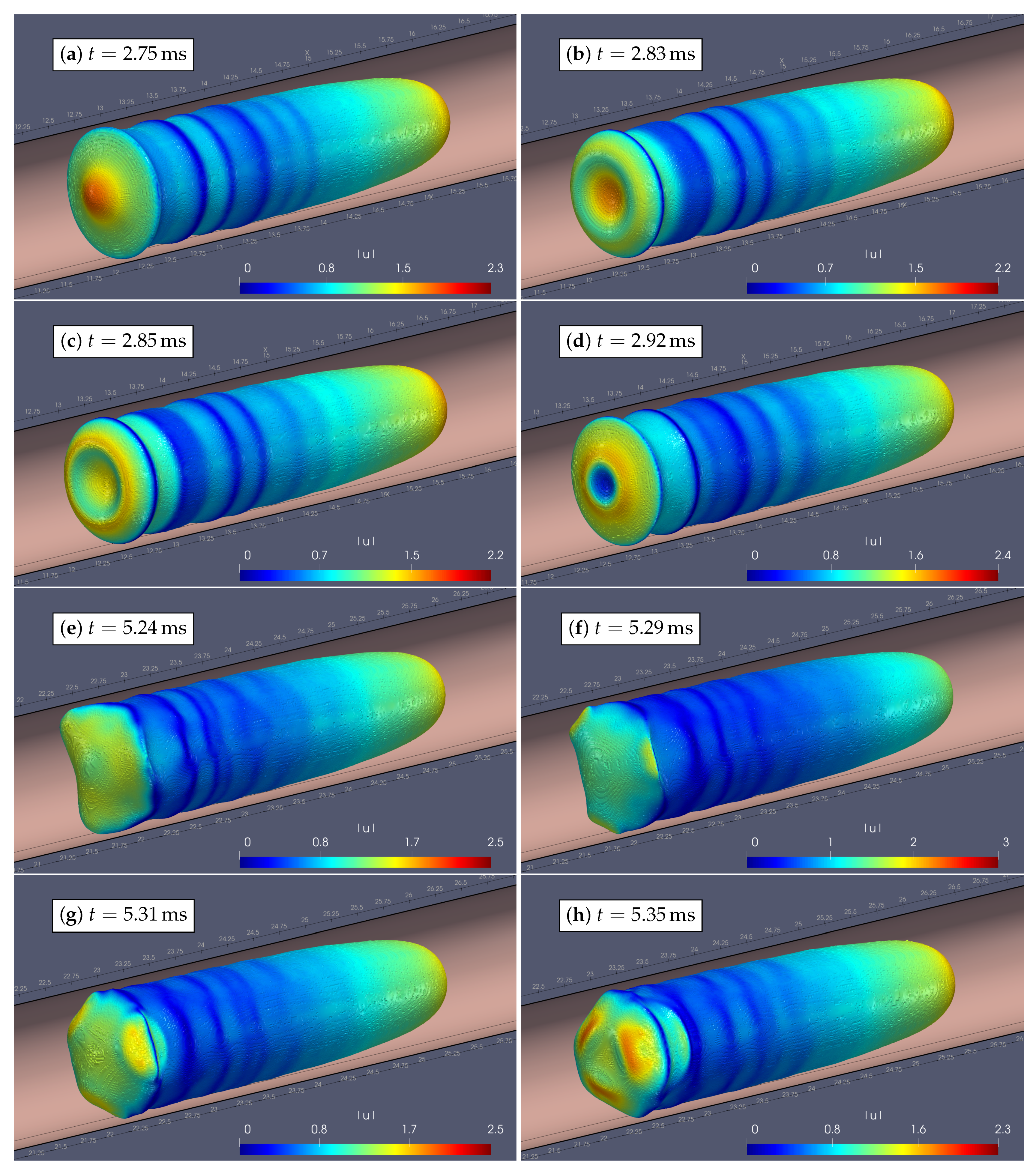
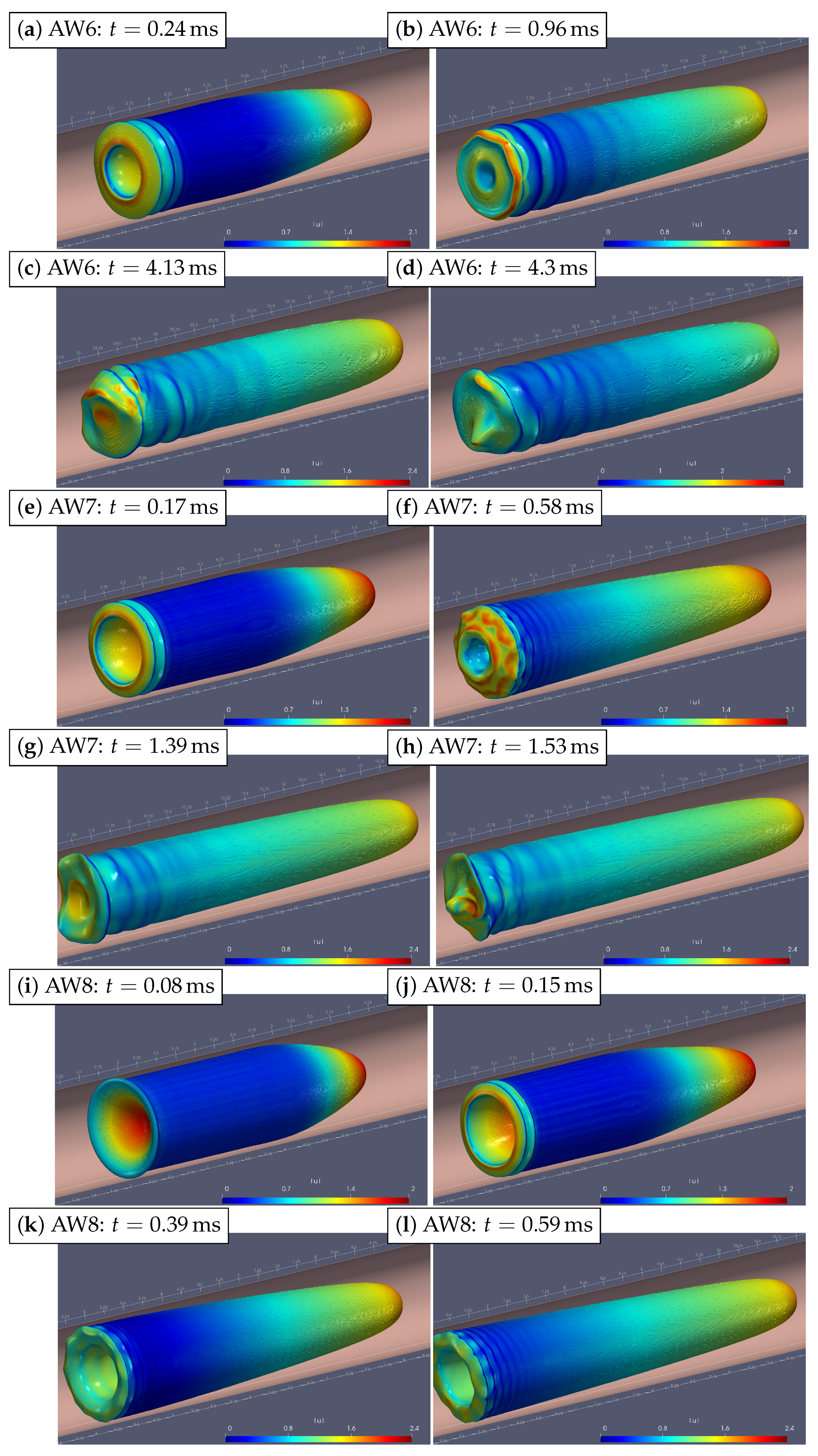
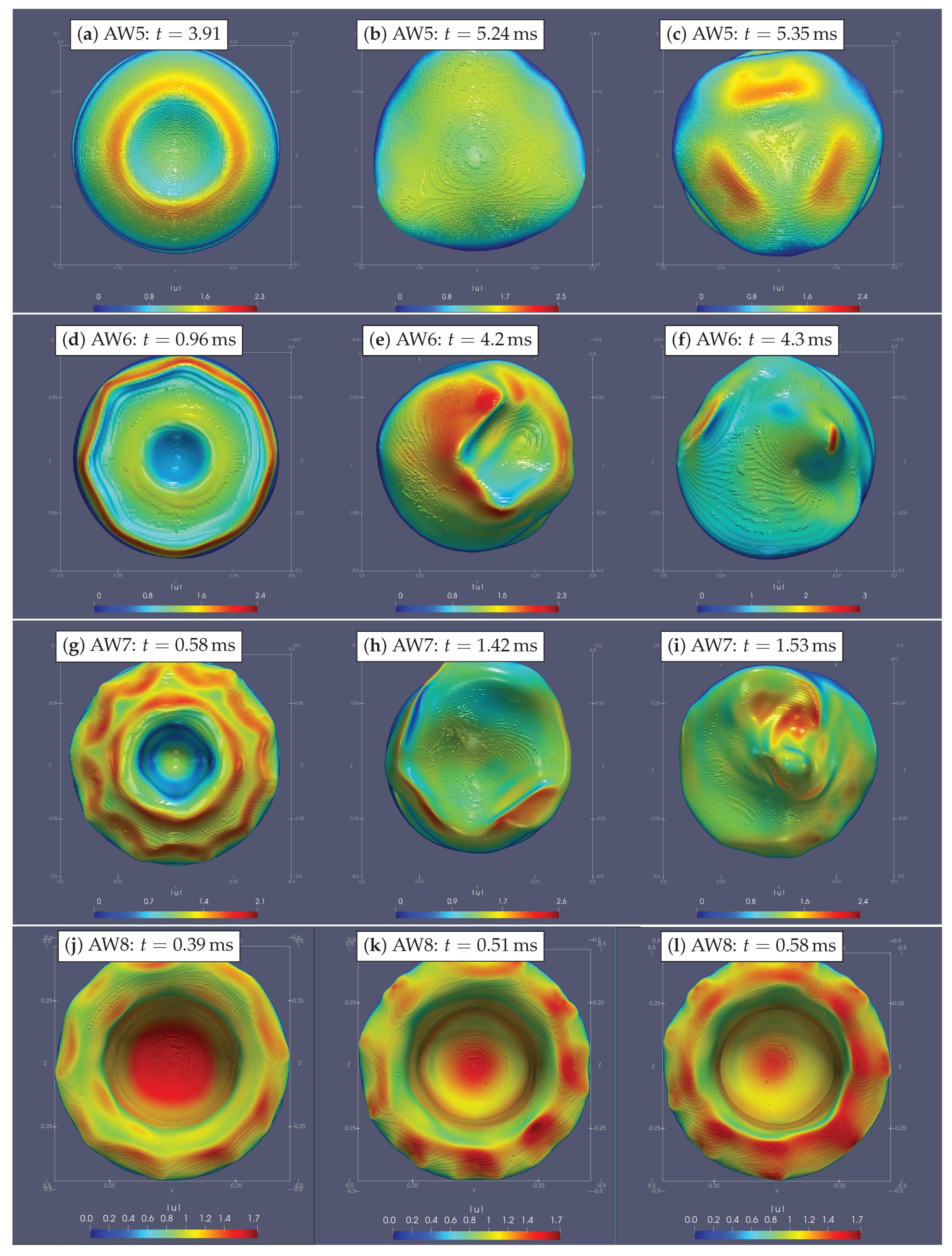
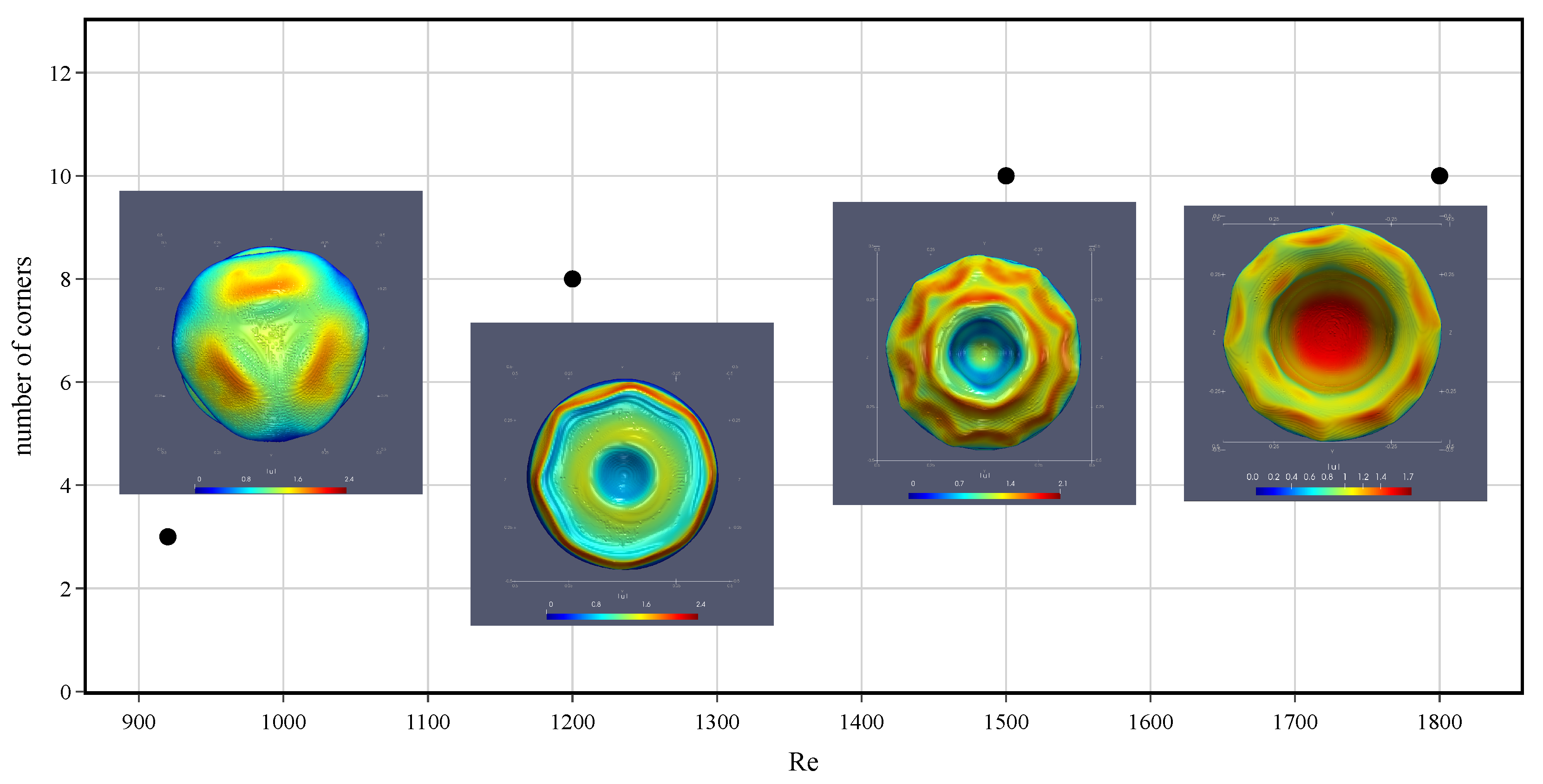
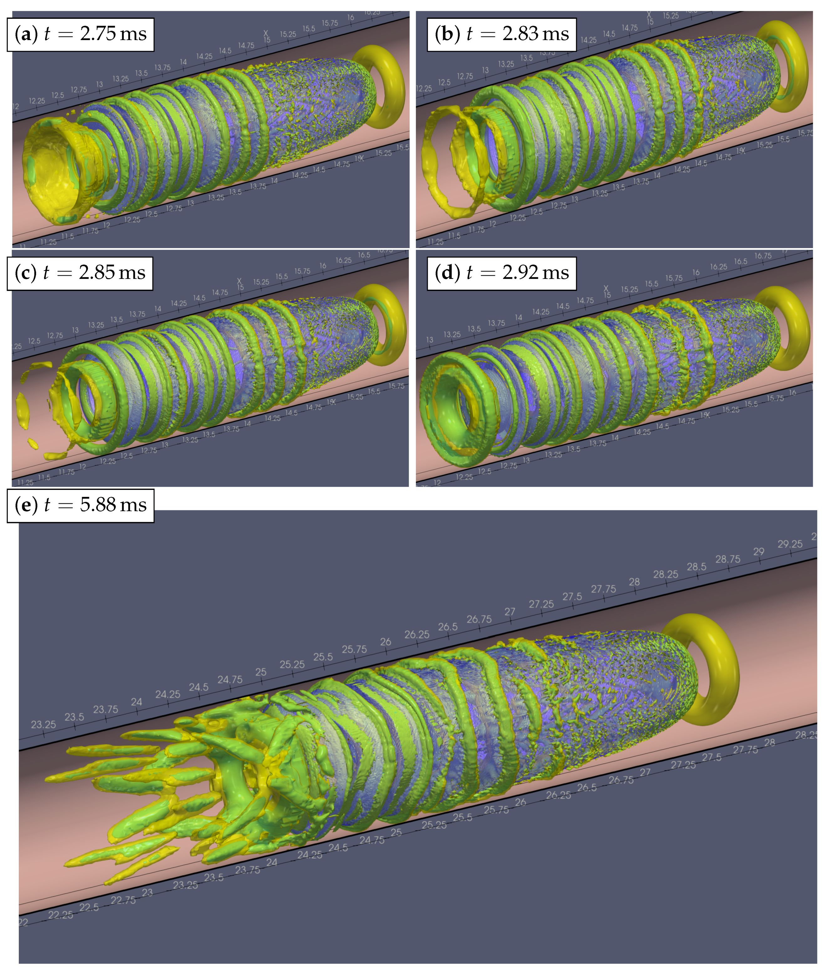
5. Simulation Results: Breaking of Axial Symmetry
Vortical Structures
6. Conclusions
Supplementary Materials
Author Contributions
Funding
Institutional Review Board Statement
Informed Consent Statement
Data Availability Statement
Acknowledgments
Conflicts of Interest
References
- Gravesen, P.; Branebjerg, J.; Jensen, O.S. Microfluidics-a review. J. Micromech. Microeng. 1993, 3, 168. [Google Scholar] [CrossRef]
- Zhang, J.; Yan, S.; Yuan, D.; Alici, G.; Nguyen, N.T.; Warkiani, M.E.; Li, W. Fundamentals and applications of inertial microfluidics: A review. Lab Chip 2016, 16, 10–34. [Google Scholar] [CrossRef] [PubMed] [Green Version]
- Shang, L.; Cheng, Y.; Zhao, Y. Emerging droplet microfluidics. Chem. Rev. 2017, 117, 7964–8040. [Google Scholar] [CrossRef] [PubMed]
- Anna, S.L. Droplets and bubbles in microfluidic devices. Annu. Rev. Fluid Mech. 2016, 48, 285–309. [Google Scholar] [CrossRef]
- Le, N.N.H.; Sugai, Y.; Nguele, R.; Sreu, T. Bubble size distribution and stability of CO2 microbubbles for enhanced oil recovery: Effect of polymer, surfactant and salt concentrations. J. Dispers. Sci. Technol. 2021, 42, 1974873. [Google Scholar]
- Grotberg, J.B. Respiratory fluid mechanics and transport processes. Annu. Rev. Biomed. Eng. 2001, 3, 421–457. [Google Scholar] [CrossRef] [PubMed]
- Yang, Y.; Chen, Y.; Tang, H.; Zong, N.; Jiang, X. Microfluidics for biomedical analysis. Small Methods 2020, 4, 1900451. [Google Scholar] [CrossRef]
- Sackmann, E.K.; Fulton, A.L.; Beebe, D.J. The present and future role of microfluidics in biomedical research. Nature 2014, 507, 181–189. [Google Scholar] [CrossRef]
- Rodríguez-Rodríguez, J.; Sevilla, A.; Martínez-Bazán, C.; Gordillo, J.M. Generation of microbubbles with applications to industry and medicine. Annu. Rev. Fluid Mech. 2015, 47, 405–429. [Google Scholar] [CrossRef]
- Dang, B.; Bakir, M.S.; Sekar, D.C.; King, C.R., Jr.; Meindl, J.D. Integrated microfluidic cooling and interconnects for 2D and 3D chips. IEEE Trans. Adv. Packag. 2010, 33, 79–87. [Google Scholar] [CrossRef]
- van Erp, R.; Soleimanzadeh, R.; Nela, L.; Kampitsis, G.; Matioli, E. Co-designing electronics with microfluidics for more sustainable cooling. Nature 2020, 585, 211–216. [Google Scholar] [CrossRef]
- Gilmore, N.; Timchenko, V.; Menictas, C. Microchannel cooling of concentrator photovoltaics: A review. Renew. Sustain. Energy Rev. 2018, 90, 1041–1059. [Google Scholar] [CrossRef]
- Bojang, A.A.; Wu, H.S. Design, fundamental principles of fabrication and applications of microreactors. Processes 2020, 8, 891. [Google Scholar] [CrossRef]
- Song, H.; Chen, D.L.; Ismagilov, R.F. Reactions in Droplets in Microfluidic Channels. Angew. Chem. Int. Ed. 2006, 45, 7336–7356. [Google Scholar] [CrossRef] [Green Version]
- Tanimu, A.; Jaenicke, S.; Alhooshani, K. Heterogeneous catalysis in continuous flow microreactors: A review of methods and applications. Chem. Eng. J. 2017, 327, 792–821. [Google Scholar] [CrossRef]
- Bandara, T.; Nguyen, N.T.; Rosengarten, G. Slug flow heat transfer without phase change in microchannels: A review. Chem. Eng. Sci. 2015, 126, 283–295. [Google Scholar] [CrossRef] [Green Version]
- Nirmal, G.M.; Leary, T.F.; Ramachandran, A. Mass transfer dynamics in the dissolution of Taylor bubbles. Soft Matter 2019, 15, 2746–2756. [Google Scholar] [CrossRef]
- Fletcher, D.F.; Haynes, B.S. CFD simulation of Taylor flow: Should the liquid film be captured or not? Chem. Eng. Sci. 2017, 167, 334–335. [Google Scholar] [CrossRef]
- Taylor, G.I. Deposition of a viscous fluid on the wall of a tube. J. Fluid Mech. 1961, 10, 161–165. [Google Scholar] [CrossRef]
- Bretherton, F.P. The motion of long bubbles in tubes. J. Fluid Mech. 1961, 10, 166–188. [Google Scholar] [CrossRef]
- Aussillous, P.; Quéré, D. Quick deposition of a fluid on the wall of a tube. Phys. Fluids 2000, 12, 2367–2371. [Google Scholar] [CrossRef]
- Han, Y.; Shikazono, N. Measurement of the liquid film thickness in micro tube slug flow. Int. J. Heat Fluid Flow 2009, 30, 842–853. [Google Scholar] [CrossRef]
- Khodaparast, S.; Magnini, M.; Borhani, N.; Thome, J.R. Dynamics of isolated confined air bubbles in liquid flows through circular microchannels: An experimental and numerical study. Microfluid. Nanofluidics 2015, 19, 209–234. [Google Scholar] [CrossRef]
- Rosengarten, G.; Harvie, D.; Cooper-White, J. Contact angle effects on microdroplet deformation using CFD. Appl. Math. Model. 2006, 30, 1033–1042. [Google Scholar] [CrossRef]
- Magnini, M.; Ferrari, A.; Thome, J.R.; Stone, H.A. Undulations on the surface of elongated bubbles in confined gas-liquid flows. Phys. Rev. Fluids 2017, 2, 084001. [Google Scholar] [CrossRef]
- Ferrari, A.; Magnini, M.; Thome, J.R. A Flexible Coupled Level Set and Volume of Fluid (flexCLV) method to simulate microscale two-phase flow in non-uniform and unstructured meshes. Int. J. Multiph. Flow 2017, 91, 276–295. [Google Scholar] [CrossRef]
- Li, W.; Luo, Y.; Zhang, J.; Minkowycz, W. Simulation of single bubble evaporation in a microchannel in zero gravity with thermocapillary effect. J. Heat Transf. 2018, 140, 112403. [Google Scholar] [CrossRef]
- Afkhami, S.; Leshansky, A.; Renardy, Y. Numerical investigation of elongated drops in a microfluidic T-junction. Phys. Fluids 2011, 23, 022002. [Google Scholar] [CrossRef] [Green Version]
- Chaves, I.; Duarte, L.; Coltro, W.; Santos, D. Droplet length and generation rate investigation inside microfluidic devices by means of CFD simulations and experiments. Chem. Eng. Res. Des. 2020, 161, 260–270. [Google Scholar] [CrossRef]
- Batchvarov, A.; Kahouadji, L.; Magnini, M.; Constante-Amores, C.R.; Shin, S.; Chergui, J.; Juric, D.; Craster, R.; Matar, O.K. Effect of surfactant on elongated bubbles in capillary tubes at high Reynolds number. Phys. Rev. Fluids 2020, 5, 093605. [Google Scholar] [CrossRef]
- Sharaborin, E.L.; Rogozin, O.A.; Kasimov, A.R. The Coupled Volume of Fluid and Brinkman Penalization Methods for Simulation of Incompressible Multiphase Flows. Fluids 2021, 6, 334. [Google Scholar] [CrossRef]
- Popinet, S.; collaborators. Basilisk. 2013–2021. Available online: http://basilisk.fr (accessed on 12 September 2021).
- Kreutzer, M.T.; Kapteijn, F.; Moulijn, J.A.; Kleijn, C.R.; Heiszwolf, J.J. Inertial and interfacial effects on pressure drop of Taylor flow in capillaries. AIChE J. 2005, 51, 2428–2440. [Google Scholar] [CrossRef]
- Edvinsson, R.K.; Irandoust, S. Finite-element analysis of Taylor flow. AIChE J. 1996, 42, 1815–1823. [Google Scholar] [CrossRef]
- Goldsmith, H.; Mason, S. The flow of suspensions through tubes. II. Single large bubbles. J. Colloid Sci. 1963, 18, 237–261. [Google Scholar] [CrossRef]
- Brackbill, J.U.; Kothe, D.B.; Zemach, C. A continuum method for modeling surface tension. J. Comput. Phys. 1992, 100, 335–354. [Google Scholar] [CrossRef]
- Angot, P.; Bruneau, C.H.; Fabrie, P. A penalization method to take into account obstacles in incompressible viscous flows. Numer. Math. 1999, 81, 497–520. [Google Scholar] [CrossRef]
- Vasilyev, O.; Kevlahan, N.R. Hybrid wavelet collocation–Brinkman penalization method for complex geometry flows. Int. J. Numer. Methods Fluids 2002, 40, 531–538. [Google Scholar] [CrossRef]
- López-Herrera, J.; Ganan-Calvo, A.; Popinet, S.; Herrada, M. Electrokinetic effects in the breakup of electrified jets: A Volume-Of-Fluid numerical study. Int. J. Multiph. Flow 2015, 71, 14–22. [Google Scholar] [CrossRef] [Green Version]
- ANSYS, Inc. ANSYS Fluent Tutorial Guide, Release 14.5. 2011. Available online: http://www.ansys.com (accessed on 27 October 2021).
- The OpenFOAM Foundation. OpenFOAM, Release 2.1.1. 2012. Available online: https://cfd.direct/openfoam/user-guide (accessed on 27 October 2021).
- Gupta, R.; Fletcher, D.F.; Haynes, B.S. On the CFD modelling of Taylor flow in microchannels. Chem. Eng. Sci. 2009, 64, 2941–2950. [Google Scholar] [CrossRef]
- Polonsky, S.; Shemer, L.; Barnea, D. The relation between the Taylor bubble motion and the velocity field ahead of it. Int. J. Multiph. Flow 1999, 25, 957–975. [Google Scholar] [CrossRef] [Green Version]
- Jeong, J.; Hussain, F. On the identification of a vortex. J. Fluid Mech. 1995, 285, 69–94. [Google Scholar] [CrossRef]
- Epps, B. Review of vortex identification methods. In Proceedings of the 55th AIAA Aerospace Sciences Meeting, Grapevine, TX, USA, 9–13 January 2017; p. 989. [Google Scholar]
- Haller, G. Can vortex criteria be objectivized? J. Fluid Mech. 2021, 908, 937. [Google Scholar] [CrossRef]
- Thulasidas, T.; Abraham, M.; Cerro, R. Flow patterns in liquid slugs during bubble-train flow inside capillaries. Chem. Eng. Sci. 1997, 52, 2947–2962. [Google Scholar] [CrossRef]
- Heil, M. Finite Reynolds number effects in the Bretherton problem. Phys. Fluids 2001, 13, 2517–2521. [Google Scholar] [CrossRef]
- Zacharov, I.; Arslanov, R.; Gunin, M.; Stefonishin, D.; Bykov, A.; Pavlov, S.; Panarin, O.; Maliutin, A.; Rykovanov, S.; Fedorov, M. “Zhores”—Petaflops supercomputer for data-driven modeling, machine learning and artificial intelligence installed in Skolkovo Institute of Science and Technology. Open Eng. 2019, 9, 512–520. [Google Scholar] [CrossRef] [Green Version]


 ), AW2 (
  ), AW3 (
  ), AW4 (
  ), and AW5(
  ). AW2 is similar to AW3 and hence is omitted in (a). (b) The filtered power spectrum of the minimum thickness, , for cases AW2–AW5. The signals of case AW5 are split into axial ( ms) and non-axial ( ms) indicated by the circle and square marks, respectively. (c) The spectrum comparison of and for AW4–AW5 cases.
), AW2 ( ), AW3 ( ), AW4 ( ), and AW5( ). AW2 is similar to AW3 and hence is omitted in (a). (b) The filtered power spectrum of the minimum thickness, , for cases AW2–AW5. The signals of case AW5 are split into axial ( ms) and non-axial ( ms) indicated by the circle and square marks, respectively. (c) The spectrum comparison of and for AW4–AW5 cases.
). AW2 is similar to AW3 and hence is omitted in (a). (b) The filtered power spectrum of the minimum thickness, , for cases AW2–AW5. The signals of case AW5 are split into axial ( ms) and non-axial ( ms) indicated by the circle and square marks, respectively. (c) The spectrum comparison of and for AW4–AW5 cases.
), AW2 ( ), AW3 ( ), AW4 ( ), and AW5( ). AW2 is similar to AW3 and hence is omitted in (a). (b) The filtered power spectrum of the minimum thickness, , for cases AW2–AW5. The signals of case AW5 are split into axial ( ms) and non-axial ( ms) indicated by the circle and square marks, respectively. (c) The spectrum comparison of and for AW4–AW5 cases.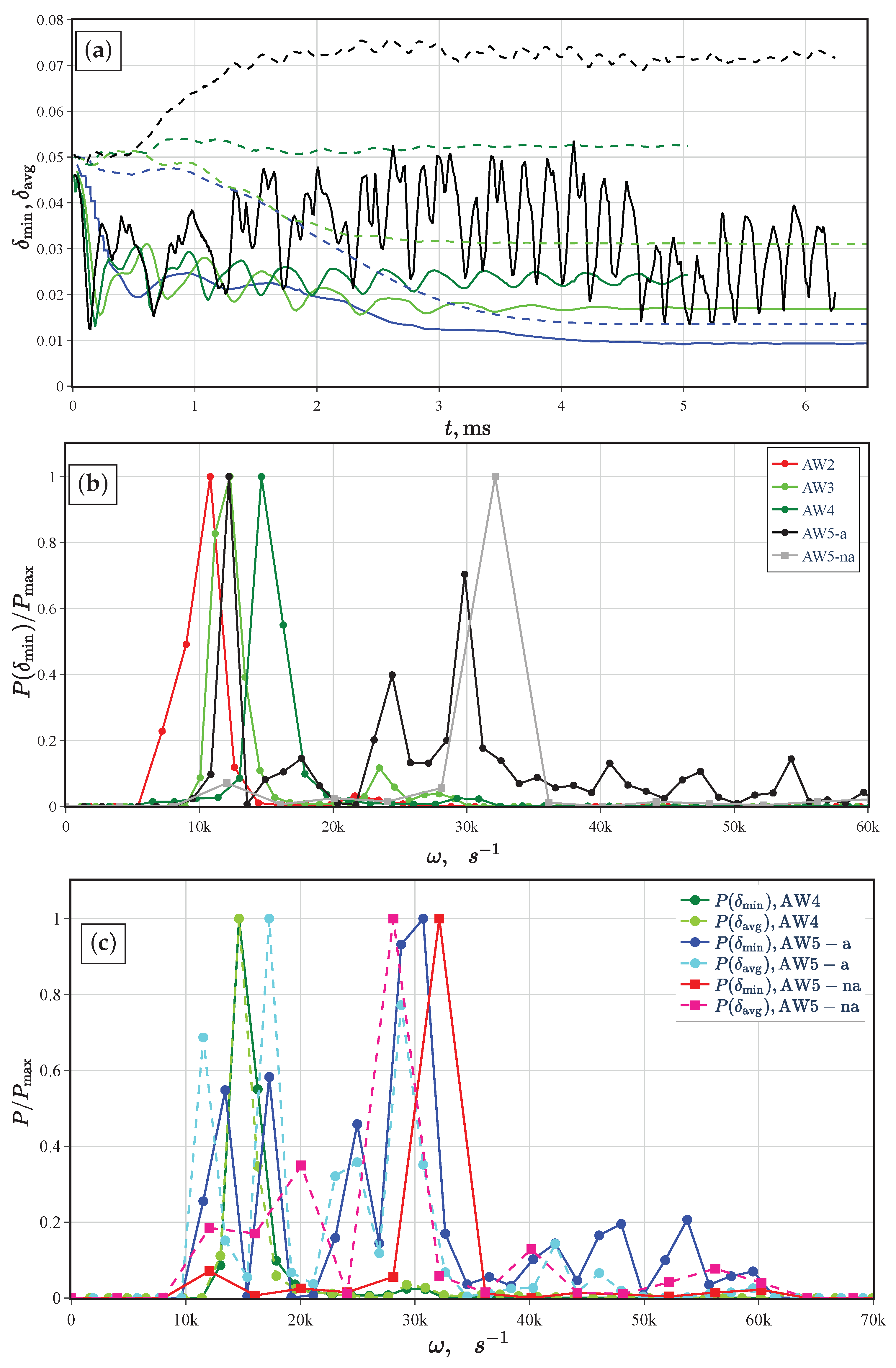

 ), the bubble center of mass ( ), and the tail ( ) relative to the position of the bubble nose for case AW5. (b) The power spectrum of for axisymmetric oscillations at times ms (solid line) and after symmetry breaking at ms (dashed line).
), the bubble center of mass ( ), and the tail ( ) relative to the position of the bubble nose for case AW5. (b) The power spectrum of for axisymmetric oscillations at times ms (solid line) and after symmetry breaking at ms (dashed line).
), the bubble center of mass ( ), and the tail ( ) relative to the position of the bubble nose for case AW5. (b) The power spectrum of for axisymmetric oscillations at times ms (solid line) and after symmetry breaking at ms (dashed line).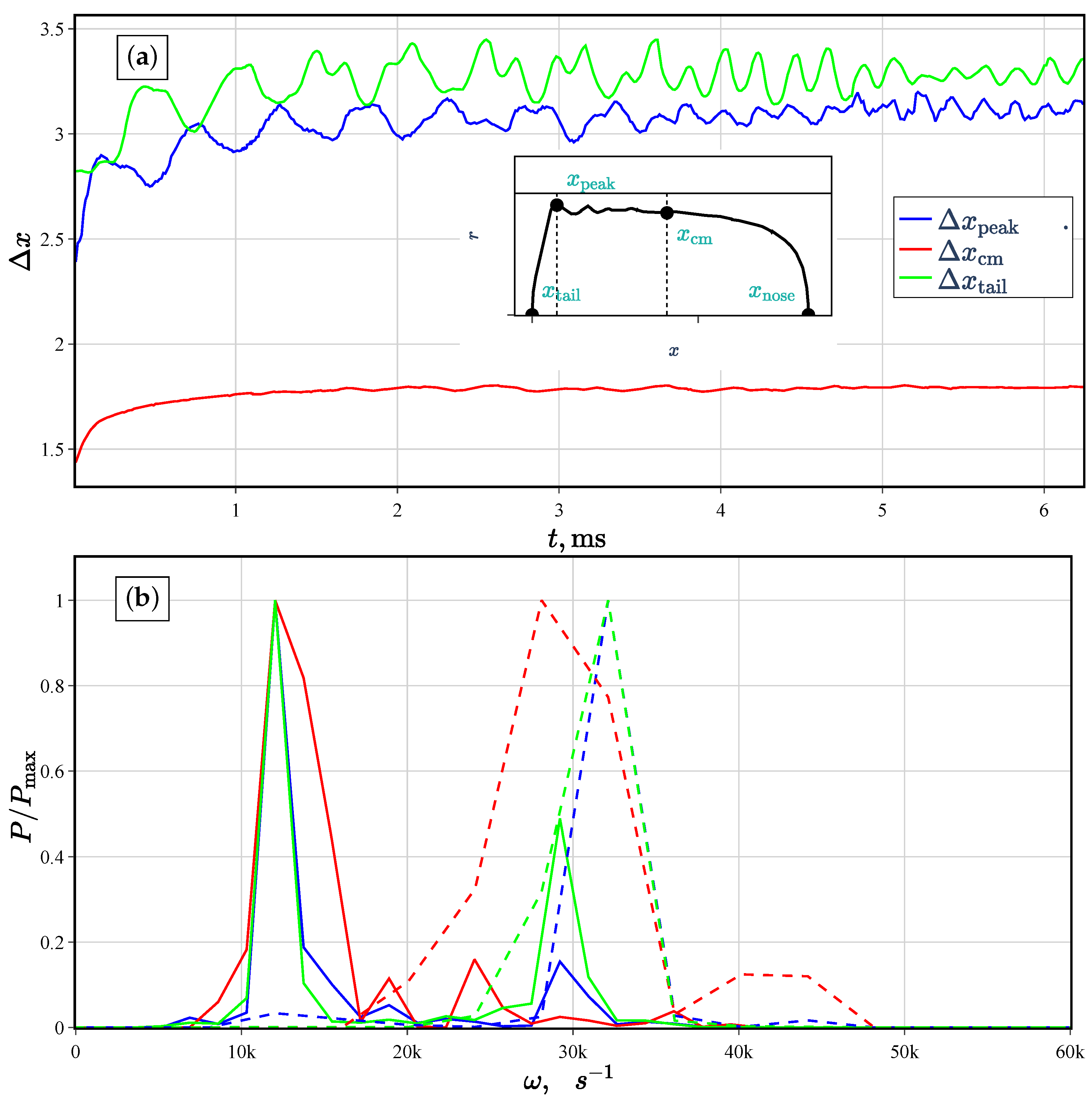

| Names | Ca | Re | l | ||||||||
|---|---|---|---|---|---|---|---|---|---|---|---|
| [23] | BPM | [23] | BPM | ||||||||
| AW1 | 141 | 0.1751 | 0.242 | 20 | 12 | 4 | 0.261 | 0.255 | 0.013 | 0.0173 | |
| AW2 | 388 | 0.1715 | 0.666 | 20 | 12 | 6 | 0.704 | 0.744 | 0.023 | 0.0279 | |
| AW3 | 441 | 0.2208 | 0.757 | 20 | 12 | 7 | 0.815 | 0.854 | 0.025 | 0.031 | |
| AW4 | 651 | 0.1882 | 1.118 | 20 | 12 | 10 | 1.293 | 1.325 | 0.039 | 0.0453 | |
| AW5 | 920 | 0.2179 | 1.580 | 30 | 13 | 20 | 1.944 | 2.005 | 0.054 | 0.0716 | |
| Names | AW1 | AW2 | AW3 | AW4 | AW5-a (Axial) | AW5-na (Not Axial) |
|---|---|---|---|---|---|---|
| — | ||||||
| — |
| Names | Ca | Re | ||||
|---|---|---|---|---|---|---|
| AW5 | 0.024 | 920 | 1.580 | 20 | 2.005 | 0.0716 |
| AW6 | 0.034 | 1200 | 2.060 | 29 | 2.824 | 0.106 |
| AW7 | 0.0455 | 1500 | 2.575 | 20 | 3.76 * | 0.137 * |
| AW8 | 0.056 | 1800 | 3.09 | 20 | 4.65 * | 0.15 * |
Publisher’s Note: MDPI stays neutral with regard to jurisdictional claims in published maps and institutional affiliations. |
© 2021 by the authors. Licensee MDPI, Basel, Switzerland. This article is an open access article distributed under the terms and conditions of the Creative Commons Attribution (CC BY) license (https://creativecommons.org/licenses/by/4.0/).
Share and Cite
Sharaborin, E.L.; Rogozin, O.A.; Kasimov, A.R. Computational Study of the Dynamics of the Taylor Bubble. Fluids 2021, 6, 389. https://doi.org/10.3390/fluids6110389
Sharaborin EL, Rogozin OA, Kasimov AR. Computational Study of the Dynamics of the Taylor Bubble. Fluids. 2021; 6(11):389. https://doi.org/10.3390/fluids6110389
Chicago/Turabian StyleSharaborin, Evgenii L., Oleg A. Rogozin, and Aslan R. Kasimov. 2021. "Computational Study of the Dynamics of the Taylor Bubble" Fluids 6, no. 11: 389. https://doi.org/10.3390/fluids6110389
APA StyleSharaborin, E. L., Rogozin, O. A., & Kasimov, A. R. (2021). Computational Study of the Dynamics of the Taylor Bubble. Fluids, 6(11), 389. https://doi.org/10.3390/fluids6110389