Flagellar Cooperativity and Collective Motion in Sperm

Abstract

Sperm have thin structures known as flagella whose motion must be regulated in order to reach the egg for fertilization. Large numbers of sperm are typically needed in this process and some species have sperm that exhibit collective or aggregate motion when swimming in groups. The purpose of this study is to model planar motion of flagella in groups to explore how collective motion may arise in three-dimensional fluid environments. We use the method of regularized Stokeslets and a three-dimensional preferred curvature model to simulate groups of undulating flagella, where flagellar waveforms are modulated via hydrodynamic coupling with other flagella and surfaces. We find that collective motion of free-swimming flagella is an unstable phenomenon in long-term simulations unless there is an external mechanism to keep flagella near each other. However, there is evidence that collective swimming can result in significant gains in velocity and efficiency. With the addition of an ability for sperm to attach and swim together as a group, velocities and efficiencies can be increased even further, which may indicate why some species have evolved mechanisms that enable collective swimming and cooperative behavior in sperm.

1. Introduction

Many biological cell types rely upon tail-like appendages known as flagella to propel them towards optimal environments or environments where the cell serves a specific function. These flagella must typically move through highly viscous fluids, perhaps in the presence of other objects and cells within the fluid. Collective motion of flagella has long been observed in cells. For example, in bacteria with multiple flagella, flagella can rotate in a helical fashion and form a bundle [1,2]. In mammalian sperm, cells have a single flagellum but flagellar motion may be impacted by neighboring sperm or other structures in the environment.

Sperm motility is a major indicating factor for fertility potential and thus sexual reproduction [3]. Sperm must maneuver through a variety of environments in order to reach the egg and this process involves a complex choreography of biochemical reactions that mediate changes in motility patterns. These motility patterns are undulatory and often characterized by a nearly planar, sinusoidal beat form, though helical or “Figure 8” beat patterns have also been observed [4,5,6,7]. A planar waveform would result in sperm primarily traveling in a planar trajectory, but high resolution 3D trajectories of sperm have shown more intriguing patterns of helical or chiral ribbon trajectories over time [8,9,10,11]. 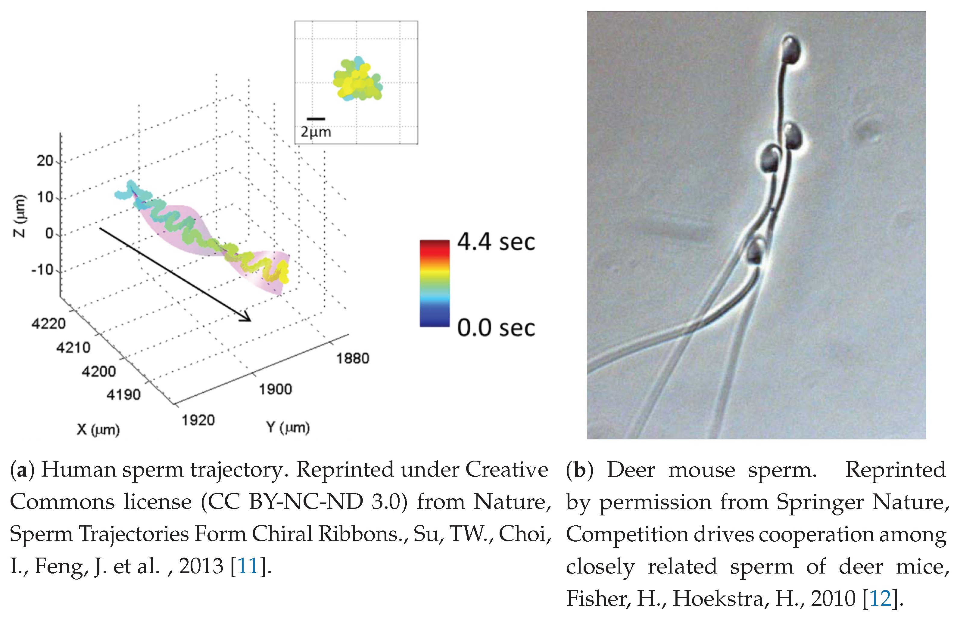Figure 1a shows one example of a chiral ribbon trajectory observed in human sperm.

Species as diverse as deer mouse, cattle, fly, echidna and opossum have sperm that can collectively swim together [12,13,14,15,16,17,18,19]. Figure 1b shows an example of such behavior in the deer mouse, where apical hooks on sperm heads enable sperm to attach to a neighbor’s flagellum. This is sometimes referred to as a sperm train. Swimming with nearby neighbors makes for a highly complex fluid–structure environment in which there is feedback between the fluid and neighboring sperm that will effect velocities and trajectories significantly, and therefore has the potential to impact reproductive success. Moreover, complexity can arise from surface interactions between sperm and the oviductal epithelium, egg or other structures immersed in the fluid. For instance, it is known that sperm will repeatedly bind and unbind to the oviductal epithelium [20,21] and this behavior has an impact on sperm trajectories over time.

Undulating flagella and sperm motility have been the inspiration for mathematical modeling efforts for decades as an ideal system for studying motion in viscous fluids. Models for planar motion of flagella near surfaces includes investigations near a no-slip planar surface [22,23,24,25,26] and a rigid sphere [27]. In general, models have shown that individual sperm tend to be attracted to planar surfaces and stick to them unless the sperm change their waveform (i.e., increase amplitude, asymmetry, or wavenumber) and/or the sperm is kept a small distance away from the planar surface. Near a rigid sphere, sperm may more easily escape the spherical surface though this is dependent on geometry [27].

Mathematical models for flagellar swimming in groups are an active area of research. Some studies have considered 2D fluids, which demonstrated a tendency of flagella to attract and that this attraction is energetically favorable [23,28,29,30]. In 3D fluids, models have shown both attraction and repulsion of neighboring flagellar pairs, but the results are dependent on configurations of the flagella, the fluid domain, timescales of simulation, and the flagellar model. In [29], coplanar swimmers in 3D fluids had increased efficiency. The work of [31] showed gains in velocity for shorter timescale simulations of both coplanar and parallel plane geometries, though results depended on phase. In [32], it was proposed that coplanar attraction was an unstable state, as parallel and nearly coplanar swimmers tended to swim apart, in contrast to attraction seen for perfectly coplanar swimmers. Aggregation of sperm was shown to be a commonly observed behavior in a 2D-periodic thin film in [33]. Interestingly, this aggregation was suppressed with the introduction of stochasticity in the beat frequency. A coarse-grained approach based on experimentally-derived beat patterns showed that sperm clustering is inhibited by low viscosity media and small changes in individual flagellar motion substantially affect clustering dynamics and collective motion [34]. In [35], the authors found evidence for stable pairwise swimming configurations and increases in velocities that may indicate an advantage to cooperative behavior. Moreover, transient attraction of pairs of swimmers and increases in velocities were also demonstrated for coplanar flagella in [36].

Missing in these prior results are broader considerations of three-dimensional geometries of groups of flagellar swimmers with fine-grained models of flagellar motility on long timescales. This is primarily due to the high computational costs of these investigations but also due to restrictions in some modeling assumptions and frameworks. The purpose of this work is to address this gap and provide insight into how swimming in groups and near surfaces affects not only trajectories but also velocities, power expenditures, and efficiency.

The most realistic modeling framework for sperm motility would include a viscoelastic, non-Newtonian fluid model, detailed flagellar waveforms that can be modulated by interactions with other objects, the entire morphology of the sperm head, fully three-dimensional domains and geometries, external fluid flow, and biochemically-mediated interactions between sperm and their environment. At present, putting all of these components together is computationally prohibitive. Thus, prior work has all taken aim at specific pieces of the puzzle. As our interest lies in collective flagellar motion, our priorities are to consider a detailed model of the flagellum that allows for emergent waveforms as in [32,37] instead of prescribed waveforms as in [38], simulate many flagella as done in [33] but with a broader range of geometrical configurations as in [31,32,35], with and without a surface present similar to [25,39] over longer time scales.

Recent work has simulated flagella in pairs for up to 10–20 beats [35] but we will go beyond this here to address any lingering questions about long-range stability of flagellar interactions like those posed in [30]. Simulations involving all of these components are computational expensive due to the finer scale details we aim to resolve but they are plausible, as long as we relax some of other ideal features of a model. In our case, we will focus on purely viscous, Newtonian fluid flow instead of non-Newtonian fluids like those modeled in [30,40]. We will also not consider sperm heads as done in [26], external fluid flow such as [41], or more detailed biochemical interactions like those described in [37,42]. These choices not only keep our simulations tractable, but also allow for direct comparison with prior, related work including [32,43].

As a first approximation, we will be using a planar flagellar motility model that is capable of bending in three dimensions when a flagellum is pushed out of its native plane. This model was developed in [32] and is based on prior work developed in [37,44]. Here, we extend this work to consider groups of more than two flagella and add a new component to the model to allow neighboring flagella to attach along each other’s length to mimic apical hooks. This model is related to the work in [33], but we do not consider a thin-film (a nearly 2D setting) nor do we include periodicity in our fluid environment. Therefore, the environments we are modeling are less spatially constrained and less dense than in [33], but provide the ability to analyze a broad range of 3D configurations and yet still focus on individual interactions between swimmers. In comparison to [34], our flagellar motility model is not coarse grained, allows for changes in the beat pattern when flagella encounter other objects within the fluid, and allows for a more detailed analysis of individual flagellar behaviors.

In this paper, we will consider groups of flagella up to 9, in a variety of configurations, both with and without surfaces present. We employ the method of regularized Stokeslets [45] due to the need for computational solutions to solve the governing equations of viscous fluid environments. In this modeling framework, planar surface dynamics have been studied but only in more restrictive geometries for individual swimmers in [25]. Therefore, this present work is a new exploration of surface dynamics for groups of flagellar swimmers, with no spatial restrictions for flagellar configurations. In this way, we will be able to explore the importance of swimming in groups in viscous environments and interpret the behavior of populations of sperm observed in 3D experimental imaging in [8,9,10,11] as well as the observed cooperative behavior we see in species discussed in [12,13,14,15,16,17].

2. Materials and Methods

The modeling framework we use is a simple extension of the work in [32,46]. We detail the components of the model below.

2.1. Fluid Model

Flagellar motility in realistic biological settings is characterized by highly viscoelastic, non-Newtonian fluid environments. In laboratory settings, fluid environments can be varied between viscous and viscoelastic regimes, both with low Reynolds numbers. For average mammalian sperm dimensions, the Reynolds number is on the order of ${10}^{-2}$ (see Table 1). Recent work has highlighted that assuming a zero Reynolds number may not always be appropriate for modeling the motion of cilia and flagella [47], but here we will assume a Newtonian fluid with zero Reynolds number for simplicity and to facilitate comparisons with prior work involving similar models. Thus, we model the fluid environment in 3D using the incompressible Stokes equations below:

$$\begin{array}{cc}\hfill \mu \Delta \mathbf{u}& =\nabla p-\mathbf{F}(\mathbf{x},t)\hfill \\ \hfill \nabla ·\mathbf{u}& =0.\hfill \end{array}$$

(1)

In these equations, $\mu$ is the dynamic viscosity, $\mathbf{u}$ is the fluid velocity, p is pressure, $\mathbf{F}$ is the force density and $\mathbf{x}$ and t are the spatial and temporal coordinates, respectively.

The flagella in our simulations exert forces along their length and therefore, we use the following formulation for $\mathbf{F}$:

$$\mathbf{F}(\mathbf{x},t)=\sum _m{\int }_0^L\mathbf{f}({\mathbf{X}}_m(s,t),t){\varphi }_{ϵ}\left(\right||\mathbf{x}-{\mathbf{X}}_m(s,t)\left|\right|)ds.$$

(2)

The integral term represents all forces that are exerted by the $m^{th}$ flagellum. L is the flagellum length, s is the arc length along the flagellum, and ${\mathbf{X}}_m(s,t)$ is the spatial position along the length of the $m^{th}$ flagellum. The function ${\varphi }_{ϵ}\left(r\right)$ is an approximation to the Dirac delta function, often referred to as a blob function or regularized delta function. There are many choices for blob functions, but here we will employ one that has been used in previous studies related to this work [32,43]:

$${\varphi }_{ϵ}\left(r\right)=\frac{15{ϵ}^4}{8\pi {(r^2+{ϵ}^2)}^{7/2}}.$$

(3)

In simulations with a surface included, we require additional terms to enforce a no-slip boundary condition at the surface. We use the method of images to accomplish this, as derived in [46].

2.2. Flagellum Model

The flagella in our model will all be identical, with the exception of their spatial positions and beat planes. Each flagellum is considered a three-dimensional curve in space with forces exerted along the curve. In order to conceptualize these forces, we define a local frame of reference for each flagellum m as follows: translate the flagellum position ${\mathbf{X}}_m(s,t)$ so its center of mass is at the origin, and rotate the flagellum so its beat plane is $z=0$. We will refer to flagellar coordinates in the local frame of reference as ${\widehat{\mathbf{X}}}_m(s,t)$.

The forces that govern the motion of the flagella include tensile forces that keep the curve connected and roughly inextensible, bending forces that actuate the motion of the curve, and planar restriction forces that keep the curve in a nearly planar configuration. Each of these forces is derived from the following continuous energy formulations:

$$\begin{array}{cc}\hfill {\mathcal{E}}_{tens}({\widehat{\mathbf{X}}}_m,t)& =\frac{1}{2}{S}_t{\int }_0^L{\left[∥\frac{\partial {\widehat{\mathbf{X}}}_m}{\partial s}∥-1\right]}^{2}ds\hfill \end{array}$$

(4)

$$\begin{array}{cc}\hfill {\mathcal{E}}_{bend}({\widehat{\mathbf{X}}}_m,t)& =\frac{1}{2}{S}_b{\int }_0^{\ell }{\left[\left(\frac{\partial {\widehat{\mathbf{X}}}_m}{\partial \alpha }\times \frac{{\partial }^2{\widehat{\mathbf{X}}}_m}{\partial {\alpha }^2}\right)·{\mathbf{e}}_3-C_m(\alpha ,t)\right]}^{2}d\alpha \hfill \end{array}$$

(5)

$$\begin{array}{cc}\hfill {\mathcal{E}}_{plane}({\widehat{\mathbf{X}}}_m,t)& =\frac{1}{2}{S}_p{\int }_0^L{\left[\frac{\partial {\widehat{\mathbf{X}}}_m}{\partial s}·{\mathbf{e}}_3\right]}^{2}ds.\hfill \end{array}$$

(6)

Equation (4) is the continuous version of a tensile energy of an ideal spring model. Equation (5) is a bending energy that actuates the flagellum to move towards the planar preferred curvature given by $C_m(\alpha ,t)$, which is chosen to mimic sinusoidal flagellar undulation by setting

$$C_m(\alpha ,t)={\kappa }^{2}bsin(\kappa \alpha -\omega t).$$

(7)

The parameter $\alpha$ is used instead of s here, because while the flagellum can be in a three-dimensional configuration, the beating behavior is planar and therefore $\alpha$ is the projection of the true arc length s onto the flagellar beat plane. Similarly, ℓ represents the full arc length of the flagellum after projection onto the beat plane. Equation (6) is the planar restriction energy, which is an energy that measures local deviations out of the beat plane. The vector ${\mathbf{e}}_3={[0,0,1]}^T$ is the normal vector to the beat plane in the local frame of reference. All $S_i$ values are stiffness parameters. In particular, $S_t$ is chosen to be relatively stiff to enforce inextensibility of the flagellum. For further details, see [44] for the derivation of Equations (4) and (5) and [32] for further explanation of Equation (6).

In the local frame of reference, forces exerted along the flagellum length are then given by:

$$\widehat{\mathbf{f}}({\widehat{\mathbf{X}}}_m,t)=-\frac{\partial \mathcal{E}}{\partial {\widehat{\mathbf{X}}}_m}$$

(8)

where $\mathcal{E}={\mathcal{E}}_{tens}+{\mathcal{E}}_{bend}+{\mathcal{E}}_{plane}$. The forces $\mathbf{f}({\mathbf{X}}_m,t)$ are then found by rotating and translating $\widehat{\mathbf{f}}({\widehat{\mathbf{X}}}_m,t)$ back into the original frame of reference for ${\mathbf{X}}_m$. Such forces move the flagellum towards a minimal energy configuration.

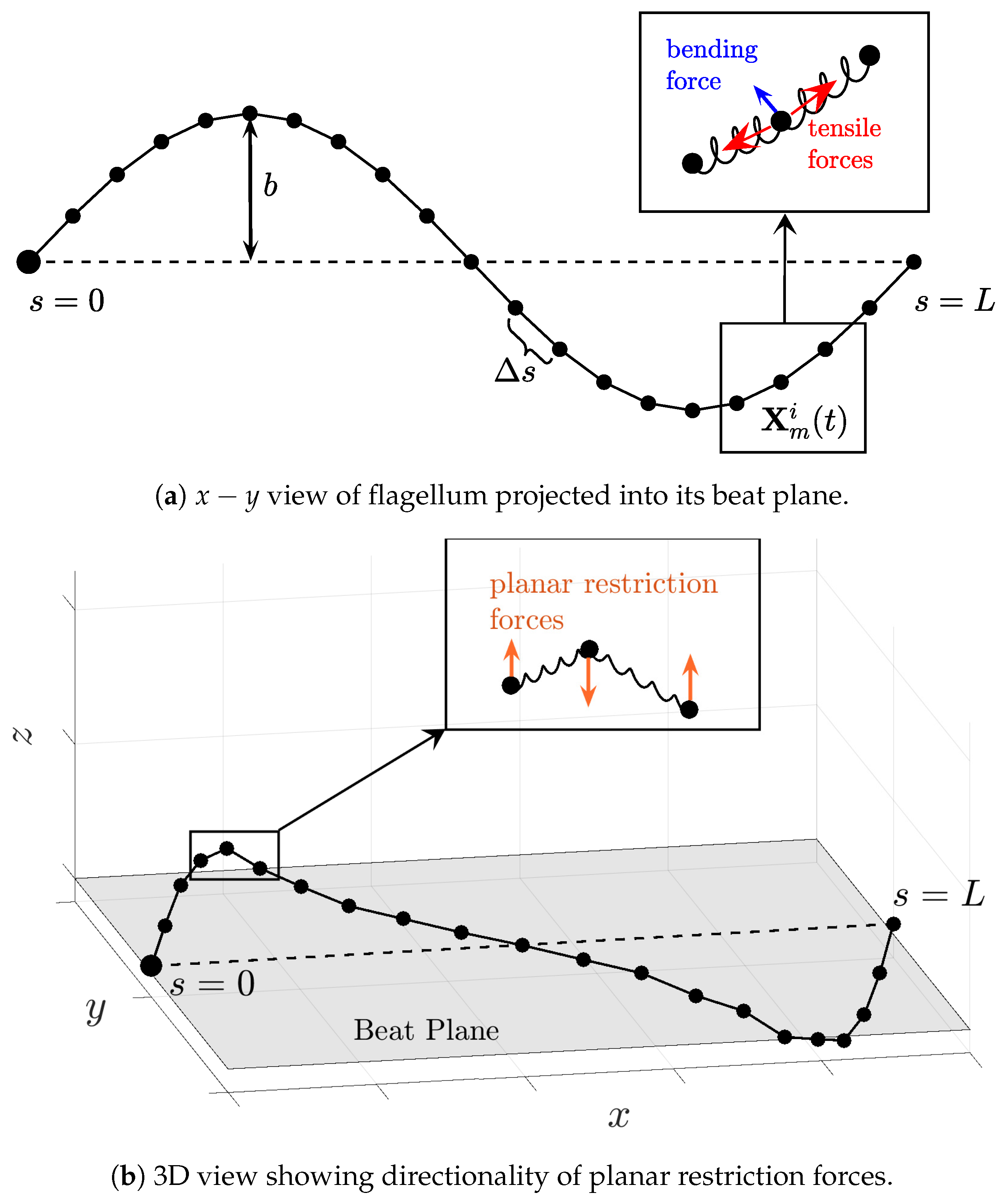
Because we will be simulating flagellar motion computationally, we discretize the spatial coordinates ${\mathbf{X}}_m$ and the forces $\mathbf{f}({\mathbf{X}}_m,t)$ by evenly distributing points along the flagellum as depicted in Figure 2. Thus, we will be modeling the motion of each point ${\mathbf{X}}_m^i$ (the $i^{th}$ point along the $m^{th}$ flagellum) that arises from discretized forces denoted by ${\mathbf{f}}_m^i$, which are derived from discretizing the energies in Equations (4)–(6) along each flagellum. Figure 2 is a schematic representing the forces derived from Equations (4)–(8) and what they mean in the 2D beat plane, as well as the forces out of the beat plane, resulting from Equation (6) specifically.

As done in [32], we add an additional repulsive force to each ${\mathbf{f}}_m^i$ to prevent flagella from unrealistically passing through each other. We denote this repulsion force by ${\mathbf{g}}_m^i$ and define it as:

$${\mathbf{g}}_m^i=\sum _n\sum _j{S}_r\left(\frac{1}{d_r}-\frac{1}{min(r_n^j,d_r)}\right)({\mathbf{X}}_m^i-{\mathbf{X}}_n^j)$$

(9)

where $r_n^j$ is given by $r_n^j=∥{\mathbf{X}}_m^i-{\mathbf{X}}_n^j∥$ and $d_r$ is a small threshold distance in which the repulsion force is added. This effectively keeps individual points (denoted by i and j) along neighboring flagella (denoted by m and n, respectively) from overlapping.

This model for flagellar motion allows for waveforms to emerge and be modulated by their external environment. Such modulations would occur when flagella are close enough to surfaces and other flagella. This flagellar model is computationally expensive when compared to coarse-grained flagellar models (such as [34]) or prescribed motion models such as [31,39], but necessary so we can pursue a more detailed analysis of flagellar cooperativity and surface interactions.

2.3. Coupling the Flagella and Fluid Environment

Forces that the flagella exert in our fluid will move the fluid in accordance with the incompressible Stokes Equation (1). If each force were modeled as a point force, the solution to the fluid velocity field could be found using a summation of Stokeslets (the fundamental solution to the incompressible Stokes Equation (1)), due to the linearity of these equations. As we aim to simulate flagellar motion computationally, we use the blob function given in Equation (3) and therefore solutions will be a summation of regularized Stokelets, which are solutions to the incompressible Stokes Equations derived from the blob function [45]. In our case, the fluid velocity in free space is:

$${\displaystyle \mathbf{u}\left(\mathbf{x}\right)=\sum _m\sum _i\frac{r_{i,m}^2+2{ϵ}^2}{{(r_{i,m}^2+{ϵ}^2)}^{3/2}}{\mathbf{f}}_m^i+\frac{\left({\mathbf{f}}_m^i·(\mathbf{x}-{\mathbf{X}}_m^i)\right)(\mathbf{x}-{\mathbf{X}}_m^i)}{{(r_{i,m}^2+{ϵ}^2)}^{3/2}}}$$

(10)

where $r_{i,m}=∥\mathbf{x}-{\mathbf{X}}_m^i∥$ and $ϵ$ is a small parameter. This is a summation of regularized Stokeslets over all m flagella and all i points along each flagellum.

2.4. Model for Apical Hooks

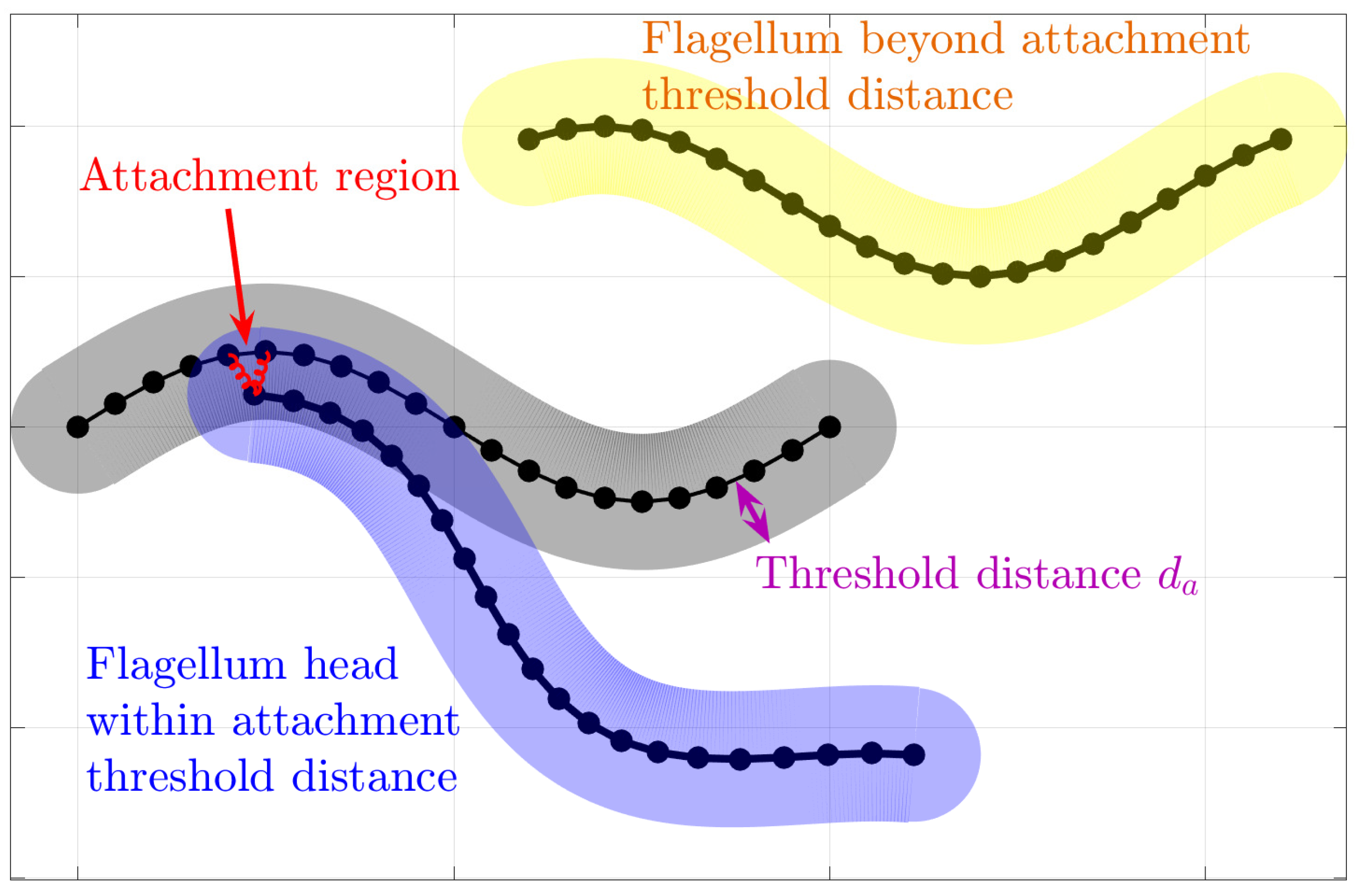
In an attempt to understand the collective motion of sperm that have been observed to attach to each other, we choose to focus on the sperm train behavior shown in Figure 1b, which has been observed in deer mice as [12]. These so-called trains arise, at least in part, due to an apical hook on the sperm head that allows a sperm to attach to the flagellum of another sperm. Instead of modeling the morphology of the hook that can attach to neighboring flagella, we simply add forces at the head (initial point) of flagellum m and along the neighboring flagellum n if the head of flagellum m gets within a threshold distance, $d_a$, of the neighboring flagellum n.

The forces added are a simple spring force model that effectively holds the head of the flagellum close to the neighboring flagellum points, with a fixed resting length a. The mathematical formulation to model for this attachment behavior can be expressed as:

$${\mathbf{h}}_{m,n}^j=\left\{\begin{array}{cc}{S}_a\left(∥{\mathbf{X}}_n^j-{\mathbf{X}}_m^1∥-a\right)\frac{{\mathbf{X}}_n^j-{\mathbf{X}}_m^1}{∥{\mathbf{X}}_n^j-{\mathbf{X}}_m^1∥}\hfill & \mathrm{if}∥{\mathbf{X}}_n^j-{\mathbf{X}}_m^1∥<d_a\hfill \\ 0\hfill & \mathrm{otherwise}\hfill \end{array}\right.$$

(11)

Note that this force is applied at the head (first point) of the flagellum m but also in equal magnitude but opposite direction at nearby points j along the neighboring flagellum n, so both flagella will be impacted by the attachment. Figure 3 shows a schematic of the attachment model.

This is not a permanent bond between the flagella, but rather forces that persist as long as the head of one flagellum remains close enough to another flagellum. This attachment does not prevent rotation of the flagella, or translational movement of the flagella along each other. These details are important as a hook around a flagellum might allow for some motion up and down the flagellum, and would not necessarily prevent rotation around the hook attachment region.

We note that the model described in Equation (11) is similar to models used in other investigations involving cell adhesion. For instance, a similar spring-like adhesion force to model receptor-ligand binding between particles and walls in the context of blood flow has been used for many years [48,49,50,51]. Our model differs in four main ways from such work. First, these works are considering whole cells with distributions of many nano-structures (receptors) on their surface that can bind to ligands on epithelial surfaces. Our model has no surface of a cell, but rather a single point at the head of the flagellum that can bind. Second, bond formation and dissolution is different: for our model, the apical hook force is applied only when flagellar heads are within a fixed distance of another flagellum, whereas there is a probabilistic approach for forming and breaking bonds in [48,49,50,51]. Third, we are modeling a much larger structure than receptors and ligands. An apical hook is a macrostructure of the sperm head and would not necessarily experience the same types of probabilistic effects of forming and breaking bonds that we see in receptor-ligand dynamics. Lastly, our apical hook model enables binding between one flagellum and another flagellum, which are both freely moving curves in space, rather than a cell body and a surface.

2.5. Computational Method

Our computational method is as follows:

• Initialize flagella in desired configuration.
• Every time step:

  (a)

  Compute forces on all flagella, including tensile, bending, and planar restriction forces. If applicable, compute attachment or repulsion forces.

  (b)

  Find the velocity at each point along flagella using regularized Stokeslets.

  (c)

  Move flagellar points ${\mathbf{X}}_m^i$ according to velocity at that point, $\mathbf{u}\left({\mathbf{X}}_m^i\left(t\right)\right)$, using a forward Euler method with time step $\Delta t$.

2.6. Parameters and Initial Configurations of Flagella

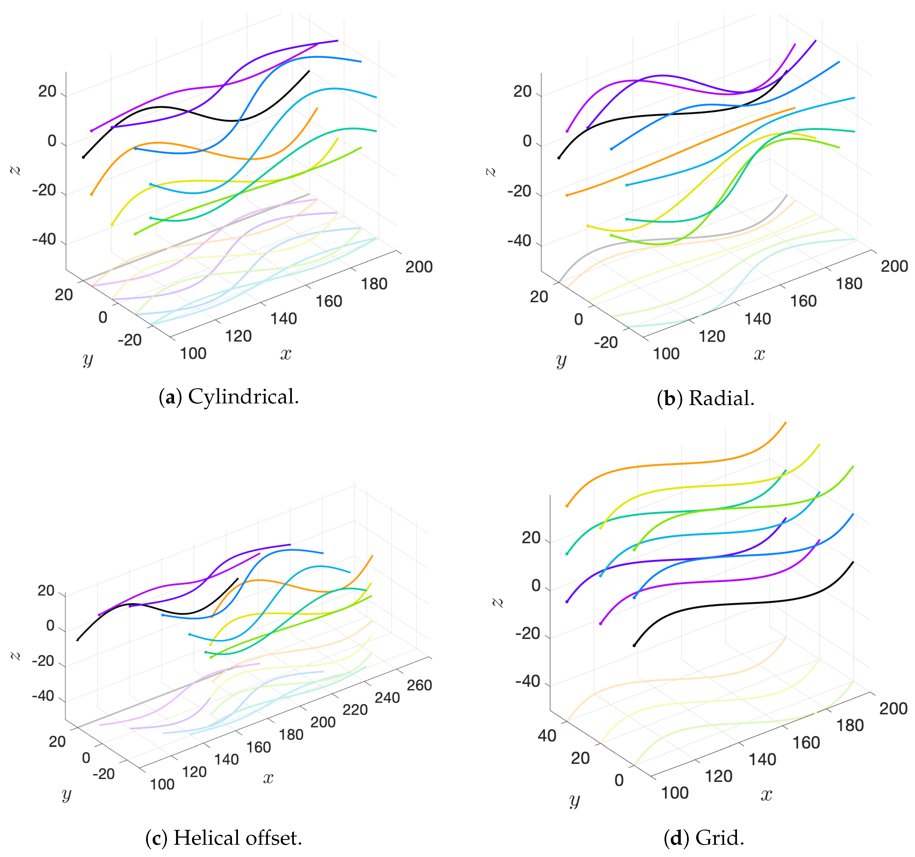
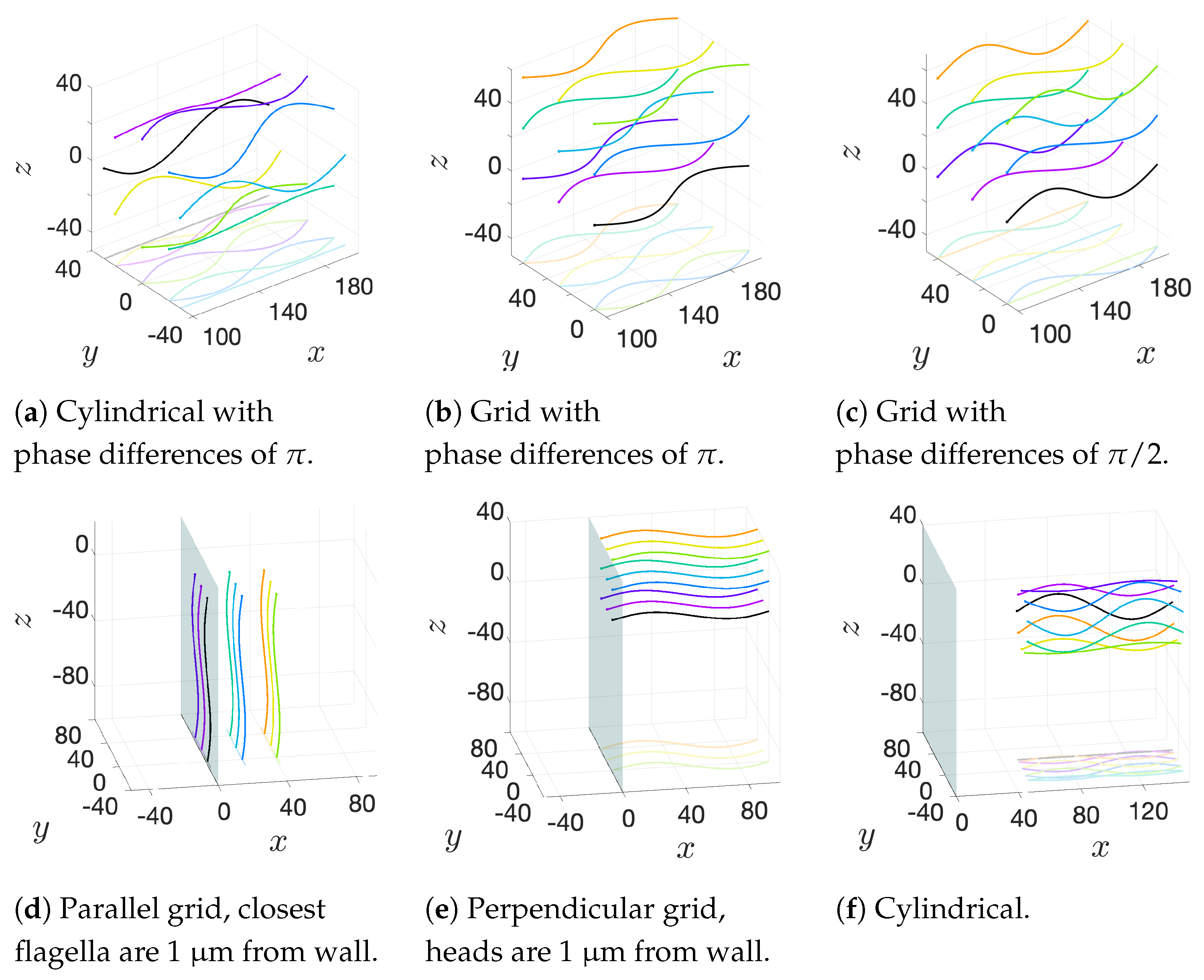
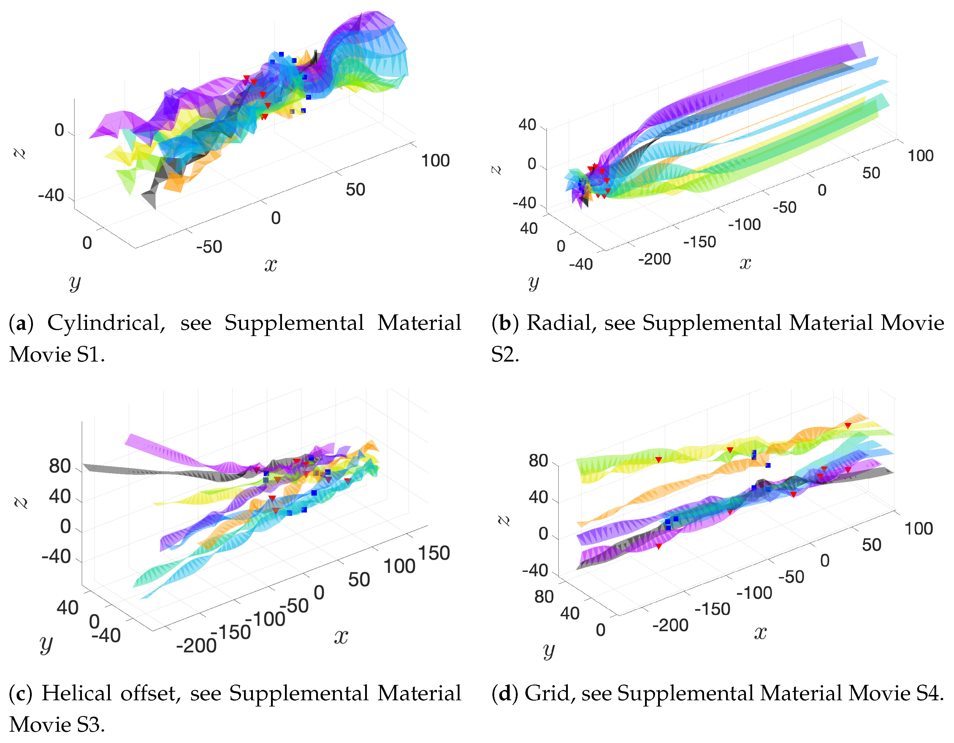
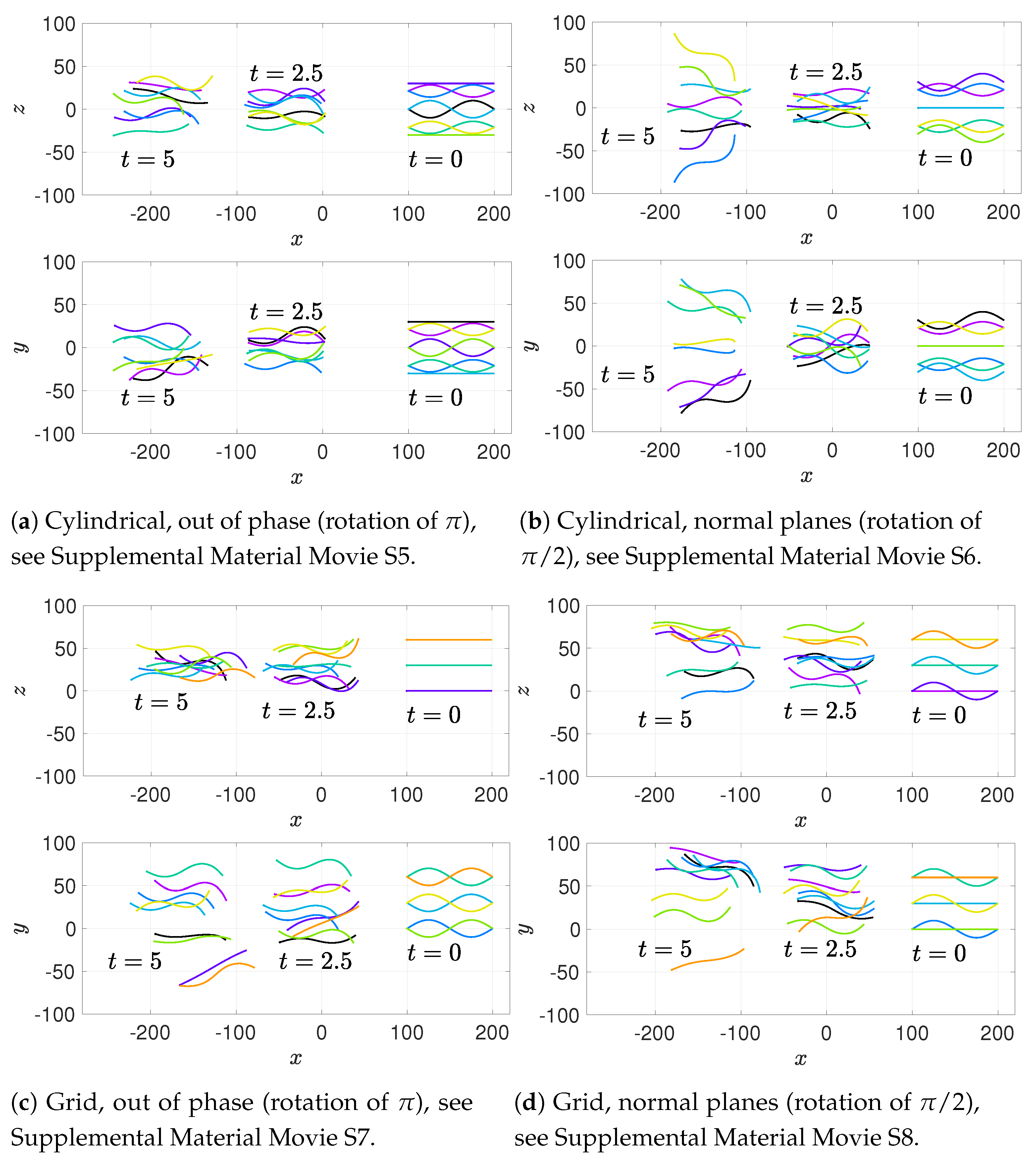
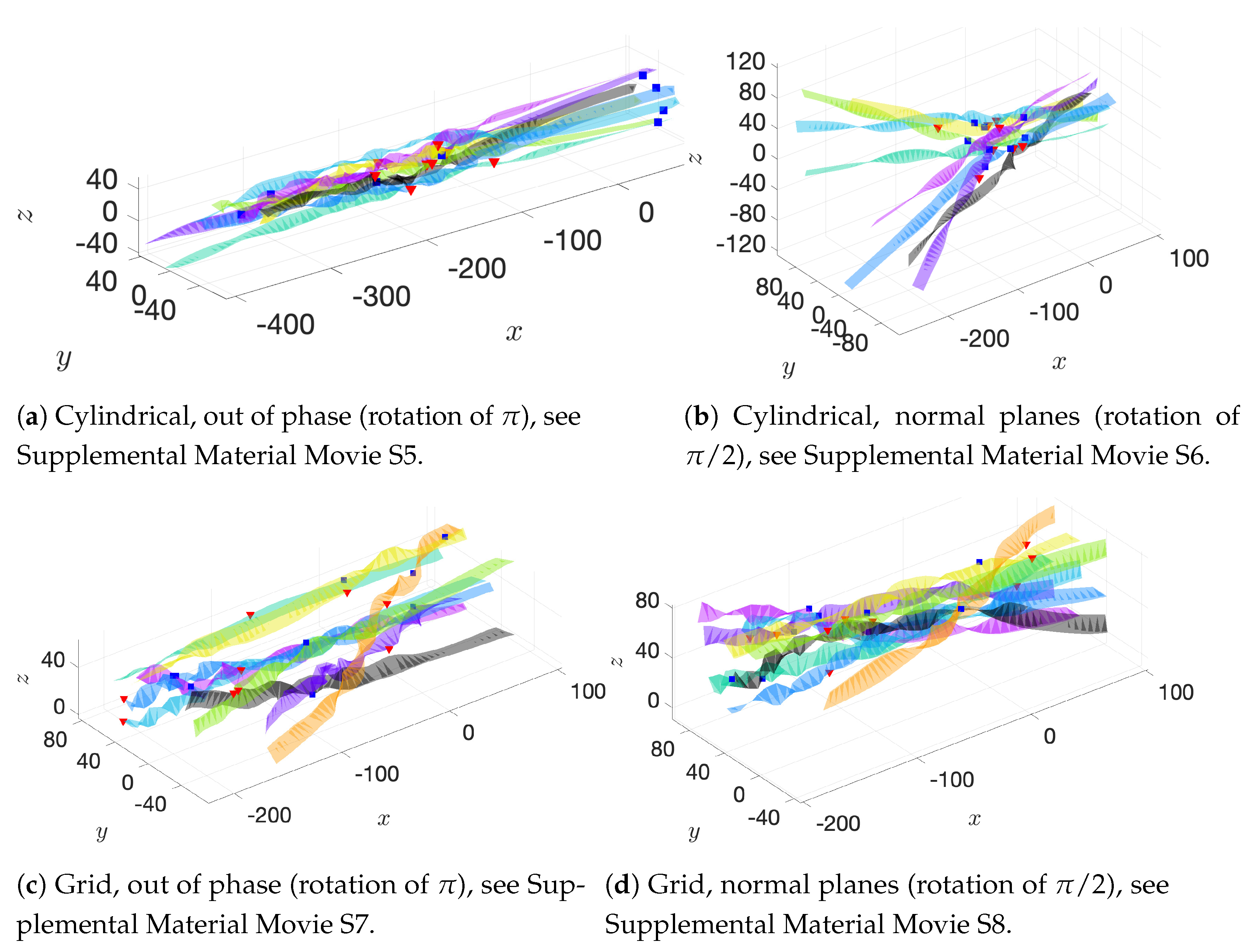
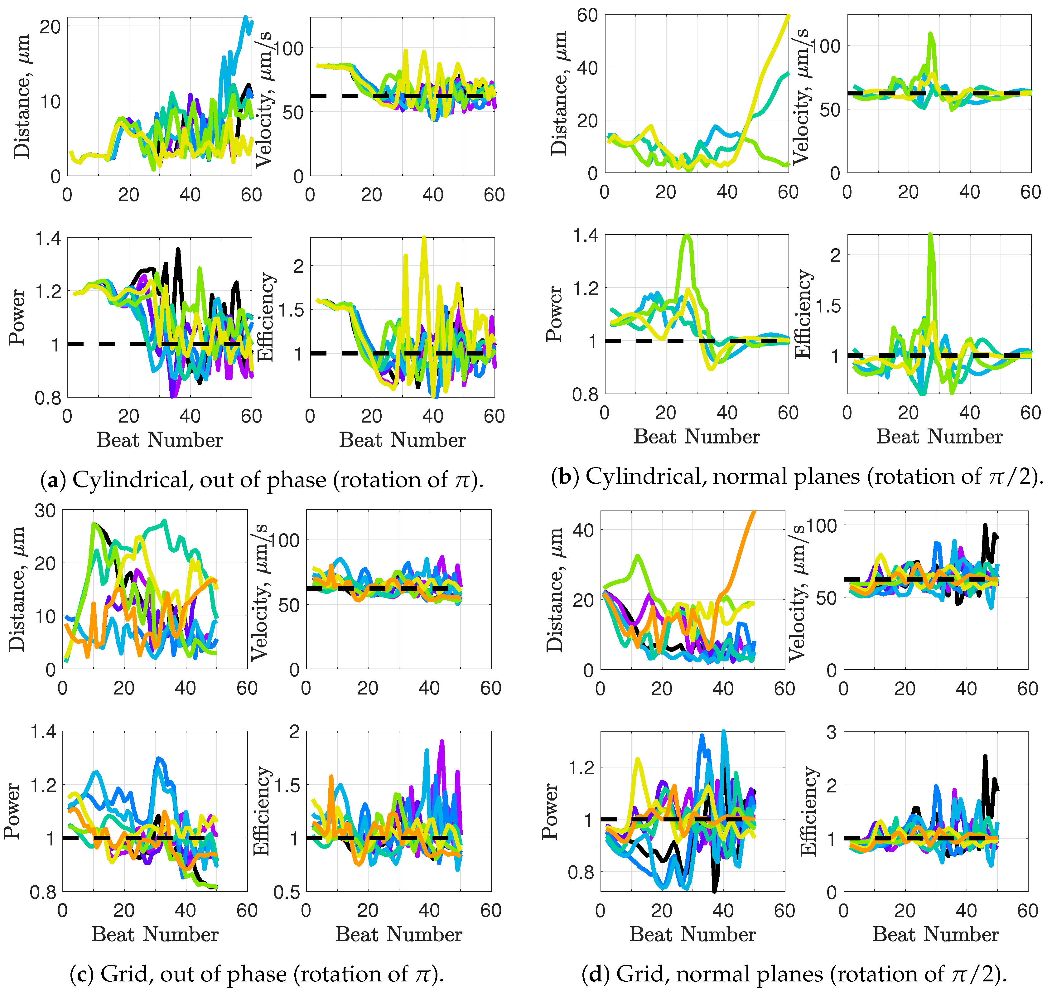
We will consider a variety of initial configurations of flagella, which are based on geometries that allow for an exploration of symmetry and phase. While there are infinitely many configurations that we could consider, we restrict ourselves to the following scenarios in order to exploit symmetry and compare and contrast effectively:

• Cylindrical: flagellar planes tangent to a cylinder;
• Radial: flagellar planes normal to a cylinder;
• Helical offset: cylindrical pattern of neighboring flagella set back along a cylindrical surface to form a helical shape; and
• Grid: all flagella are aligned with bodies in grid patterns.

These basic initial configurations are shown in Figure 4 for groups of 9 swimmers.

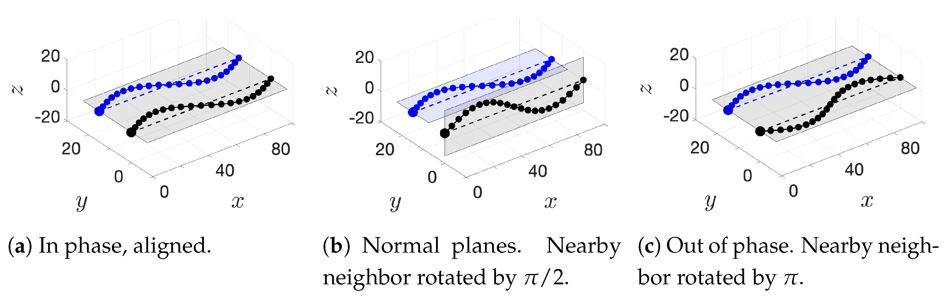
In addition to these basic initial configurations, we also wish to consider phase or alignment differences between flagella. To do so, we rotate nearest neighboring flagella along their centerline axis by one of two angles:

• $\pi /2$: we will refer to this as a “normal plane” configuration. Neighboring flagella have beat planes that are normal or nearly normal to each other. Motion of neighboring flagella are neither in phase (aligned) nor in opposition.
• $\pi$: we will refer to this rotation as an “out of phase” configuration. Neighboring flagella will be completely out of phase or nearly out of phase, but with similar beat planes. Similar here means identical, parallel, or nearly parallel beat planes. Motions of neighboring flagella are generally expected to push and pull in opposition to each other.

While we are not changing the phase of flagella explicitly, the rotations do enable some exploration of the role of phase. See Figure 5 for a graphical representation of these rotations.

Figure 6a–c show depictions of how we combine the alignment schemes of Figure 5 with the basic initial configurations introduced in Figure 4. Figure 6d–f show the initial configurations we will use when considering a planar surface (or wall) nearby. Lastly, all parameter values are listed in Table 1.

Table 1. Parameter values. Sperm parameters were set to that of a typical mammalian sperm with active motility. Wherever possible, biologically-measured values were used. In absence of biologically-measured values, values from prior modeling work were used, if they exist.

Parameter	Parameter	Parameter	Remark/Reference(s)
$ϵ$	Regularization parameter	1.3 $\mathsf{\mu }$m	[45]
	Diameter of sperm flagellum	0.5 $\mathsf{\mu }$m	[52]
$\mu$	Viscosity (water)	10${}^{-3}$ kg m${}^{-1}$ s${}^{-1}$
$\Delta s$	Spatial (arc length) discretization	1 $\mathsf{\mu }$m	Set to be $<ϵ$ [25,32]
L	Flagellum length	100 $\mathsf{\mu }$m	[53]
b	Amplitude	10 $\mathsf{\mu }$m	[54,55]
$\kappa$	Wavenumber	$2\pi /L$	[5]
$\omega$	Frequency	20$\pi$ (10 Hz)	[54,55]
$S_t$	Tensile stiffness	2 pN $\mathsf{\mu }$m${}^{-3}$	[25,32]
$S_p$	Planar restriction stiffness	1 pN $\mathsf{\mu }$m${}^{-3}$	[32]
$S_b$	Planar bending stiffness	10 pN $\mathsf{\mu }$m${}^{-3}$	[37]
$S_r$	Repulsion stiffness	5 aN $\mathsf{\mu }$m${}^{-3}$	[32]
$S_a$	Attachment stiffness	20 fN $\mathsf{\mu }$m${}^{-3}$	Set to be $<S_t$, this work
$d_r$	Repulsion length	3 $\mathsf{\mu }$m	Set to be $>2ϵ$ [32]
$d_a$	Attraction threshold	10 $\mathsf{\mu }$m	This work
a	Attachment length	6 $\mathsf{\mu }$m	Close to sperm head dimensions [53]
V	Average path velocity	$\approx {10}^{-5}$–${10}^{-4}$ m/s	[56]
$\rho$	Density (water)	${10}^3$ kg m${}^{-3}$
$Re$	Reynolds number	$\approx {10}^{-2}$

Table 1. Parameter values. Sperm parameters were set to that of a typical mammalian sperm with active motility. Wherever possible, biologically-measured values were used. In absence of biologically-measured values, values from prior modeling work were used, if they exist.

Parameter	Parameter	Parameter	Remark/Reference(s)
$ϵ$	Regularization parameter	1.3 $\mathsf{\mu }$m	[45]
	Diameter of sperm flagellum	0.5 $\mathsf{\mu }$m	[52]
$\mu$	Viscosity (water)	10${}^{-3}$ kg m${}^{-1}$ s${}^{-1}$
$\Delta s$	Spatial (arc length) discretization	1 $\mathsf{\mu }$m	Set to be $<ϵ$ [25,32]
L	Flagellum length	100 $\mathsf{\mu }$m	[53]
b	Amplitude	10 $\mathsf{\mu }$m	[54,55]
$\kappa$	Wavenumber	$2\pi /L$	[5]
$\omega$	Frequency	20$\pi$ (10 Hz)	[54,55]
$S_t$	Tensile stiffness	2 pN $\mathsf{\mu }$m${}^{-3}$	[25,32]
$S_p$	Planar restriction stiffness	1 pN $\mathsf{\mu }$m${}^{-3}$	[32]
$S_b$	Planar bending stiffness	10 pN $\mathsf{\mu }$m${}^{-3}$	[37]
$S_r$	Repulsion stiffness	5 aN $\mathsf{\mu }$m${}^{-3}$	[32]
$S_a$	Attachment stiffness	20 fN $\mathsf{\mu }$m${}^{-3}$	Set to be $<S_t$, this work
$d_r$	Repulsion length	3 $\mathsf{\mu }$m	Set to be $>2ϵ$ [32]
$d_a$	Attraction threshold	10 $\mathsf{\mu }$m	This work
a	Attachment length	6 $\mathsf{\mu }$m	Close to sperm head dimensions [53]
V	Average path velocity	$\approx {10}^{-5}$–${10}^{-4}$ m/s	[56]
$\rho$	Density (water)	${10}^3$ kg m${}^{-3}$
$Re$	Reynolds number	$\approx {10}^{-2}$

3. Results

Each simulation was run for many beats (on the order of 50–100) in order to observe motility patterns that arise in populations over long timescales. Movies showing results from all simulations are provided in the Supplemental Materials. In addition to spatial swimming patterns, we computed the average velocity, power, and efficiency per beat as well as the minimal distance between each flagellum and all of its neighbors. Our goal is to understand efficiency and behavior of populations of flagella compared to a single flagellum in free space, so we report all quantitative metrics in reference to a single swimmer in free space.

The average velocity V is an average path velocity magnitude, computed over one beat. Power exerted at time t is defined as:

$$P_m\left(t\right)={\int }_{s=0}^L\mathbf{u}({\mathbf{X}}_m(s,t),t)·\mathbf{f}({\mathbf{X}}_m(s,t),t)ds.$$

(12)

We discretize this formulation, since our velocities and forces are discrete, using the trapezoidal rule, as in [43]. For a single flagellum, we expect power to oscillate over the period of a beat, so we use the total power per beat, ${\overline{P}}_m$, as a metric to understand typical power expenditures for each flagellum:

$${\overline{P}}_m=\frac{\omega }{2\pi }\sum _{n=0}^{N_b}{P}_m(n\Delta t)\Delta t.$$

(13)

where $\Delta t$ is the time discretization, n is the time step, $N_b$ is the number of time steps per beat, and $\omega$ is the beat frequency. Finally, we use the following metric for efficiency per beat:

$$\beta =\frac{V^2}{{\overline{P}}_m}.$$

(14)

This definition of efficiency is often used for efficiency measures and was also used in [43].

3.1. In Phase Simulations

For all configurations shown in Figure 4, we initialized the flagella in phase with respect to their nearest neighbors. In a cylindrical or radial configuration, this means that flagellar beating patterns are aligned (i.e., in phase) but with rotation of the beat plane and translation of flagellar bodies to create a circular pattern. The results of all simulations are shown in Figure 7, Figure 8, Figure 9, Figure 10 and Figure 11 and in Movies S1–S4 provided in the Supplemental Materials.

Figure 7 shows 2D snapshots of flagellar positions over time, overlaid, in which we see both attraction of flagella and divergence of flagella. Each set of flagella is shown 2.5 s apart, or 25 beats apart. Thus, you can see differences not only in behavior but also in how far the flagella have traveled over time (an indicator of velocity). Note that the slowest swimmers are those in the cylindrical configuration.

This can be further understood by looking at the trajectories of each flagellum over time. There are different ways to visualize this. For instance, if we want to view the average path of the flagellum over time, we can plot the location of the sperm head once per beat (to remove the lateral oscillation of the head within the beat). We show two examples of this approach in Figure 8 for the cylindrical and radial simulations. Notice that in both of these simulations, the average path trajectories attract towards each other for a transient period of time before the paths ultimately diverge. For instance, in Figure 8a, we see flagella are attracting in the initial part of the configuration. This is highlighted with the inset showing the y-z plane of the trajectories for the first 1.4 s or 14 beats. In contrast, the initial radial configuration in Figure 8b shows slight divergence of flagella initially with a subsequent attraction phase followed by divergence near the very end.

The behavior in Figure 8 is also shown in Movies S1 and S2 given in the Supplemental Material. These movies indicate that flagella in a more cylindrical configuration will have a “steering wheel”-like behavior as the group of flagella undulate in a circular fashion. This action can become quite pronounced as the flagellar heads approach one another, though this is a transient behavior.

Another was to visualize flagellar trajectories is to also include the lateral head displacement throughout the beat. This will carve out a zig-zag path that can be triangulated to show a ribbon-like path. These ribbons indicate the beat plane, which will provide a sense for how flagellar bodies are rotating. The ribbon path trajectories for all in phase simulations are shown in Figure 9. The twisting of the ribbons in all of the plots in Figure 9 indicates that the flagella are often rotating due to interactions with neighbors. Without such interactions, the ribbons would be flat, as we see later on in the simulations when particular flagella get far away from others. A good example of this is in Figure 9c, where the black and magenta ribbons towards the top of the figure on the left are fairly flat and straight. In Figure 9b, the ribbons initially appear to be stable in a radial configuration but eventually the ribbons start rotating near $x=-150$ $\mathsf{\mu }$m. This rotation indicates that the flagellar beat planes approach a more cylindrical-like configuration. At this stage, we see the flagella start to attract and the trajectories look similar to the initial beats of the cylindrical simulation shown in Figure 8a.

All simulations indicate that divergence of trajectories is the long-term stable behavior. To address whether this behavior was an artifact of the repulsion force from Equation (9), we simulated the cylindrical initial configuration with no repulsion forces. The results were the same: initial attraction followed by divergence of paths after the flagella got too close. See Appendix A for further details. As the repulsion force did not fundamentally change our observations about attraction and divergence of flagella, we retain the repulsion force for the remainder of the simulations to be consistent with [32] and to be sure that flagella are not “ghosting” or unrealistically passing through each other.

Figure 10 shows the minimal distances to other flagella, velocity, power, and efficiency of all flagella. The latter 3 components are shown relative to a single flagellum swimming in free space at steady state (dotted horizontal black lines), for reference. We see that velocities, power, and efficiency can be both increased as well as decreased from a single flagellum reference.

We include minimal distances from each flagellum to neighboring flagella as a metric in order to compare and contrast distances with the other metrics. Figure 11 is a direct comparison of these minimal distances to efficiency, showing that efficiency can be boosted for flagella swimming near each other (above dashed line representing a single free swimmer), but it can also be decreased. There does not appear to be any discernible pattern in efficiency gains or losses compared to distance, except that beyond around 20–30 $\mathsf{\mu }$m distances, flagella do not significantly affect each other and are essentially swimming as an individual free swimmer would.

Lastly, we highlight where efficiency is maximized or minimized. To do this, we have added markers to Figure 8 and Figure 9 to show where each flagellum achieves maximal efficiency (denoted by blue squares) and minimal efficiency (denoted by red triangles). These appear near the “pinching” points of attraction and subsequent divergence in the cylindrical and radial simulations, but there is no obvious pattern in the helical offset or grid configurations. We can also look at snapshots of the simulation at particular times where efficiency reaches a maximum or minimum for particular flagella to get a qualitative understanding. A few examples of these are shown in Figure 12 and Figure 13. Overall, it seems that flagella swimming in closer alignment to each other can maximize their efficiency if their beat planes are somewhat similar and their heads are closer than their tails to form a sort of sheath-like shape, as in Figure 12a,b and Figure 13a,b. Configurations that have flagella aligned along a more cylindrical configuration tend to minimize the efficiency, as in Figure 12c,d.

3.2. Phase and Alignment Differences

In Figure 14, Figure 15 and Figure 16, we summarize results of phase and alignment differences in the initial configurations. Note that we use an even number of flagella (eight instead of nine) for the cylindrical configuration with phase differences, to ensure symmetry of nearest neighbor configurations. The specific number of flagella do not affect the overall behaviors we observe. In general, we see an increase in velocity when neighboring flagella are out of phase (rotations of $\pi$) as well as in normal plane configurations (rotations of $\pi /2$), though the greater effect is seen for the out of phase scenario. This can be seen by noticing that the flagella swim farther in Figure 14 as compared to the in phase simulations shown Figure 7.

We still observe plentiful chiral ribbon trajectories and a tendency to swim away from each other long term in Figure 15. Moreover, Figure 16 shows that velocities and efficiencies are increased more consistently over the course of simulation with out of phase neighbors (rotation by $\pi$), as compared to normal plane neighbors (rotation by $\pi /2$) or in phase results in Figure 10. This indicates that out of phase swimming–or moving in opposition to your neighbor–has hydrodynamic advantages. However, this does not appear to be a stable phenomenon and flagellar paths typically diverge, similar to our in phase results in Section 3.1.

3.3. Apical Hooks and Sperm Trains

The ability for flagella to attach to each other using the apical hook model described in Section 2.4 leads to more dynamic motion of the group of flagella, with high levels of interaction and rotation. Figure 17 and Supplemental Material Movie S9 summarize the motion over time. Interestingly, while there is nothing in our model that would push the flagella into a train-like configuration–where flagella align in a staggered fashion behind one another and have a leading flagellum–we see this behavior emerge in the simulation over time. Additionally, the trailing flagella phase-lock: their bodies rotate and translate along the leading flagellum in order to be in phase with each other, thus forming a fairly cohesive train, as shown in Figure 17b. This image reflects similar experimental observations shown in Figure 1b. Figure 18 shows significant increases in velocity (with maximum velocities over 3 times that of an individual free swimmer), as well as power and efficiency. These increases are noticeably higher than the increases we observed in free-swimming groups in Section 3.1 and Section 3.2 and the optimal configuration for the leading flagellum is shown in Figure 18b as a point of comparison for Figure 12 and Figure 13.

3.4. Surface Interactions

As many biological experiments have shown, flagella tend to aggregate near surfaces [4,57,58,59]. Here we explore how neighboring flagella may affect aggregation or “sticky” effects of surfaces. We will compare our results to two sets of data for individual swimmers, both of which use the same modeling framework we have employed so far with a planar surface added using the method of images for regularized Stokeslets [46]. The first set of data is that individual swimmers in our model get stuck near a planar wall if they are initialized to swim towards the wall in a beat plane that is normal to the wall [25]. Our second reference point is how an individual flagellum initialized in a beat plane parallel to the wall would swim. To this effect, we have run long timescale simulations of this scenario for a single flagellum initialized at a variety of distances away from the wall. Figure 19a summarizes our results: all individual swimmers tend to swim away from the wall, though if a flagellum is initialized far enough away from the wall (a full body length, or 10${}^2$ $\mathsf{\mu }$m, in our case), almost no surface effects are observed.

We contrast these results with the dynamics of groups of flagella initialized swimming either parallel or normal to a wall. The initial configurations are shown in Figure 6d–f. We find that groups of flagella initialized in a grid, all with beat planes parallel to the wall, do not swim away from the wall–unlike an individual swimmer–but rather some seem to swim towards the wall, as shown in Figure 19b. This is directly due to hydrodynamic interactions with other flagella and the wall surface. Alternatively, when the grid of flagella is initialized to swim in planes normal to the wall, instead of parallel, as shown in Figure 6e, we only see transient moments in which individuals seem to start to swim away from the wall. Most swimmers seem to be getting closer to the wall, as shown in Figure 20a. If the swimmers were not swimming in a group, we would instead see the flagellum swim continuously closer to the wall over time and get stuck along the wall.

Lastly, we consider the case with swimmers initialized in a cylindrical configuration as in Figure 6f, with flagellar planes normal to the wall. The results are shown in Figure 20b,c. Without the apical hook enabling them to form a train, the group initially swims towards the wall (see Figure 20b). After some rotation (around time $t=2$ s), some flagella start to move away from the wall though it appears that this is not sustained towards the end of simulation around $t=3$ s. Due to computational constraints, this simulation could only be run for somewhat shorter timescales where we cannot resolve whether all flagella remain stuck or break free, but evidence from simulations of smaller numbers of flagella (3 or 4) in similar initial configurations show that all flagella end up stuck along the wall after around $t=5$ s or 50 beats. Our next step is to add the apical hook model to the same initial cylindrical wall configuration in Figure 6f. The additional apical hook forces seem to cause some flagella to move away from the wall much earlier and perhaps with more persistence, though other flagella seem to be getting trapped near the surface (the black and green curves). Any surface escape with these initial configurations is directly caused by swimming in a group: individual swimmers would all get stuck near the wall in this simulation if neighbors were not present, due to their initial configuration sending them straight into the wall as was studied in [25]. However, it seems like apical hooks and sperm train behavior might enable surface escape more readily, perhaps due to velocity and efficiency advantages.

4. Discussion

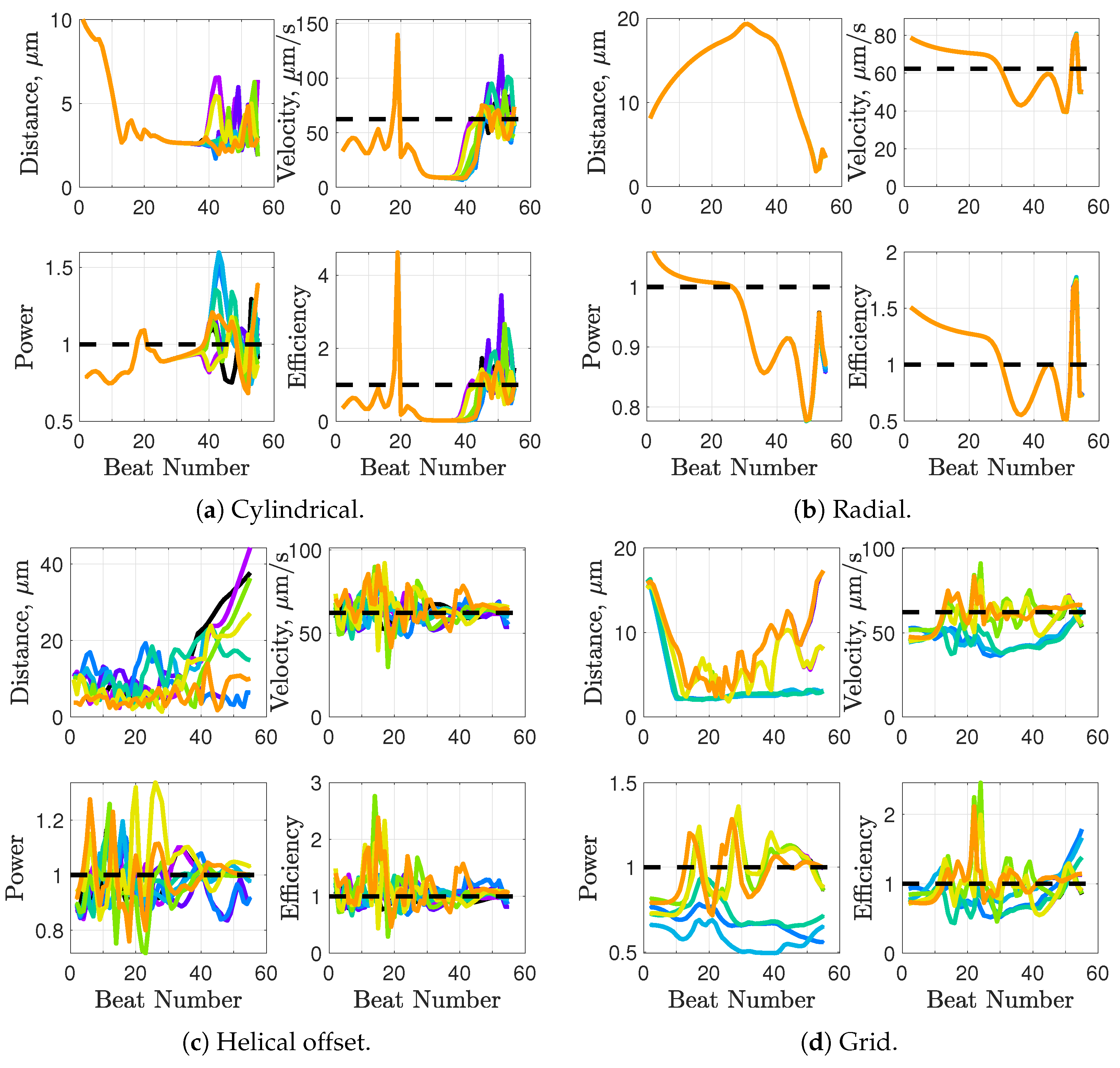
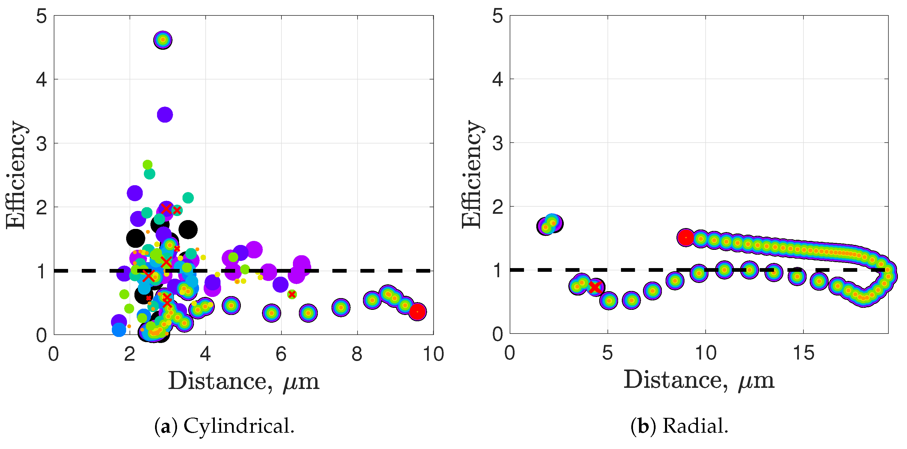
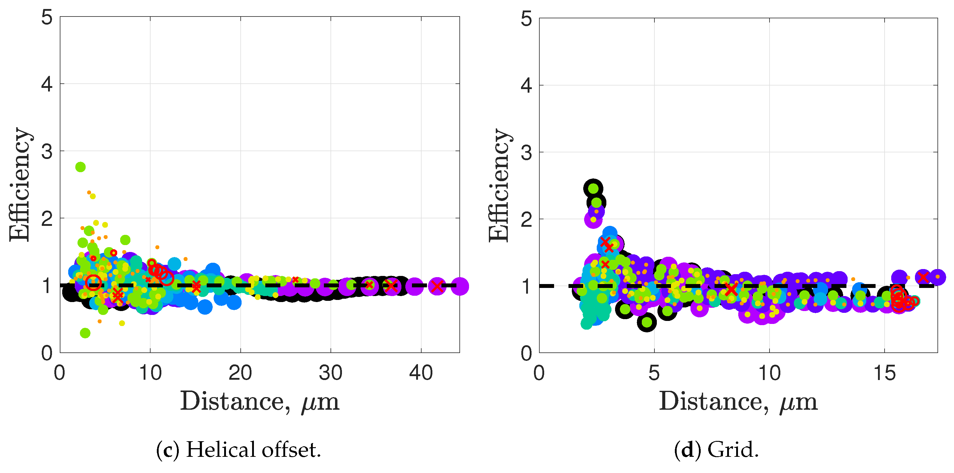
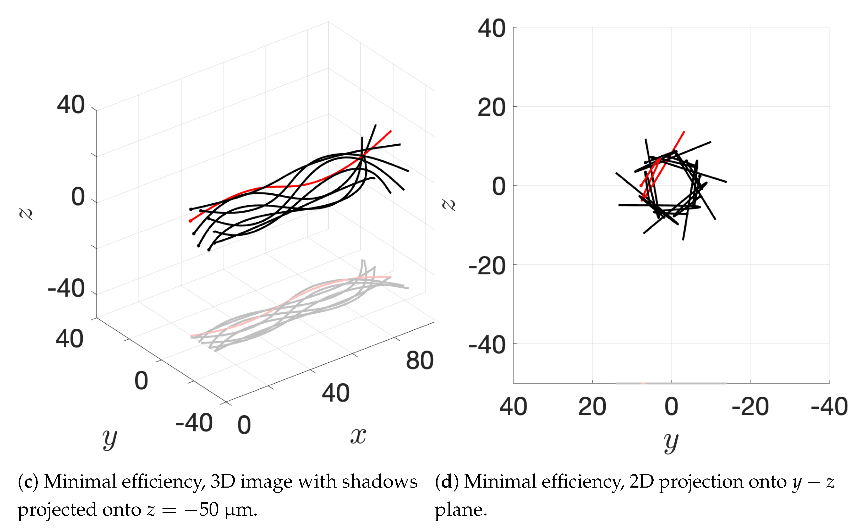
Synchronization and attraction of undulating, planar flagella have been studied for quite some time using both mathematical models and biological experiments. In particular, one theory has been that flagella tend to attract due to energetically favorable conditions, from the perspective of optimizing velocity or efficiency. Our general observations of flagella swimming in groups can be summarized as follows:

• Flagella with similar beat planes tend to attract initially. If their beat planes are identical, attraction is a stable long-term behavior. In all other geometries, attraction is transient.
• If beat planes are nearly identical, velocities and efficiencies decrease as flagella attract.
• Flagella in non-identical beat planes tend to swim apart in the long term.
• Flagella can rotate to have beat planes that are closer to nearby neighbors and this is often accompanied by a transient attraction phase, with decreases in velocities and efficiencies.
• Flagella do not tend to swim in higher efficiency configurations unless there is another mechanism for keeping flagella near one another, such as apical hook binding.
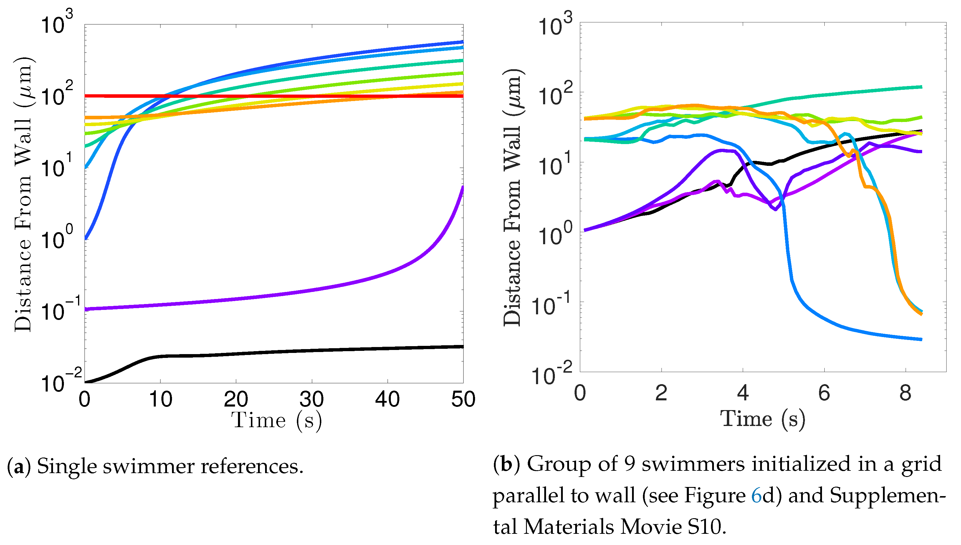
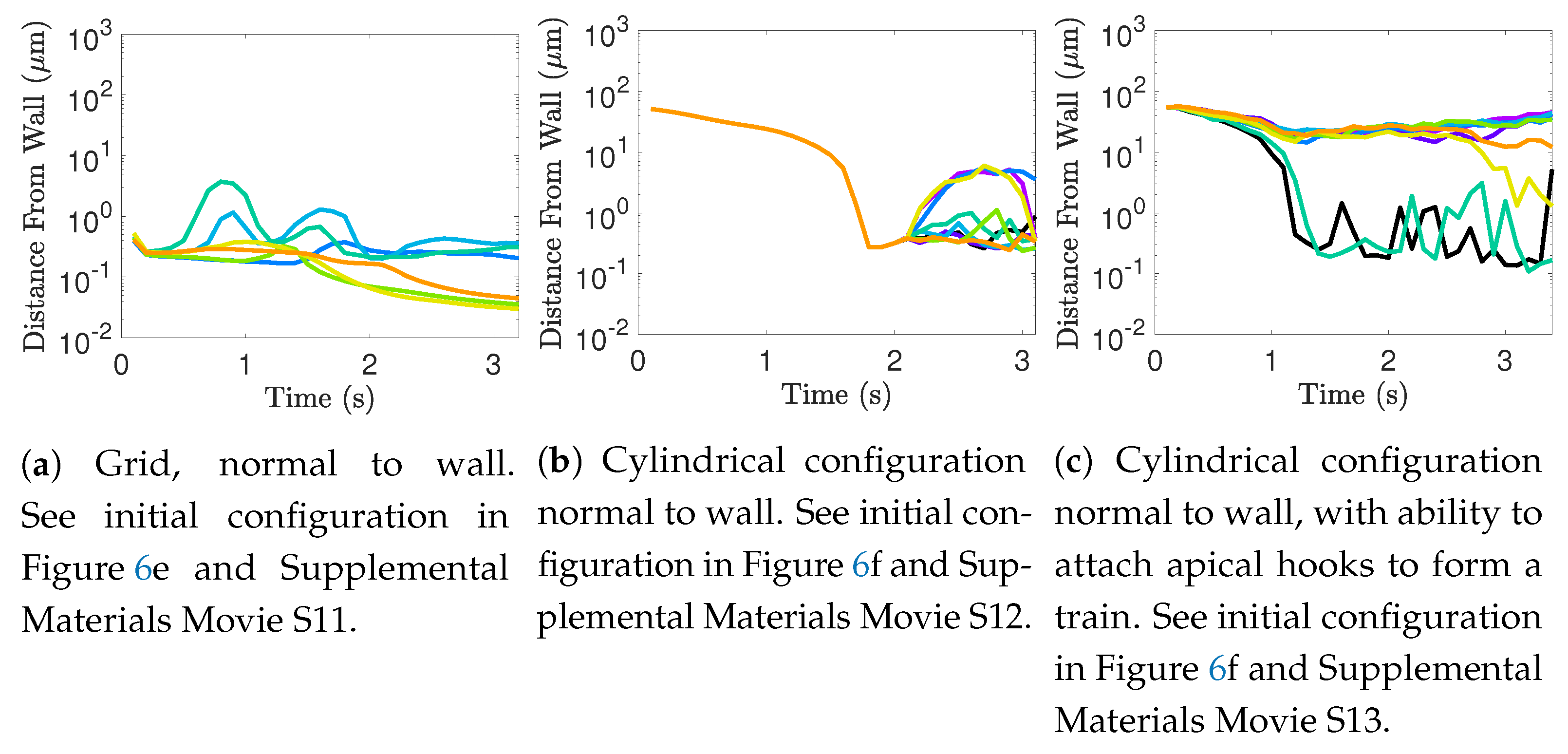
• Near surfaces, having more than one flagella present may promote aggregation unless sperm are able to bind to one another and swim as a collective with higher velocities and powers.

These results are consistent with many prior results for coplanar flagellar geometries. For instance, in [28], a 2D model showed attraction amongst many flagella. A comparison of pairs of coplanar flagella in 2D and 3D fluids was done in [29], in which attraction and synchronization was observed in both fluids, and efficiency as well as velocity were shown to increase in some parameter regimes. In [30], pairwise attraction of flagella was demonstrated in a 2D fluid with a resistance term meant to mimic swimming through a complex fluid containing other cells and polymers, though the question of long-term stability of this attraction was posed due to final configurations of the simulations. The work in [33] also included a 2D framework with large populations of flagella (10–1000) and clustering phenomena were demonstrated, though the clustering was sensitive stochasticity in beat frequencies.

Transient attraction dynamics (followed by divergence in longer timescales) have more recently been observed in a model proposed in [36] which considered two coplanar flagella–a scenario in which our model has been shown to have stable attraction dynamics in prior studies [32]. The flagella in [36] are based on a geometric clutch model instead of the preferred curvature model we present here. This difference in modeling framework might explain the discrepancies between our coplanar results and that of [36]. On the other hand, the authors in [36] observed increases in velocity for sperm that are staggered behind one another. In general, these results are in agreement with our models for flagella that have offset heads (i.e., free-swimming results in from the helical offset configuration shown in Figure 10c and the apical hook/sperm train results shown in Figure 18a), though our flagella are swimming in more complex 3D configurations.

Recent, [35] used 3D simulations to show attraction for a pair of flagella and, intriguingly, a stable steady state configuration for a pair of nearly parallel swimmers using simulation lengths of 20 beats. It is worth noting that in many of our simulations, attraction can be observed in the first 20 beats but the divergent long-term behavior we are presenting here is for beat numbers greater than 50. Moreover, our work goes beyond pairs to consider a larger number of flagella and thus, more degrees of freedom in geometric complexity. Our velocity results are in agreement with [35]: swimming side-by-side in a plane seems to slow swimmers down, but swimming in parallel or nearly parallel planes can increase velocity.

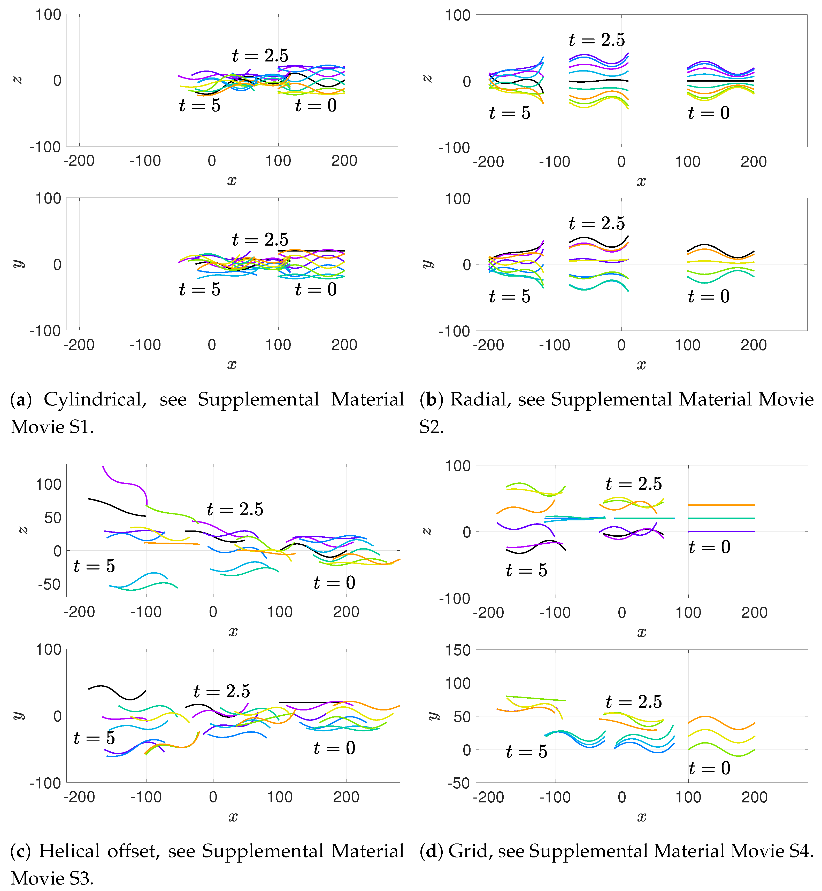
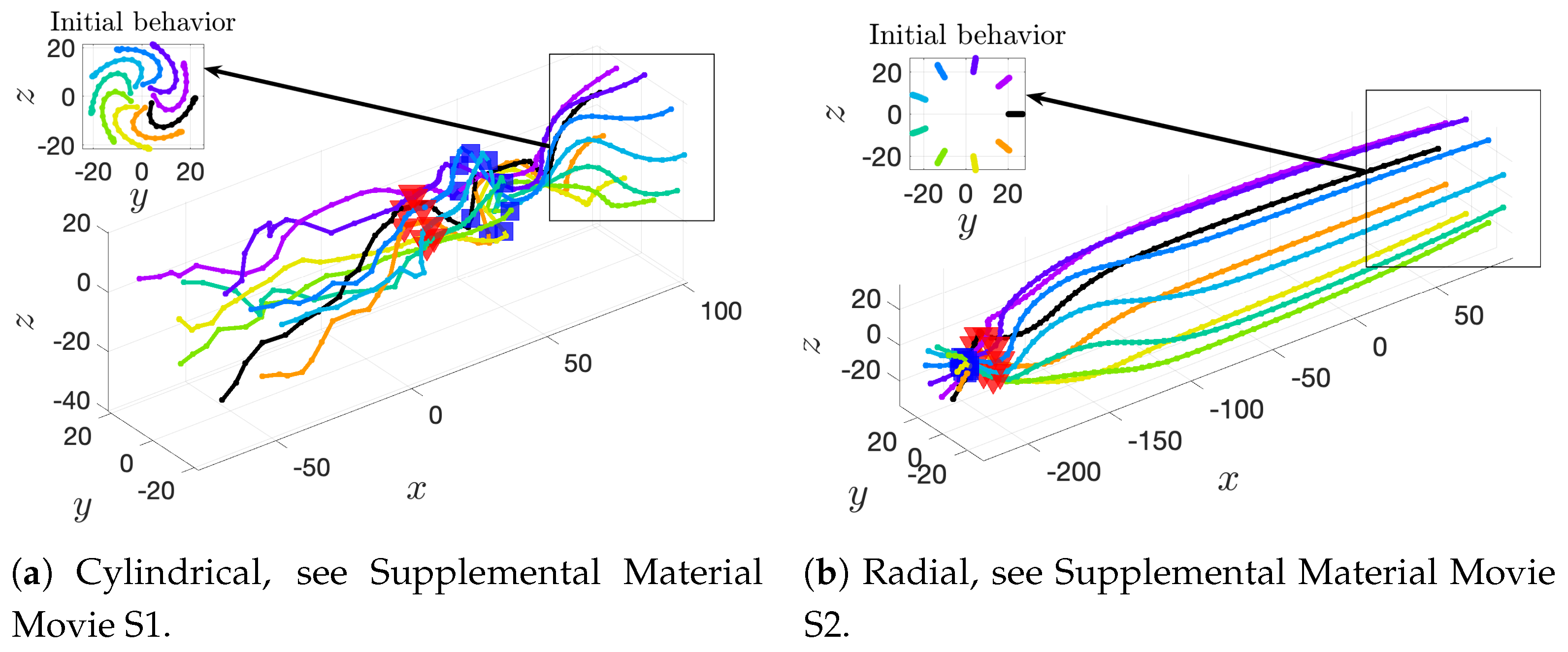
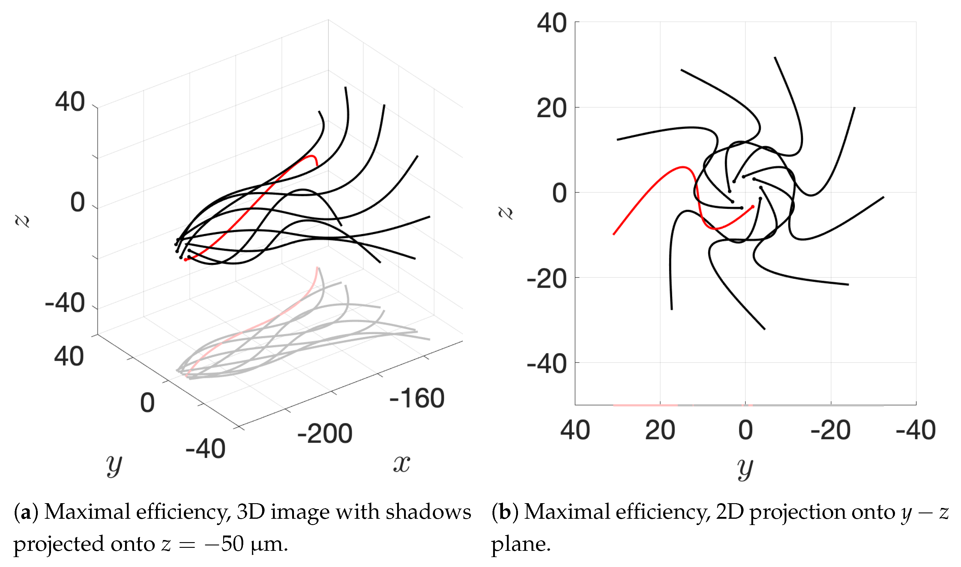
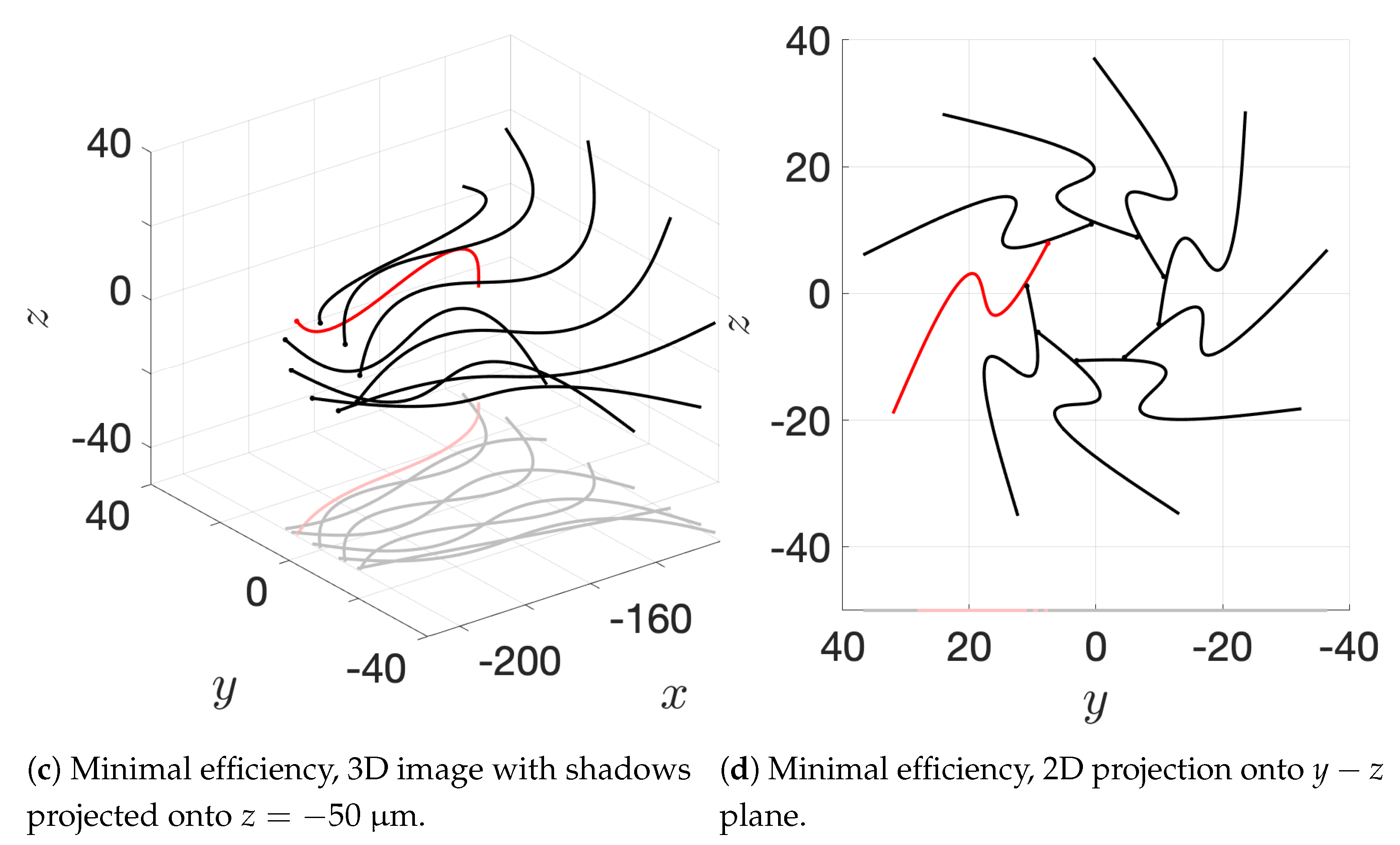
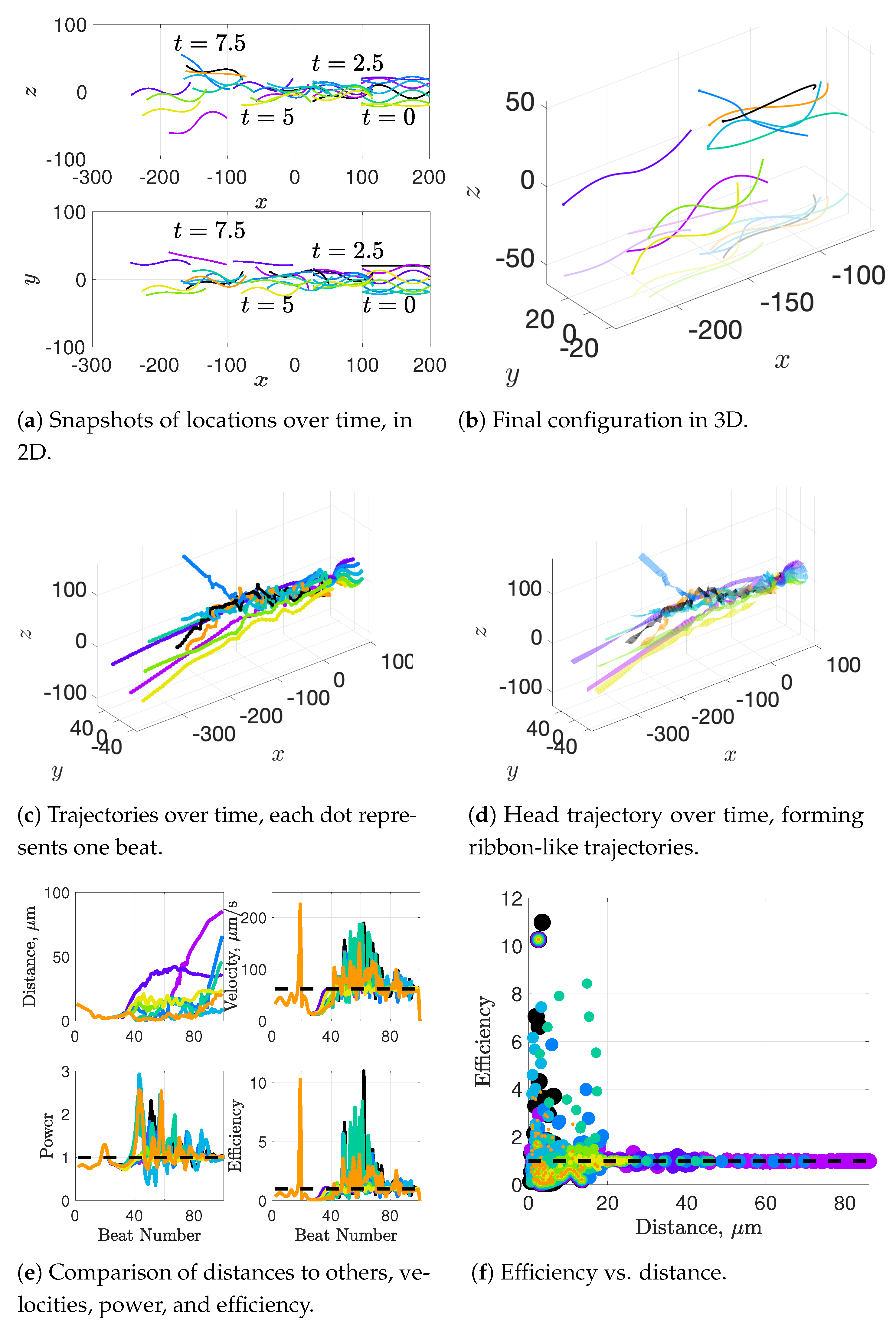
Our results show that flagella swimming in groups will frequently swim in helical or chiral ribbon-like trajectories, despite having a planar flagellar waveform. This is due to hydrodynamic coupling with other nearby flagella and evidence that a non-coplanar waveform is not required for such trajectories. This may provide insight into experimental observations that sperm can swim in helical or chiral ribbon-like trajectories [8,9,10,11], as some have wondered whether results like these indicate a non-planar waveform is more biologically accurate and whether non-planar waveforms are important to sperm motility and function. This work suggests that chiral ribbon trajectories are a natural result of a planar waveform combined with complex 3D fluid–structure interactions, which includes swimming in groups.

Biological settings for sperm involve interactions with surfaces that are complex and can affect motion significantly [20,21,60,61]. While we have not done an exhaustive study of the impact of surfaces in populations of flagella here, our model does indicate that swimming with nearby neighbors can enhance surface accumulation. It is known that flagella attract and accumulate near surfaces, and our results add to the complexity of the picture by considering the role of neighboring flagella in this accumulation process. Further exploration is warranted, particularly given results regarding individual flagella near surfaces. In particular, surface accumulation dynamics can depend on wavenumber [26] and can be modulated by changes in waveform as well as binding dynamics of the sperm heads to epithelial surfaces [24,25,39].

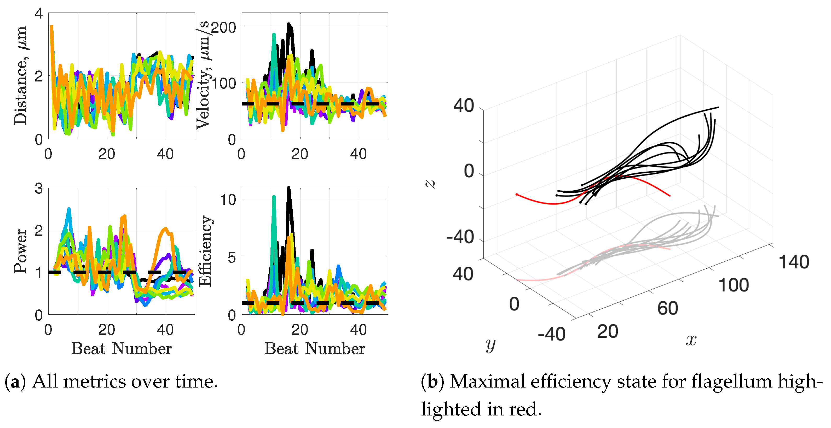
In [43], the authors found that a pair of flagella attached at the head had a small window of geometrical configurations in which both velocity and efficiency were increased beyond that of an individual swimmer. Ultimately, the maximal efficiency configuration coincided with biologically-observed geometries of fused heads of opossum sperm. This paper extends that work to investigate apical hooks as a means for linking sperm flagella. Sperm trains naturally arise, again matching observations but this time in deer mouse sperm in [12].

The authors in [19] found evidence that clustering of sperm is functionally important for fertilization potential and our model demonstrates that there is certainly an advantage to clustering or swimming together in terms of velocity and efficiency. With respect to sperm trains specifically, when we time-average over entire simulations, we observe substantial increases in velocities for sperm trains when compared to individuals. The average velocity of the train of flagella was 15% higher than an individual swimmer with a maximum velocity that was 225% higher than an individual swimmer. Increases of around 50% in velocity were measured in the experimental work [12], so our results underestimate this value but seem reasonable. One reason why we might not fully capture the increases in velocity observed experimentally is that our flagella are idealized to all start in the same phase and cannot modulate this over time. We plan on exploring this in future work. Finally, our model provides efficiency measures that indicate that over the span of our simulation, a train swims on average 50% more efficiently when compared to an individual swimmer. Thus, our model demonstrates that collective swimming can lead to significant hydrodynamic advantages.

5. Conclusions

Flagellar and ciliary transport is necessary for motion in biological systems well beyond the fertility applications discussed here and can only be understood by using a combination of experimental observation and mathematical modeling. For problems at these scales, laboratory measurements of forces, power, and efficiency are difficult, if not impossible, to obtain. Over the last 20 years, the method of regularized Stokeslets [45] has enabled us to effectively model and shed light upon flagellar and ciliary mechanics due to its ease of implementation and the ability to extend the method to a variety blob (regularized delta) functions, control for different levels of desired computational accuracy, incorporate nearby surfaces and effectively study velocities, forces, power, and efficiency simultaneously.

In this paper, we used the method of regularized Stokeslets to show that collective swimming appears to not be a stable long-term behavior of populations of free-swimming flagella exhibiting planar waveforms in a viscous fluid, regardless of velocity and efficiency advantages. If the beat patterns of neighboring flagella are in direct opposition, this may drive flagella apart while velocities and efficiencies are enhanced. If beat patterns of neighboring flagella are more aligned or in sync, then flagella cannot push against each other effectively to swim faster or more efficiently though attraction may occur. Somewhere in between these two behaviors may allow for the most effective propulsion. Increases in velocity and efficiency are most dramatic when flagella are allowed to attach to each other via some physical binding mechanism–and in these cases, the flagella tend to align geometrically to synchronize their beat.

This work is the first to examine collective motion of larger groups of free-swimming flagella with a finer grained model across a large breadth of geometrical configurations over such long timescales. This is also the first model for apical hook binding. Our results also provide the first evidence that helical or chiral-ribbon trajectories can arise not from three-dimensional waveforms but as a consequence long-term interactions with other swimmers. We have also demonstrated strong hydrodynamic evidence for advantages to swimming in a sperm train, and the long-range instability of swimming in groups unless a binding mechanism keeps swimmers close to each other.

The hydrodynamic advantages of collective flagellar motion we have shown here may elucidate evolutionary benefits of sperm morphologies and behaviors in some species. In particular, deer mice that exhibit sperm aggregation or train-like behavior are known to be promiscuous and thus sperm competition may be a primary driver for sperm cooperativity [12]. If competition is high, it makes sense that cooperative mechanisms would arise that enable sperm to swim faster and more efficiently to reach the egg. Even without the complexity of sperm competition, harsh oviductal environments and a short time period of viability for sperm to fertilize the egg also lead to strong evolutionary pressures for sperm to swim quickly and effectively towards the egg.

There are many studies and extensions of this work yet to be done. In particular, there are two fluid assumptions we have made that should be investigated. First, we have assumed a zero Reynolds number, but recent studies of ciliary motion indicate that this simplification may not capture the fluid behavior appropriately [47]. Second, collective swimming has been observed to be important in fluids that are not only viscous, but also elastic [18]. There is also potential to extend this work beyond planar flagellar waveforms into the realm of 3D waveforms such as “Figure 8” deviations or helices observed in some sperm and other flagellated cells. Lastly, understanding flagellar dynamics can provide insight for bioengineered devices–perhaps in the form synthetic cells and devices that can deliver sperm to eggs and aid in overcoming male infertility or, even more broadly, deliver drugs or chemicals to target locations. At the heart of these problems is motion in viscous fluids–a world where inertia has relatively little impact and mathematical models such as the method of regularized Stokeslets may very well hold the key to future developments.

References

1. Macnab, R.M. Bacterial flagella rotating in bundles: A study in helical geometry. Proc. Natl. Acad. Sci. USA 1977, 74, 221–225. [Google Scholar] [CrossRef] [Green Version]
2. Turner, L.; Ryu, W.S.; Berg, H.C. Real-time imaging of fluorescent flagellar filaments. J. Bacteriol. 2000, 182, 2793–2801. [Google Scholar] [CrossRef] [Green Version]
3. Eimers, J.M.; te Velde, E.R.; Gerritse, R.; Vogelzang, E.T.; Looman, C.W.; Habbema, J.D.F. The prediction of the chance to conceive in subfertile couples. Fertil. Steril. 1994, 61, 44–52. [Google Scholar] [CrossRef]
4. Cosson, J.; Huitorel, P.; Gagnon, C. How spermatozoa come to be confined to surfaces. Cell Motil. Cytoskelet. 2003, 54, 56–63. [Google Scholar] [CrossRef]
5. Dresdner, R.; Katz, D. Relationships of mammalian sperm motility and morphology to hydrodynamic aspects of cell function. Biol. Reprod. 1981, 25, 920–930. [Google Scholar] [CrossRef] [Green Version]
6. Vernon, G.; Woolley, D. Basal sliding and the mechanics of oscillation in a mammalian sperm flagellum. Biophys. J. 2004, 85, 3934–3944. [Google Scholar] [CrossRef] [PubMed] [Green Version]
7. Woolley, D.; Vernon, G. A study of helical and planar waves on sea urchin sperm flagella, with a theory of how they are generated. J. Exp. Biol. 2001, 204, 1333–1345. [Google Scholar] [CrossRef]
8. Corkidi, G.; Taboada, B.; Wood, C.; Guerrero, A.; Darszon, A. Tracking sperm in three-dimensions. Biochem. Biophys. Res. Commun. 2008, 373, 125–129. [Google Scholar] [CrossRef]
9. Daloglu, M.U.; Ozcan, A. Computational imaging of sperm locomotion. Biol. Reprod. 2017, 97, 182–188. [Google Scholar] [CrossRef] [PubMed]
10. Su, T.W.; Xue, L.; Ozcan, A. High-throughput lensfree 3D tracking of human sperms reveals rare statistics of helical trajectories. Proc. Natl. Acad. Sci. USA 2012, 109, 16018–16022. [Google Scholar] [CrossRef] [PubMed] [Green Version]
11. Su, T.W.; Choi, I.; Feng, J.; Huang, K.; McLeod, E.; Ozcan, A. Sperm trajectories form chiral ribbons. Sci. Rep. 2013, 3, 1–8. [Google Scholar] [CrossRef] [Green Version]
12. Fisher, H.S.; Hoekstra, H.E. Competition drives cooperation among closely related sperm of deer mice. Nature 2010, 463, 801–803. [Google Scholar] [CrossRef]
13. Hayashi, F. Insemination through an externally attached spermatophore: Bundled sperm and post-copulatory mate guarding by male fishflies (Megaloptera: Corydalidae). J. Insect Physiol. 1996, 42, 859–866. [Google Scholar] [CrossRef]
14. Immler, S.; Moore, H.; Breed, W.; Birkhead, T. By hook or by crook? Morphometry, competition and cooperation in rodent sperm. PLoS ONE 2007, 2, e170. [Google Scholar] [CrossRef] [PubMed] [Green Version]
15. Johnston, S.; Smith, B.; Pyne, M.; Stenzel, D.; Holt, W. One-Sided Ejaculation of Echidna Sperm Bundles. Am. Nat. 2007, 170, E162–E164. [Google Scholar] [CrossRef] [PubMed] [Green Version]
16. Moore, H.; Dvorakova, K.; Jenkins, N.; Breed, W. Exceptional sperm cooperation in the wood mouse. Nature 2002, 418, 174–177. [Google Scholar] [CrossRef] [PubMed] [Green Version]
17. Moore, H.; Taggart, D. Sperm pairing in the opossum increases the efficiency of sperm movement in a viscous environment. Biol. Reprod. 1995, 52, 947–953. [Google Scholar] [CrossRef] [PubMed]
18. Tung, C.; Lin, C.; Harvey, B.; Fiore, A.; Ardon, F.; Wu, M.; Suarez, S. Fluid viscoelasticity promotes collective swimming of sperm. Sci. Rep. 2017, 7, 1–9. [Google Scholar] [CrossRef] [PubMed]
19. Qu, Y.; Chen, Q.; Guo, S.; Ma, C.; Lu, Y.; Shi, J.; Liu, S.; Zhou, T.; Noda, T.; Qian, J.; et al. Cooperation-based sperm clusters mediate sperm oviduct entry and fertilization. Protein Cell 2021, 12, 810–817. [Google Scholar] [CrossRef]
20. Baillie, H.; Pacey, A.; Warren, M.; Scudamore, I.; Barratt, C. Greater numbers of human spermatozoa associate with endosalpingeal cells derived from the isthmus compared with those from the ampulla. Hum. Reprod. 1997, 12, 1985–1992. [Google Scholar] [CrossRef] [Green Version]
21. Ignotz, G.G.; Cho, M.Y.; Suarez, S.S. Annexins are candidate oviductal receptors for bovine sperm surface proteins and thus may serve to hold bovine sperm in the oviductal reservoir. Biol. Reprod. 2007, 77, 906–913. [Google Scholar] [CrossRef] [Green Version]
22. Elgeti, J.; Kaupp, U.B.; Gompper, G. Hydrodynamics of sperm cells near surfaces. Biophys. J. 2010, 99, 1018–1026. [Google Scholar] [CrossRef] [Green Version]
23. Fauci, L.; McDonald, A. Sperm motility in the presence of boundaries. Bull. Math. Biol. 1995, 57, 679–699. [Google Scholar] [CrossRef]
24. Ishimoto, K.; Gaffney, E.A. A study of spermatozoan swimming stability near a surface. J. Theor. Biol. 2014, 360, 187–199. [Google Scholar] [CrossRef]
25. Simons, J.; Olson, S.; Cortez, R.; Fauci, L. The dynamics of sperm detachment from epithelium in a coupled fluid-biochemical model of hyperactivated motility. J. Theor. Biol. 2014, 354, 81–94. [Google Scholar] [CrossRef]
26. Smith, D.; Gaffney, E.; Blake, J.; Kirkman-Brown, J. Human sperm accumulation near surfaces: A simulation study. J. Fluid Mech. 2009, 621, 289–320. [Google Scholar] [CrossRef] [Green Version]
27. Ishimoto, K.; Cosson, J.; Gaffney, E.A. A simulation study of sperm motility hydrodynamics near fish eggs and spheres. J. Theor. Biol. 2016, 389, 187–197. [Google Scholar] [CrossRef] [PubMed]
28. Yang, Y.; Elgeti, J.; Gompper, G. Cooperation of sperm in two dimensions: Synchronization, attraction, and aggregation through hydrodynamic interactions. Phys. Rev. E 2008, 78, 061903. [Google Scholar] [CrossRef] [PubMed] [Green Version]
29. Olson, S.; Fauci, L. Hydrodynamic interactions of sheets vs. filaments: Synchronization, attraction, and alignment. Phys. Fluids 2015, 27, 121901. [Google Scholar] [CrossRef]
30. Jeznach, C.; Olson, S.D. Dynamics of swimmers in fluids with resistance. Fluids 2020, 5, 14. [Google Scholar] [CrossRef] [Green Version]
31. Llopis, I.; Pagonabarraga, I.; Lagomarsino, M.; Lowe, C. Cooperative motion of intrinsic and actuated semiflexible swimmers. Phys. Rev. E 2013, 87, 032720. [Google Scholar] [CrossRef] [Green Version]
32. Simons, J.; Fauci, L.; Cortez, R. A fully three-dimensional model of the interaction of driven elastic filaments in a Stokes flow with applications to sperm motility. J. Biomech. 2015, 48, 1639–1651. [Google Scholar] [CrossRef] [Green Version]
33. Schoeller, S.F.; Keaveny, E.E. From flagellar undulations to collective motion: Predicting the dynamics of sperm suspensions. J. R. Soc. Interface 2018, 15, 20170834. [Google Scholar] [CrossRef]
34. Ishimoto, K.; Gaffney, E.A. Hydrodynamic clustering of human sperm in viscoelastic fluids. Sci. Rep. 2018, 8, 1–11. [Google Scholar] [CrossRef] [Green Version]
35. Walker, B.J.; Ishimoto, K.; Gaffney, E.A. Pairwise hydrodynamic interactions of synchronized spermatozoa. Phys. Rev. Fluids 2019, 4, 093101. [Google Scholar] [CrossRef] [Green Version]
36. Taketoshi, N.; Omori, T.; Ishikawa, T. Elasto-hydrodynamic interaction of two swimming spermatozoa. Phys. Fluids 2020, 32, 101901. [Google Scholar] [CrossRef]
37. Olson, S.D.; Suarez, S.S.; Fauci, L.J. Coupling biochemistry and hydrodynamics captures hyperactivated sperm motility in a simple flagellar model. J. Theor. Biol. 2011, 283, 203–216. [Google Scholar] [CrossRef] [PubMed] [Green Version]
38. Gillies, E.A.; Cannon, R.M.; Green, R.B.; Pacey, A.A. Hydrodynamic propulsion of human sperm. J. Fluid Mech. 2009, 625, 445–474. [Google Scholar] [CrossRef] [Green Version]
39. Curtis, M.; Kirkman-Brown, J.; Connolly, T.; Gaffney, E. Modelling a tethered mammalian sperm cell undergoing hyperactivation. J. Theor. Biol. 2012, 309, 1–10. [Google Scholar] [CrossRef]
40. Wróbel, J.K.; Lynch, S.; Barrett, A.; Fauci, L.; Cortez, R. Enhanced flagellar swimming through a compliant viscoelastic network in Stokes flow. J. Fluid Mech. 2016, 792, 775–797. [Google Scholar] [CrossRef]
41. Ishimoto, K.; Gaffney, E.A. Fluid flow and sperm guidance: A simulation study of hydrodynamic sperm rheotaxis. J. R. Soc. Interface 2015, 12, 20150172. [Google Scholar] [CrossRef] [Green Version]
42. Simons, J.; Fauci, L. A model for the acrosome reaction in mammalian sperm. Bull. Math. Biol. 2018, 80, 2481–2501. [Google Scholar] [CrossRef]
43. Cripe, P.; Richfield, O.; Simons, J. Sperm pairing and measures of efficiency in planar swimming models. Spora J. Biomath. 2016, 2, 5. [Google Scholar] [CrossRef]
44. Fauci, L.J.; Peskin, C.S. A computational model of aquatic animal locomotion. J. Comput. Phys. 1988, 77, 85–108. [Google Scholar] [CrossRef]
45. Cortez, R. The method of regularized Stokeslets. SIAM J. Sci. Comput. 2001, 23, 1204–1225. [Google Scholar] [CrossRef]
46. Ainley, J.; Durkin, S.; Embid, R.; Boindala, P.; Cortez, R. The method of images for regularized Stokeslets. J. Comput. Phys. 2008, 227, 4600–4616. [Google Scholar] [CrossRef]
47. Wei, D.; Dehnavi, P.G.; Aubin-Tam, M.E.; Tam, D. Is the zero Reynolds number approximation valid for ciliary flows? Phys. Rev. Lett. 2019, 122, 124502. [Google Scholar] [CrossRef] [Green Version]
48. Hammer, D.A.; Apte, S.M. Simulation of cell rolling and adhesion on surfaces in shear flow: General results and analysis of selectin-mediated neutrophil adhesion. Biophys. J. 1992, 63, 35–57. [Google Scholar] [CrossRef] [Green Version]
49. Sun, C.; Migliorini, C.; Munn, L.L. Red blood cells initiate leukocyte rolling in postcapillary expansions: A lattice Boltzmann analysis. Biophys. J. 2003, 85, 208–222. [Google Scholar] [CrossRef] [Green Version]
50. Sun, C.; Munn, L.L. Lattice-Boltzmann simulation of blood flow in digitized vessel networks. Comput. Math. Appl. 2008, 55, 1594–1600. [Google Scholar] [CrossRef] [Green Version]
51. Coclite, A.; Mollica, H.; Ranaldo, S.; Pascazio, G.; De Tullio, M.; Decuzzi, P. Predicting different adhesive regimens of circulating particles at blood capillary walls. Microfluid. Nanofluidics 2017, 21, 1–15. [Google Scholar] [CrossRef] [PubMed] [Green Version]
52. Serres, C.; Escalier, D.; David, G. Ultrastructural morphometry of the human sperm flagellum with a stereological analysis of the lengths of the dense fibres. Biol. Cell 1984, 49, 153–161. [Google Scholar] [CrossRef] [PubMed]
53. Cummins, J.; Woodall, P. On mammalian sperm dimensions. Reproduction 1985, 75, 153–175. [Google Scholar] [CrossRef] [PubMed]
54. Ohmuro, J.; Ishijima, S. Hyperactivation is the mode conversion from constant-curvature beating to constant-frequency beating under a constant rate of microtubule sliding. Mol. Reprod. Dev. 2006, 73, 1412–1421. [Google Scholar] [CrossRef]
55. Smith, D.; Gaffney, E.; Gadêlha, H.; Kapur, N.; Kirkman-Brown, J. Bend propagation in the flagella of migrating human sperm, and its modulation by viscosity. Cell Motil. Cytoskelet. 2009, 66, 220–236. [Google Scholar] [CrossRef] [Green Version]
56. Suarez, S.; Dai, X. Hyperactivation enhances mouse sperm capacity for penetrating viscoelastic media. Biol. Reprod. 1992, 46, 686–691. [Google Scholar] [CrossRef]
57. Rothschild. Non-random distribution of bull spermatozoa in a drop of sperm suspension. Nature 1963, 198, 1221. [Google Scholar] [CrossRef]
58. Woolley, D. Motility of spermatozoa at surfaces. Reproduction 2003, 126, 259–270. [Google Scholar] [CrossRef]
59. Boryshpolets, S.; Cosson, J.; Bondarenko, V.; Gillies, E.; Rodina, M.; Dzyuba, B.; Linhart, O. Different swimming behaviors of sterlet (Acipenser ruthenus) spermatozoa close to solid and free surfaces. Theriogenology 2013, 79, 81–86. [Google Scholar] [CrossRef]
60. Smith, T.; Yanagimachi, R. Attachment and release of spermatozoa from the caudal isthmus of the hamster oviduct. J. Reprod. Fertil. 1991, 91, 567–573. [Google Scholar] [CrossRef] [Green Version]
61. Chang, H.; Suarez, S.S. Unexpected Flagellar Movement Patterns and Epithelial Binding Behavior of Mouse Sperm in the Oviduct. Biol. Reprod. 2012, 86, 140. [Google Scholar] [CrossRef] [PubMed]
Figure 1. Images taken from experimental work with sperm swimming in populations. In panel (a), a trajectory of a single human sperm swimming in a population of sperm. The trajectory twists over time, creating a chiral ribbon. Arrow denotes progressive motion of sperm and inset shows a front view of the trajectory. In panel (b), sperm from deer mouse form a sperm train using apical hooks on sperm heads to loop around other flagella. This is one type of collective or cooperative behavior observed in sperm.
Fluids 06 00353 g001
Figure 2. Schematic showing discretization of a flagellum and the forces involved in the model.
Fluids 06 00353 g002
Figure 3. Schematic detailing the sperm train attachment model framework.
Fluids 06 00353 g003
Figure 4. Examples of initial configurations of simulations. For ease of understanding the 3D configurations, we also show the “shadows” of each flagellum on the bottom plane, which is simply a projection of the flagellum onto the z = 50 μ m plane. All units are in μ m and 9 flagella are shown.
Fluids 06 00353 g004
Figure 5. Conceptual idea of configurations between neighboring flagella used to explore the role of phase and alignment. Centerline of each flagella is shown by a dotted line. Rotation of nearest neighbors is done by rotating about this centerline. Beat planes are represented by transparent rectangular shapes either at z = 0 or y = 0 , depending on rotation angle. When these rotations are applied to groups of swimmers in a grid-like formation, the beat planes of neighboring swimmers will either parallel or normal to each other. For cylindrical and radial configurations of groups of swimmers, neighboring swimmers’ beat planes are rotated by an additional 2 π / m for m flagella to maintain circular symmetry.
Fluids 06 00353 g005
Figure 6. Other initial configurations used. Panels (ac) shows phase differences between nearest neighbors. Panels (df) show configurations with a planar surface (wall) at x = 0 . All panels have 9 flagella, with the exception of (a), in which 8 flagella are used to maintain the out of phase pattern amongst nearest neighbors. All units are in μ m.
Fluids 06 00353 g006
Figure 7. Snapshots of locations of flagella over time in 2D, overlaid. Times shown are every 2.5 s (as labeled), equivalent to 25 beats. Head positions started near x = 100 μ m (see Figure 4) and flagella move in the negative x-direction. All units are in μ m. Colors correspond to the flagellum of the same color from the initial configurations in Figure 4.
Fluids 06 00353 g007
Figure 8. Paths of individual flagella over time, by plotting the head position once per beat over the simulation. Insets in panels (a) and (b) show how flagella move in the initial 1.4 s (14 beats) of the simulation. Blue squares denote the location of flagellum head where maximal efficiency is achieved and red triangles denote where minimal efficiency is achieved. Head positions start at x = 100 μ m and flagella move in the negative x-direction, so flagellum heads start at the far right and end in the far left of each image. All units are in μ m. Colors of curves correspond to the flagellum of the same color from the initial configurations in Figure 4.
Fluids 06 00353 g008
Figure 9. Ribbon path trajectories created by triangulation of head positions over each beat for the entire simulation. Due to the lateral oscillation of the flagellum head (initial point) within each beat, the head carves out a ribbon-like trajectory. This ribbon indicates the flagellar beat plane. Blue squares denote the location of flagellum head when maximal efficiency is achieved and red triangles denote the location of the flagellum head when minimal efficiency is achieved. Head positions start near x = 100 μ m and flagella move in the negative x-direction, so flagella heads start at far right and end up in the far left of each image. All units are in μ m. Colors of ribbons correspond to the flagellum of the same color from the initial configurations in Figure 4.
Fluids 06 00353 g009
Figure 10. Comparison of minimal distances to neighboring flagella (upper left plot in each panel), velocities (average path velocities), power, and efficiency in reference to an individual swimmer in free space (dotted line). Note that power and efficiency have been normalized in reference to an individual swimmer in free space. Colors of curves correspond to the flagellum of the same color from the initial configurations in Figure 4.
Fluids 06 00353 g010
Figure 11. Efficiency normalized to a single swimmer in free space (dotted horizontal line), plotted with respect to minimal distance (in μ m) to other flagella. Each dot represents one flagella (corresponding to its color as depicted in Figure 4) for one beat. Dot size is used to effectively show overlap of data only and does not indicate any other metric. For reference, red circles denote initial beat and red x’s denotes final beat for each flagella, with label size varied to show overlap.
Fluids 06 00353 g011aFluids 06 00353 g011b
Figure 12. Snapshots of flagellar configurations for the cylindrical simulation from Figure 4a, for both maximal and minimal efficiencies observed. One flagellum is highlighted in red for visual emphasis of the geometry. See Supplemental Material Movie S1 for all configurations over time.
Fluids 06 00353 g012aFluids 06 00353 g012b
Figure 13. Snapshots of flagellar configurations for the radial simulation from Figure 4b, for both maximal and minimal efficiencies observed. One flagellum is highlighted in red for visual emphasis of the geometry. See Supplemental Material Movie S2 for all configurations over time.
Fluids 06 00353 g013aFluids 06 00353 g013b
Figure 14. Phase/alignment differences between nearby neighbors. Snapshots of locations of flagella over time in 2D, overlaid. Times shown are every 2.5 s or 25 beats, as labeled in panels. Head positions started near x = 100 μ m (see Figure 6a–c) and flagella move in the negative x-direction. All units are in μ m. Color of curves indicates data for flagellum of matching color from initial configurations (see Figure 6a–c).
Fluids 06 00353 g014
Figure 15. Phase/alignment differences between nearby neighbors, ribbon path trajectories created by triangulation of head positions over each beat for the entire simulation. Due to lateral oscillation of head within each beat, the head carves out a ribbon-like surface indicating the flagellar beat plane. Blue squares denote the location of flagellum head when maximal efficiency is achieved and red triangles denote the location of the flagellum head when minimal efficiency is achieved. Head positions started near x = 100 μ m and flagella move in the negative x-direction, so flagella heads start at far right and end up in the far left of each image. All units are in μ m. Color of curves indicates data for flagellum of matching color from initial configurations (see Figure 6a–c).
Fluids 06 00353 g015
Figure 16. Phase differences between nearby neighbors. Comparison of minimal distances to other flagella, velocities, power, and efficiency with reference to individual swimmer in free space (dotted line). Color of curves indicates data for flagellum of matching color from initial configurations (see Figure 6a–c). Note that panels (a,b) only have 8 curves in order to exploit symmetries of rotation.
Fluids 06 00353 g016
Figure 17. Positions of flagella in sperm train model, starting from the cylindrical initial configuration depicted in Figure 4a. All units are in μ m. Panel (a) shows 2D snapshots of locations of flagella over time in 2D, overlaid. Times shown are every 2.5 s or 25 beats. Initial and middle time points are shown in lighter colors, with the initial configuration to the far right. Final time point positions are shown in bolder colors towards the left. Head positions started near x = 100 μ m and flagella move in the negative x-direction. Panel (b) shows the positions of flagella at the end of the simulation, forming a phase-locked train. See Supplemental Material Movie S9.
Fluids 06 00353 g017
Figure 18. Comparison of minimal distances to other flagella, velocity, power and efficiency of apical hook model. In panel (a), we see all metrics plotted over time. Color of curves indicates data for flagellum of matching color from the initial configuration, shown in Figure 4a. In panel (b), we show the configuration for maximal efficiency of the leading flagellum.
Fluids 06 00353 g018
Figure 19. Distance between the head point of the flagellum and the wall over time for swimmers initialized in parallel planes to the wall. In (a), individual flagella are initialized at various heights away from the wall, with the flagellar beat plane parallel to the wall (each curve is a simulation of one solitary flagellum and results are overlaid). All flagella tend to move away from the wall over time, regardless of how far they start from the wall. In (b), we show the results of a single simulation of a group of 9 flagella, all initiated with beat planes parallel to the surface, in phase but separated from each other by a distance of 20 μ m. Here, positions of heads are plotted once per beat to remove the zig-zag pattern that can occur due to the periodic undulation of flagella (1 beat = 0.1 s). Notice that some sperm seem to become trapped near the wall, in contrast with the individual swimmers in panel (a). Color of curves in panel (b) indicates data for flagellum of matching color from Figure 6d.
Fluids 06 00353 g019
Figure 20. Distance between the head point of the flagellum and the wall over time for 9 swimmers initialized in planes normal to the wall. In panel (a), we show swimmers initialized in a grid but with planes normal to the wall. Here, as expected, we see the swimmers moving mostly towards the wall over time. We can contrast that with panel (b), which are also initialized in planes normal to the wall but the flagella are in a cylindrical configuration, as in Figure 6f. Lastly, panel (c) shows the results of swimmers initialized in a cylindrical configuration, as in Figure 6f, but with the ability to “hook” onto each other and form a train. Again, they initially swim towards the wall, but some swim away after about 1 s, or 10 beats. Color of curves indicates data for flagellum of matching color from Figure 6e–f.
Fluids 06 00353 g020
Publisher’s Note: MDPI stays neutral with regard to jurisdictional claims in published maps and institutional affiliations.