Article

A Hybrid Parallel Numerical Model for Wave-Induced Free-Surface Flow

by
Georgios A. Leftheriotis
1,
Iason A. Chalmoukis
1,
Guillermo Oyarzun
2 and
Athanassios A. Dimas
1,*
1
Department of Civil Engineering, Campus Rio, University of Patras, 26500 Patras, Greece
2
Barcelona Supercomputing Center, 08034 Barcelona, Spain
*
Author to whom correspondence should be addressed.
Fluids 2021, 6(10), 350; https://doi.org/10.3390/fluids6100350
Submission received: 6 September 2021 / Revised: 29 September 2021 / Accepted: 1 October 2021 / Published: 4 October 2021
(This article belongs to the Special Issue Theory and Applications of Ocean Surface Waves)

Abstract

:
An advanced numerical model is presented for the simulation of wave-induced free-surface flow, utilizing an efficient hybrid parallel implementation. The model is based on the solution of the Navier–Stokes equations using large-eddy simulation of large-scale coastal free-surface flows. The three-dimensional immersed boundary method was used for the enforcement of the no-slip boundary condition on the bed surface. The water-air interface was tracked using the level-set method. The numerical model was effectively validated against laboratory measurements involving wave propagation over a flatbed with an elliptical shoal, whose presence induces combined wave refraction and diffraction phenomena. The parallel implementation of the model enabled the efficient simulation of depth-resolved, wave-induced, three-dimensional, free-surface flow; the model parallel efficiency and strong scaling are quantitatively demonstrated.

1. Introduction

During the last decades, the development of computer technology has advanced, and, consequently, the computing power has increased significantly. As a result, numerical modeling has become increasingly popular in coastal research. More specifically, computational fluid dynamics (CFD) is one of the branches of fluid mechanics with the potential to fully exploit modern computer technologies. Moreover, taking into consideration the effect of climate change and the increased wave heights, coastal environments are becoming more and more vulnerable to erosion and flooding phenomena. Thus, the use of numerical models is more than ever mandatory to achieve realistic simulations of the wave field and understand in more detail the hydrodynamics in coastal zones.
Many numerical models have been developed to study nearshore wave processes. Depth-integrated models utilizing the Boussinesq-type equations are quite popular for the numerical modeling of waves [1,2]. Boussinesq-type models (BTMs) provide an effective way to compute the free-surface flow in cases of a nearly uniform vertical distribution of flow variables. However, BTMs contain high-order, partial-derivative terms whose accurate discretization is rather difficult and increases the computational cost. Moreover, in phenomena with strong spatial variability of the flow field in the vertical direction, which is the case in coastal zones, three-dimensional (3D) modeling is more appropriate than the depth-averaged one [3].
Apart from the BTM, another popular approach is the development of one- or two-layer depth-integrated non-hydrostatic wave models [4,5,6,7]. In this specific approach, the vertical flow structures are indirectly resolved in the governing equations. However, additional layers should be incorporated in the non-hydrostatic models to increase the order of accuracy. Multilayer non-hydrostatic models can resolve more complex flow structures over the water column, and they can represent more accurate coastal wave processes [8]. Nevertheless, to accurately capture the 3D effects of the coastal processes that intertwine in the nearshore zone, fully 3D numerical models are needed.
Navier–Stokes equations can theoretically describe most fluid problems with reasonable accuracy. The performance of direct numerical simulation (DNS) using the Navier–Stokes equations is highly impractical for high Reynolds number problems, due to computer power restrictions. There are two popular alternatives for simulating large-scale cases. The first alternative is to use the Reynolds-averaged Navier–Stokes (RANS) equations, and the second alternative is to use large-eddy simulation (LES). LES is a widely used methodology for the numerical simulation of high Reynolds number turbulent flows. In the LES approach, the flow structures are separated into large and small eddies. The large eddies are explicitly solved for, while the small eddies are parametrized with the use of a subgrid-scale (SGS) model [9].
Several numerical studies for coastal flow simulation have been presented in recent years utilizing high-performance computing (HPC). Önder and Yuan [10] performed DNS of oscillatory flow over a rippled bottom in order to study in detail the 3D features of the flow in fully turbulent regimes. They used the message passage interface (MPI) for the parallel implementation of their code. Very fine grid resolution was employed, with grid spacing in the order of the Kolmogorov scale. Thus, they were able to fully resolve all flow features and the wave boundary layer, concluding that the flow is characterized by the formation of two dominant large-scale vortices. Oyarzun et al. [11] presented a 3D numerical model using the LES approach, implemented to run in both CPU and GPU systems. An MPI + OpenACC strategy was followed in order to increase the computational performance. The oscillatory flow was simulated over a fixed rippled bed for large-scale Reynolds numbers (Re = 2 × 10⁵). They concluded that for accurate prediction of flow parameters in coastal flows, the numerical simulations should be performed at Reynolds numbers as close as possible to the original ones. Jin et al. [12] performed 3D LES in order to simulate oscillatory flow over fixed ripples. The MPI protocol was utilized for the parallel implementation of the code. Due to the use of HPC, they performed high-resolution numerical simulations, and they managed to visualize the evolution of rib patterns during a flow cycle.
Using the projection method for the numerical solution of the Navier–Stokes equations, the most time-consuming part of the algorithm is the numerical solution of the Poisson equation for pressure. For one-fluid cases, the matrix of the linear system resulting from the spatial discretization of the Poisson equation has constant coefficients; therefore, efficient fast direct solvers (FDSs) are used, which take advantage of fast Fourier transforms (FFT). For flows with an air-water interface, the Poisson equation matrix has varying coefficients in space and time because the density field varies spatially and temporarily in the vicinity of the interface; therefore, the direct application of an FDS is not possible. Recently, Frantzis and Grigoriadis [13] and De Vita et al. [14] used the indirect FDS approach in Dodd and Ferrante [15] to simulate free-surface flows induced by the interaction of waves with stationary or moving solid bodies. Another alternative for the variable-coefficient matrix issue is the use of iterative solvers but they are usually much slower than the indirect FDS. To overcome this drawback, in the present work, a fast iterative solver was developed utilizing parallel architectures and HPC systems.
To summarize, the constant improvement of computer power during the last decade allowed the researchers to simulate 3D coastal processes close to bed at prototype experimental or physical scales, using HPC. However, to the authors’ knowledge, the use of 3D LES to resolve the whole water column, from the bed to the free surface, during wave propagation, is still limited. Considering that the numerical solution of the incompressible Navier–Stokes equations provides an accurate prediction of hydrodynamics, the scope of the present study is the development and validation of a fully 3D numerical model to simulate flow processes induced by wave refraction and diffraction. This will enable us to study, apart from the wave transformation that a BTM or a depth-averaged non-hydrostatic model can simulate, the complete 3D flow field. In order to use the specific approach for realistic-scale situations at high Reynolds numbers, very fine spatial discretization is needed, which leads to extremely high computational costs. For the above-mentioned reasons, the present numerical model is utilizing HPC. A hybrid parallel methodology is proposed, which includes an MPI + OpenMP implementation that can efficiently take advantage of modern supercomputing capabilities.

2. Materials and Methods

2.1. Methodology

In the present numerical model, the flow in the water and the air was modeled as one-fluid flow governed by the 3D incompressible Navier–Stokes equations in non-dimensional form.
u i x i = 0
u i t + x j ( u i u j ) = 1 ρ p x i τ i j x j + 1 ρ 1 Re x j ( μ ( u i x j + u j x i ) ) + δ i 3 Fr 2 + f i
where ui are the velocity components, xi are the Cartesian coordinates (x1 is the streamwise, x2 is the spanwise, and x3 is the vertical coordinate opposite to gravity), t is the time, ρ is the one-fluid density normalized by the water density, p is the total pressure, τij are the SGS stresses related to LES, Re is the Reynolds number, μ is the one-fluid dynamic viscosity normalized by the water dynamic viscosity, δ is the Kronecker’s delta, Fr is the Froude number, and fi is a source term associated with the implementation of the immersed boundary (IB) method. In the present work, the 3D implementation of the IB method [16] was utilized for the enforcement of the no-slip boundary condition on the bed surface. The SGS stresses were modelled by the standard eddy-viscosity Smagorinsky model [9]. In Equation (2), lengths are non-dimensionalized by a characteristic depth, d, and velocities by (gd)1/2; therefore, Re = d(gd)1/2/νw, and, Fr = 1, where νw is the water kinematic viscosity.
The spatial discretization of all equations is performed using 2nd order central finite differences on a Cartesian grid, an advantage that is afforded using the IB method for the imposition of the no-slip boundary condition since the bed does not have to coincide with the numerical grid. Not using boundary conforming grids results in a substantial increase in the performance and efficiency of the HPC tools.
The temporal discretization is based on the time-splitting projection method where all terms of Equation (2), except the pressure term, are treated explicitly using a 2nd order Adams–Bashforth scheme for the computation of an intermediate velocity uim+1/2. The final velocity field uim+1 is obtained by the pressure gradient as follows:
u i m + 1 = u i m + 1 / 2 Δ t ρ p m + 1
The present approach, in terms of the application of the projection method, is highly encountered in the literature for the solution of the incompressible Navier–Stokes equations. In Equation (3), the pressure is computed by the numerical solution of the corresponding Poisson equation
( 1 ρ p m + 1 ) = 1 Δ t u i m + 1 / 2
at each numerical time step.
The evolution of the free surface is based on the level-set method [17], following the advection equation, expressed as
φ t + u i φ = 0
where φ is a signed distance function, defined to be equal to zero at the level of the free surface.
The incident waves are generated at the left boundary of the computational domain by resembling numerically the action of a piston-type wavemaker on the left boundary. To achieve that, the horizontal velocity was imposed there, following the relationship [18]
u 0 ( t ) = 1 2 S 0 ω cos ( ω t π / 2 ) + 1 16 H 0 2 d 0 ω ( 3 cosh ( k d 0 ) sinh 3 ( k d 0 ) 2 S 0 H 0 ) cos ( 2 ω t π )
where H0 is the wave height, k = 2π/λ is the wavenumber, λ is the wavelength, d0 is the water depth at the wavemaker, and S0 is the stroke of the wavemaker, given by
S 0 = H 0 sinh ( 2 k d 0 ) + 2 k d 0 4 sinh 2 ( k d 0 )
To avoid undesired wave reflections from the boundaries of the computational domain, sponge layer regions have been implemented in both streamwise boundaries, following the method proposed in Jacobsen et al. [19]. For further details on the methodology implementation, the interested reader is referred to Dimas and Koutrouveli [18] and Koutrouveli and Dimas [20]. The structure of the whole algorithm is presented in Table 1.

2.2. Parallel Implementation

The parallelization of the numerical code utilizes a hybrid MPI + OpenMP approach. This parallel implementation relies on dividing the computational domain into N non-overlapping and equally distributed subdomains. Each MPI process performs calculations only on the cells of its associated subdomain. Additionally, an external layer of cells, so-called halo cells, must be attached to each subdomain. These cells are replica values of the neighboring cells coupled with the subdomain. The purpose of these cells is to maintain the coherence of the numerical results among the whole domain. Therefore, MPI communications must update the halo cells when their values change on their origin subdomain. These MPI commands are point-to-point communications (MPI_Isend and MPI_Irecv) since they only link neighboring subdomains. The number of halo layers required to perform the local calculations depends on the discretization scheme. In our implementation, stages from 1 to 4 (Table 1) are based on a second-order discretization that only requires one layer of halo cells. However, the interface tracking utilized in stage 5 (Table 1) requires three layers of halo cells, thus increasing the communication cost of updating the unknowns associated with that operation. Figure 1 exemplifies the halo layer on a two-dimensional (2D) subdomain of 6 × 6 cells. At the left side of Figure 1, a sketch of a single halo layer required for a second-order discretization is presented; at the right side of Figure 1, a sketch of three halo layers necessary for the interface tracking is presented. This configuration is easily extrapolated to 3D formulations. More details can be found in Oyarzun et al. [11].
The operations within the local domains are represented with three nested loops that sweep the three directions of the local Cartesian domain (x1, x2, and x3). The iterations performed within these loops are independent of each other. This feature favors the utilization of loop-based shared memory parallelization, such as OpenMP. In our case, each MPI process launches many OpenMP threads that perform the calculations in parallel. The MPI process is associated with a CPU socket, and the OpenMP threads are linked with each core of that socket.

2.3. Parallelization of the Pressure Solution

Regarding the computation of the pressure field, iterative methods are the only plausible choice for solving such large-scale linear systems. Krylov subspace methods are the most commonly used solvers for calculating the pressure field from the linear system [21,22]. Two-phase simulations generate a Poisson equation (Equation (4)) that its matrix is asymmetric and with coefficients that change after each time integration step due to the temporal variation of the flow density as a function of the free-surface movement. Therefore, the biconjugate gradient method (BiCG) is the most suitable for its solution. The BiCG algorithm is composed of the sparse matrix–vector product (SpMV) and vectorial operations. The implementation of these linear algebra operations consists of a loop over the matrix rows or vector components. The loop independence on these operations makes them compatible with our OpenMP parallelization. Additionally, the SpMV requires a halo update before being applied, thus requiring point-to-point MPI communications (MPI_Isend and MPI_IRecv) of one layer of cells. The dot product is the only vector operation that involves communications. First, each subdomain calculates its local dot product, and then a collective all-to-all communication (MPI_Allreduce) is needed to perform the global sum and to store the result on each process. Within the iterative loop of the solver, the SpMV is called twice while the dot product is computed five times. The solver performs hundreds of iterations to converge; therefore, these two operations determine the simulation scalability.
The previous solution of the pressure is utilized as the starting point of the iterative process. However, since the coefficients of the matrix and the right-hand side of Equation (4) change after each time integration step, the iterative process is rarely stabilized within few iterations. A Jacobi preconditioner reduces the iterations at a low cost since its application is equivalent to a vectorial operation. Moreover, this preconditioner is suitable for the MPI + OpenMP implementation since it is loop based and does not demand communications.

3. Results

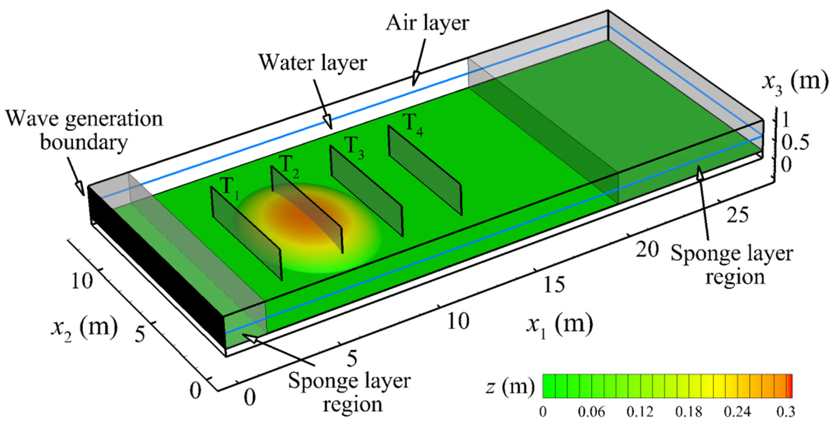
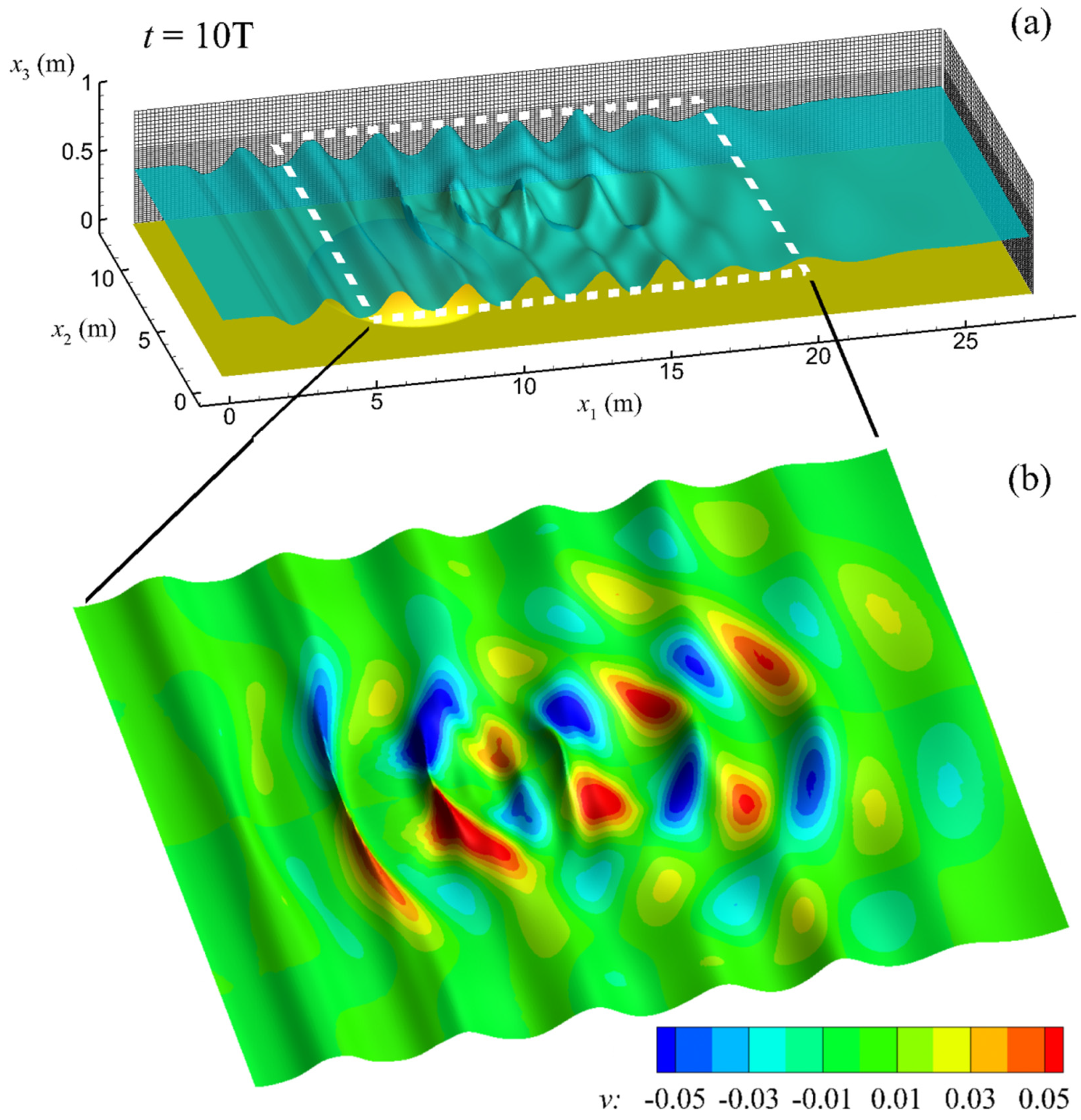
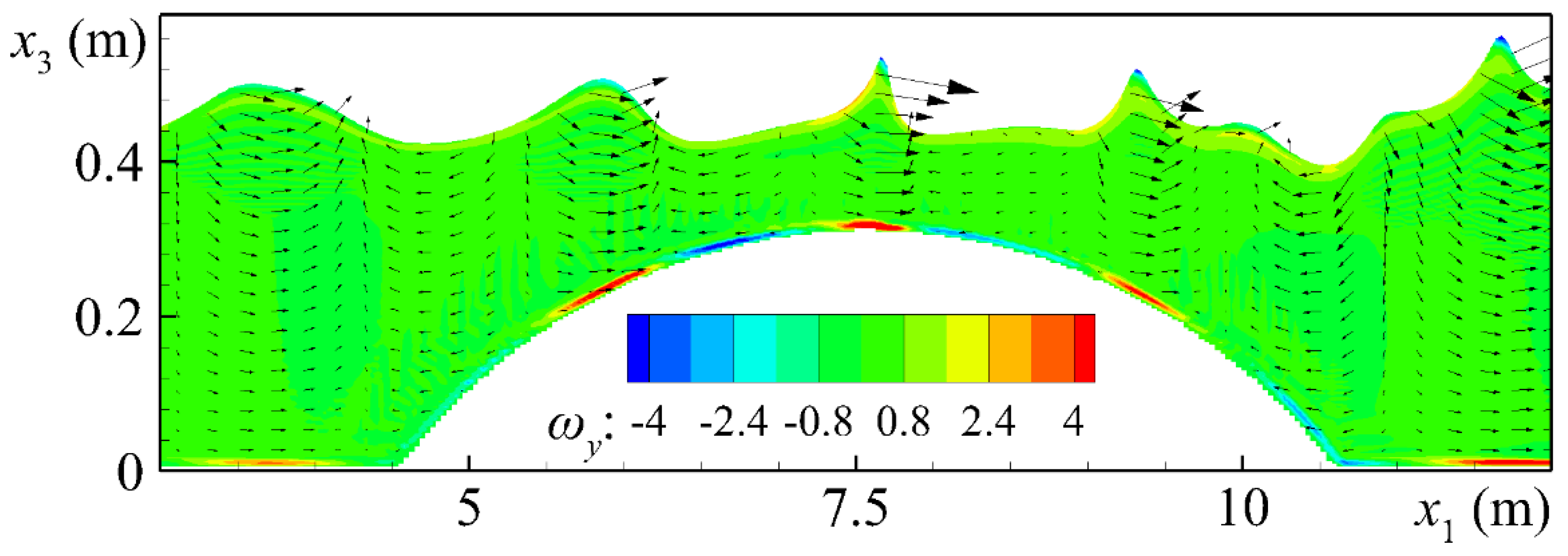
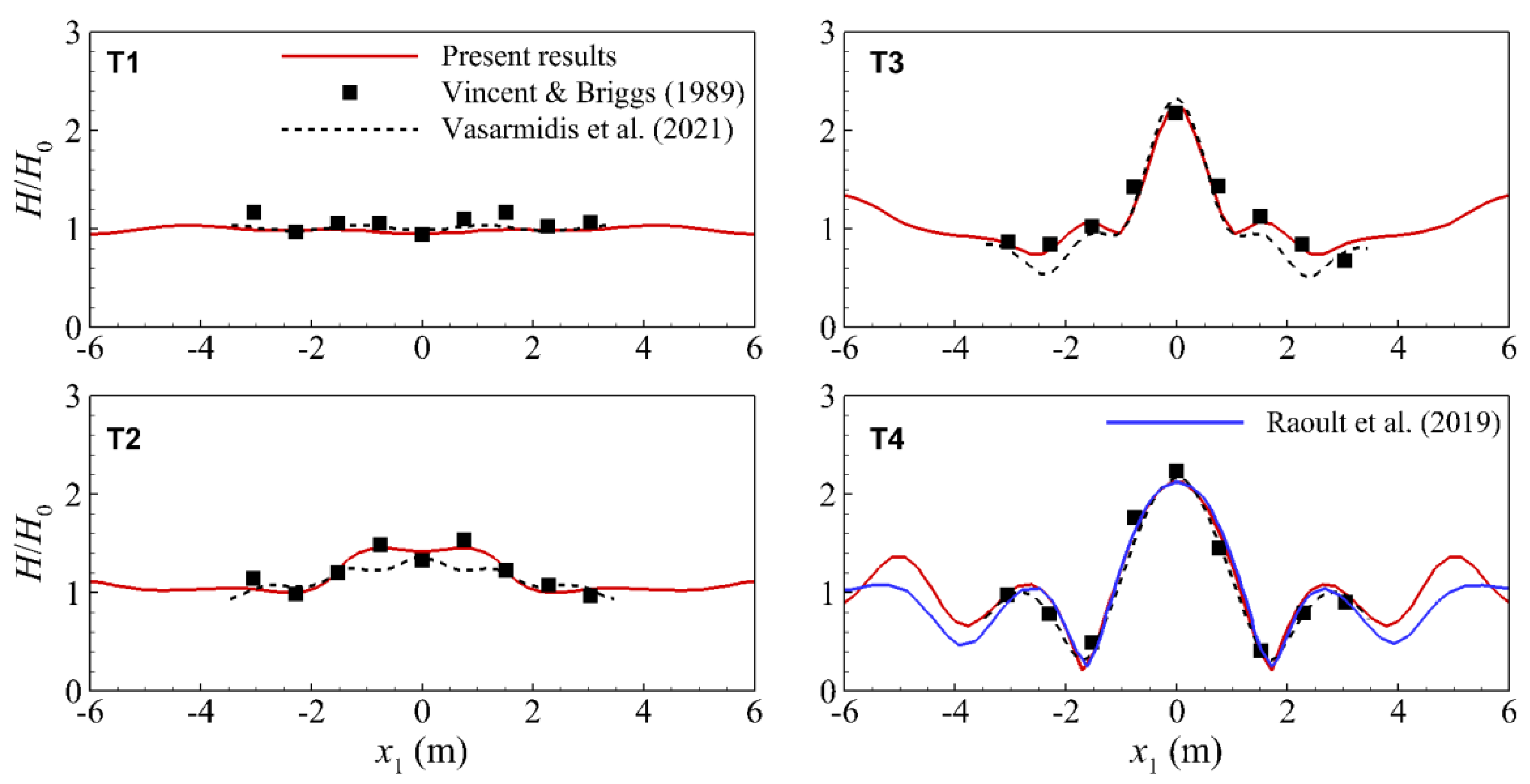
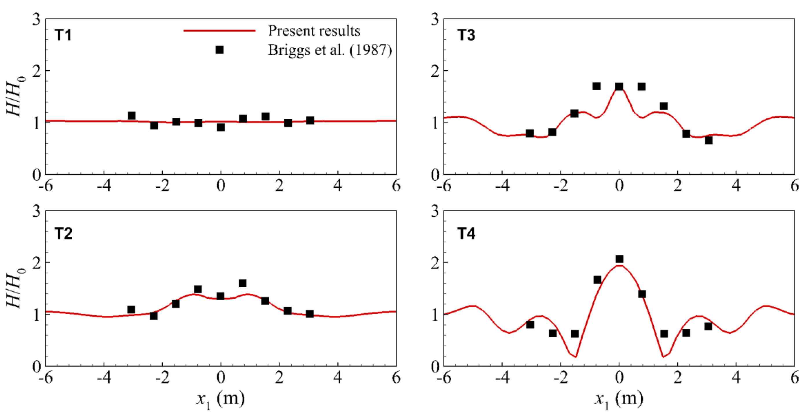
3.1. Waves Propagation over an Elliptical Shoal

Experimental measurements of regular and irregular waves propagation over a submerged elliptical shoal were presented in Briggs [23] and Vincent and Briggs [24]. To validate the present numerical model, two benchmark cases of regular waves were selected to demonstrate the ability of the model to simulate complex 3D wave transformations due to the simultaneous effects of wave refraction and diffraction. This experiment has also been reproduced by 2D depth-integrated, non-hydrostatic models for the simulation of coastal waves over varying bathymetries [25,26,27]. It should be noted that the performance of the above mentioned models was good, but they underestimated the wave height behind the shoal. Additionally, a simulation using a 2D fully non-linear BTM was performed by Viviano et al. [28] with similar accuracy. Depth-averaged models can handle very efficiently several nearshore phenomena, such as wave refraction and diffraction. However, when aiming at modeling the nearshore flow field, their weakest point is their inability to resolve the velocity and pressure fields along the depth. To face this problem, numerical simulations of the 3D Navier–Stokes equations should be performed as in Ha et al. [29]. A more recent study was also presented by Raoult et al. [30] after solving the 3D Euler–Zakharov equations. However, in both studies, only free-surface elevation results were presented but no velocity or vorticity ones. To the authors’ best knowledge based on the recent literature, the present article is the first to present and discuss the results of the 3D velocity field for the experiments in Briggs [23] and Vincent and Briggs [24].
The experiments were conducted in a directional wave basin with width, 35 m, and length, 29 m. The measurements were obtained in an area 6.10 m wide and 15.24 m long around the shoal. The elliptical shoal was designed based on the work in Berkhoff et al. [31], with a major radius of 3.96 m and a minor radius of 3.05 m. The perimeter of the shoal boundary was defined as
( X 3.05 ) 2 + ( Y 3.96 ) 2 = 1
where X and Y are the axes of a local coordinate system positioned at the center of the elliptical shoal. The bed level outside the shoal area was flat, at a constant water depth of d = 0.4572 m (18”), while the shoal surface level, ds, was defined by the following expression:
d s = 0.4572 + 0.7620 [ 1 ( X 3.81 ) 2 ( Y 4.95 ) 2 ] 0.5
Obviously, the minimum water depth was above the center of the submerged shoal, and it was equal to 0.1524 m (6″). The incident waves were generated using a directional spectral wave generator.
A total number of 20 experimental cases were examined and surface elevation time series were collected along 9 different transects, 5 parallel and 4 perpendicular to the wave generator; of these cases, 17 were presented in Vincent and Briggs [24]. In the present work, two test cases of regular waves, M1 in Vincent and Briggs [24], hereafter called C1, and M1I in Briggs [23], hereafter called C2, were simulated numerically for the validation of the numerical model. The wave input parameters of these cases are presented in Table 2.
The computational domain, used for the simulations, is presented in Figure 2. The length of the domain in dimensional units was 27.5 m, its width was 12.5 m, and its height was 0.85 m. After trial and error, it was found that these shorter dimensions of the computational domain, in comparison with the experimental wave basin, give the same flow field while keeping the computational cost at low levels. Note that the computational domain bottom does not coincide with the flatbed to facilitate the implementation of the IB method for the imposition of the no-slip condition on the flatbed and the shoal surface. Furthermore, the computational domain height includes both the water and air layers, with the water layer being about 55% of the total height. Comparisons with the measurements were performed on four transects parallel to the wave generator; their positions are also shown in Figure 2.
Before reaching the shoal, the waves propagated over a flatbed for a distance of about two wavelengths so that fully developed wave conditions were established. To avoid wave reflections from the wave generation and wave exit boundaries of the domain, two absorption zones (sponge layer regions in Figure 2) were implemented at the streamwise (x1) boundaries, following the method proposed in Jacobsen et al. [19]. A sponge layer region equal to one wavelength was implemented just after the wave generation boundary, where the wavemaker is located, while a sponge layer region equal to four wavelengths was implemented just before the wave exit boundary. Periodic wave boundary conditions were implemented at the spanwise boundaries.
The boundary condition imposed for pressure was zero Neumann on the computational bottom and the streamwise boundaries. At the top boundary, a Dirichlet-type condition p = ρgη was implemented, where η is the water surface elevation. For the velocity field, the boundary conditions were zero Neumann on the computational bottom and wave exit boundary. Concerning the wave generation boundary, a Dirichlet-type condition was implemented for the horizontal velocity in order to be consistent with the harmonic wave generation. Periodic boundary conditions were enforced in the spanwise direction for both pressure and velocity field.
After grid independency trials, the grid spacing in the horizontal directions was selected uniform with Δx1/d = 0.075, Δx2/d = 0.1, whereas in the vertical direction, Δx3/d was non-uniform, with values 0.006 in the water and 0.015 in the air. This resulted in a grid with 800 cells in the streamwise direction, 256 cells in the spanwise direction and 240 cells in the vertical direction. Note that, in the vertical direction, the fine resolution area of the grid reaches an elevation higher than the maximum wave crest level (Figure 3).
To avoid numerical instabilities, the computational time-step, Δt, was selected so that it satisfied both the convective (CFL) and the diffusive (VSL) criteria according to the limits: CFL < 0.1 and VSL < 0.001, where
CFL i = u i Δ t Δ x i   and   VSL = Δ t Re Δ x i 2
The numerical simulation started with the fluid at rest, 5–10 wave periods were required for the waves to reach fully developed conditions, and another 10 wave periods were used for sampling. The average CPU time for each wave period was 12 h and 45 min in both test cases. The simulations were executed on a petascale supercomputer at the Aris HPC Infrastructure of the Greek Research and Technology Network (GRNET) using 1600 cores.
First, an instantaneous 3D snapshot of waves propagating over the elliptical shoal (Figure 3) and the corresponding velocity field at the cross section of the domain centerline (Figure 4) are presented for case C2, to demonstrate the complex 3D wave transformation due to the combined wave refraction and diffraction downstream of the shoal. It is worth noting that for clarity, in both figures, the horizontal axes are not in scale with the vertical ones. From Figure 3, it can be inferred that the presence of the shoal causes a wave focusing behavior just downstream of the shoal. This is also demonstrated in more detail in Figure 3b, in which spanwise velocity contours on the free surface are presented. Starting from the crest of the shoal and for three wavelengths, the wave crests are converging toward the domain centerline. Downstream of this point, the phenomenon is reversed, with the wave crests diverging. The wave convergence was first mentioned by Choi et al. [32], who observed the development of wave focusing after the shoal. They concluded that for non-breaking waves, which is also the case here, the converging wave rays cause a wave height increase in this region (see Figure 3 and T3–T4 in Figure 5 and Figure 6). A similar observation was also reported by Raoult et al. [30], who stated that the wave height increases downstream of the shoal with free-surface patterns of strong variation in both horizontal directions. They concluded that this formation reminisces a wake. Finally, in Figure 3a, it is also clear that the sponge layer just before the wave exit boundary diminishes smoothly the incoming free-surface undulations.
In Figure 4, as the wave approaches the shoal, the positive streamwise velocity increases, leading to the increase in the wave height, as was previously described. Downstream of the shoal, complex wave transformation is observed, with large wave height variation and high velocities in absolute value. In addition, positive and negative spanwise vorticity is generated below the wave crests and troughs, respectively. Due to the smooth bottom transition that is created by this specific shoal and the non-breaking nature of the waves, no flow separation areas are observed on the shoal surface, and no vortex shedding develops.
The numerical results for the normalized wave height, H/H0, are presented in Figure 5, for test case C1, and in Figure 6, for test case C2, along the four transects of Figure 2. Upstream of the shoal (transect T1), low variations of the incident wave height are observed for both cases. At the shoal crest (T2), the wave is about 50% higher than the incident wave, whereas close to the spanwise boundaries, the wave height is practically unaffected. Downstream of the shoal (T3 and T4), the wave height presents a maximum along the domain centerline, which is more than twice the incident wave height. At spanwise distances from the centerline, strong wave height variations can be seen, and, locally, the wave height acquires values even lower than the incident one.
The quantitative agreement between the present numerical results and the experimental measurements in Vincent and Briggs [24] and Briggs [23] is also good. For C1 (Figure 5), the numerical results almost perfectly match the experimental data. For C2 (Figure 6), the model reproduces the experimental data in transects T1 and T2 with satisfactory accuracy, while in T3 and T4, which are located downstream of the shoal (Figure 2) and are considered the most demanding ones due to the strong non-linear effect of the combined wave refraction and diffraction (Figure 3), a reasonable agreement is observed, showing the ability of the model to capture the complex wave transformation.
In Figure 5, the present results are also compared with the results in Vasarmidis et al. [27], who replicated the same experiment using the non-hydrostatic wave model SWASH, and the numerical results in Raoult et al. [30], who drew a comparison only in Transect T4. The numerical results of both models seem to predict the experimental measurements quite satisfactorily; however, the present study’s results seem to be even more accurate especially in transects T2 and T3. This is attributed to the present fully 3D LES approach.
The root-mean-square error (RMSE) of the numerical results with respect to the experimental measurements was calculated, and is presented in Table 3 at all four transects for both cases C1 and C2. For C1, the RMSE is between 5 and 10% in all transects, while for C2, the RMSE is below 10% in transects T1 and T2, and its value reaches up to 22.6% in T3 and T4, in which the experimental uncertainty is also larger due to the stronger free-surface non-linearity of the higher wave case C2. In addition, as mentioned previously, the most demanding flow field region to resolve is downstream of the shoal where complex wave patterns are formed. All in all, the predicted wave behavior is well predicted qualitatively even in this area, for case C2, and the overall agreement between the numerical results and the experimental measurements is good.

3.2. Performance Analysis of the Presented Code

3.2.1. Profiling

For the simulation profiling, the execution time of the different stages described in Table 1 was measured, and their relative temporal weight within the computation was calculated. The subroutines MPI_Wtime and MPI_Allreduce were used to measure the local times and obtain the global maximum time among all the processes. The times correspond to the average of over 1000 time-integration steps from a simulation that started at an advanced wave period. The exact configuration of the production run was considered, i.e., waves propagating over the submerged elliptical shoal using a mesh of 800 × 256 × 240 cells, running on one thousand processes. Table 4 shows the relative temporal weight of each stage of the algorithm.
The most computation-intensive operation is the computation of the pressure field (Equation (4)) that takes 98.19% of the execution time. The iterative solver (Section 2.3) required 775 iterations on average to converge to the pressure solution. Therefore, the SpMV and the vector operations involved in the solver are called thousands of times during each time integration step. Since the solver dominates the execution time, its parallel performance reflects the parallel performance of the whole algorithm.

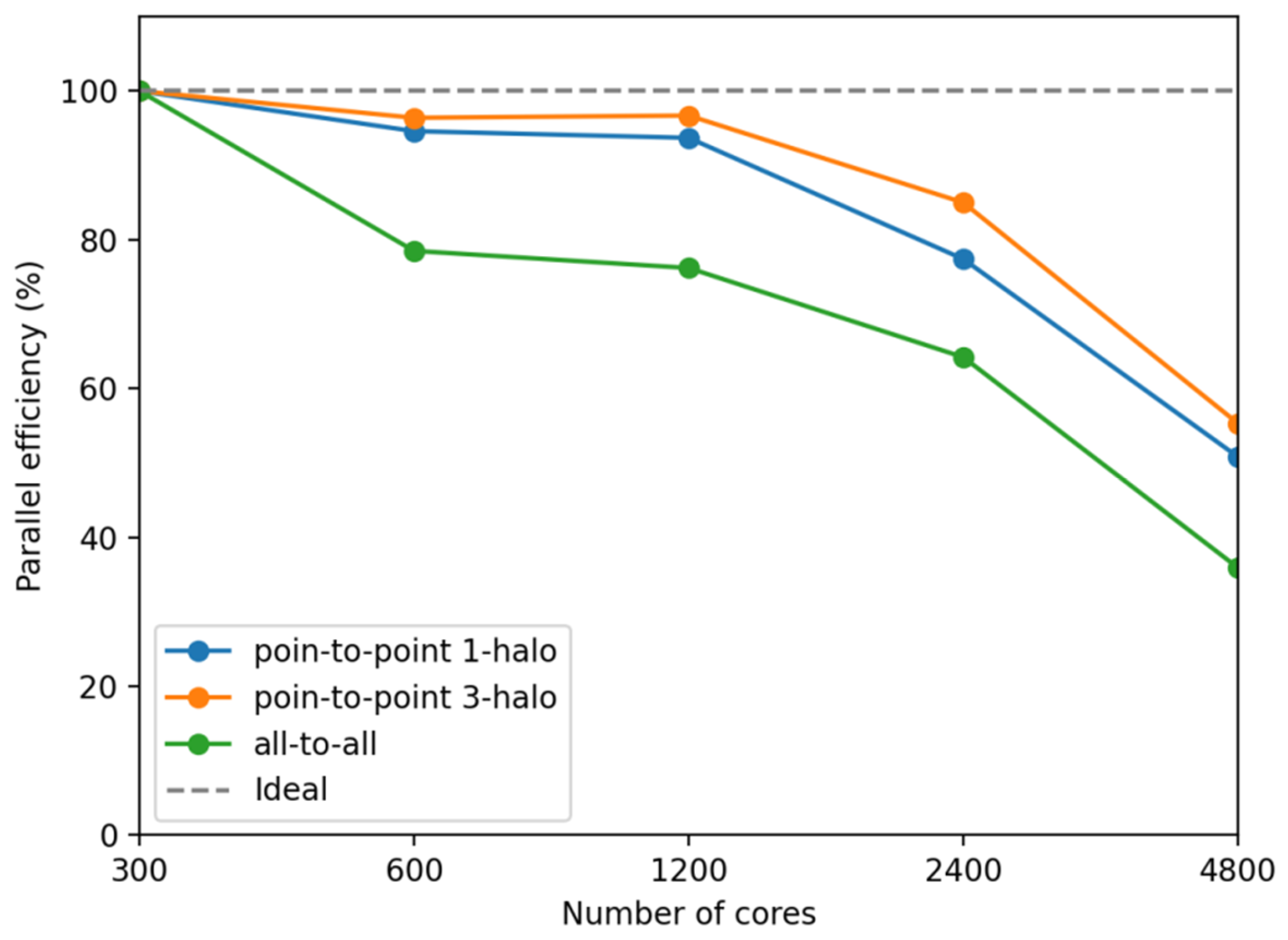
3.2.2. Parallel Efficiency of the Main Communication Patterns

The parallel efficiency of a model is the ratio between the acceleration of the code and the expected speedup. Concerning the presented code, the two point-to-point and one all-to-all communication operations scale at different rates and determine the parallel efficiency of the whole code. Figure 7 shows the parallel efficiency of these three operations for different configurations ranging from 300 CPU cores up to 4800 CPU cores for the waves propagating over the submerged elliptical shoal using a mesh of 800 × 256 × 240 cells. The scalability tests were performed at the MareNostrum4 supercomputer, where each node consists of two Intel Xeon Platinum 8160 of 24 CPU cores. Each MPI process was linked with 12 CPU cores, so 4 MPIs processes ran at each computer node. The acceleration of the code is calculated with respect to the setup using 300 CPU cores. Using three layers of halo cells attains a slightly better parallel efficiency than working only with one for the point-to-point communications. This occurs because the communication process involves gather and scatter operations before actually communicating the halo information. These operations accelerated a bit faster when the quantity of data is more significant. Moreover, part of the high network latency is hidden due to messages with more length. Even though the three-halo point-to-point communication has a better scaling, it still runs on average 44% slower than the one halo point-to-point communication.
On the other hand, the parallel efficiency of the all-to-all communication is the worst. The reason is that this communication pattern involves all the MPI processes with short messages (only 8 bytes). However, the all-to-all operation runs up to 6.7 times faster than the rest. The optimal number of cores for this test case is between 600 and 1200, achieving a parallel efficiency of 80% in all operations.

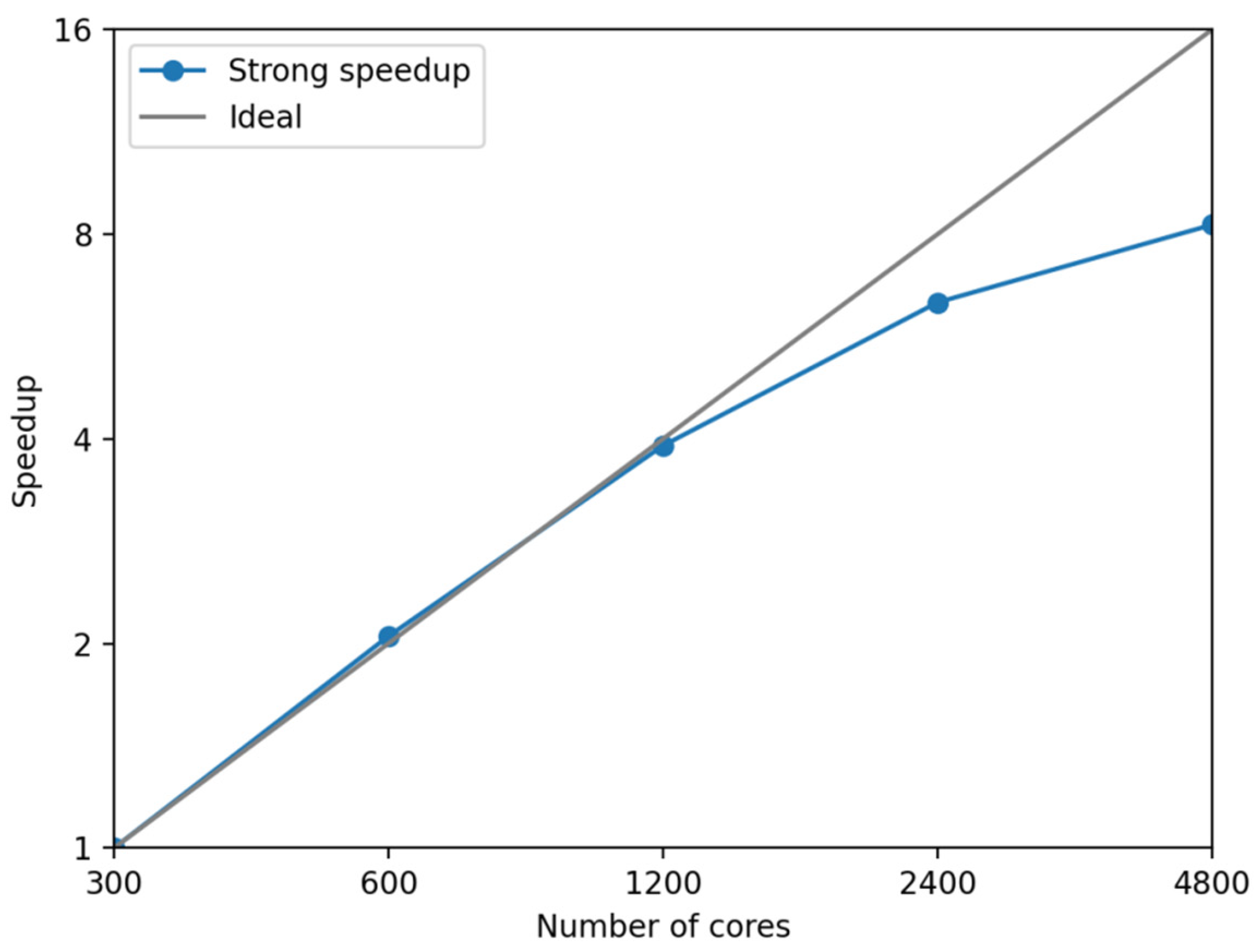
3.2.3. Strong Scaling of the Presented Code

The strong scaling of a numerical model is obtained by maintaining a constant problem size while increasing the number of computing resources utilized for its solution. Figure 8 depicts the strong scaling of the present simulation of propagating waves over a submerged elliptical shoal on a mesh of 800 × 256 × 240 cells. The scaling reference (300 CPU cores) was the minimal configuration in which the simulation runs due to memory demands. The presented code has a nearly linear scaling when using up to 1200 CPU cores. Keep in mind that the scaling of the code depends mainly on the linear solver (98%) that is composed of communications patterns of point-to-point of one halo and all-to-all. The acceleration of the code agrees with the individual analysis of those communications patterns. With up to 2400 CPU cores, the model is still within the range of a good scaling, with a parallel efficiency of 79%. Utilizing more CPU cores is not considered optimal since its parallel efficiency decreases to 51% (4800 CPU cores). Understanding the parallel behavior of the application is essential to use the computing resources efficiently.

4. Discussion and Concluding Remarks

An advanced numerical model was presented for the simulation of wave propagation over a submerged elliptical shoal, utilizing an efficient hybrid parallel implementation. The Navier–Stokes equations were solved using the LES approach. The 3D IB method was utilized for the enforcement of the no-slip boundary condition on the bed surface, whereas the tracking of the free-surface evolution was accomplished by the level-set method. The model was validated against experimental measurements and the combined wave refraction and diffraction patterns were accurately reproduced. Other than the wave transformation, the hybrid parallel implementation of the model produced depth-resolved flow results that the BTM or depth-averaged non-hydrostatic models cannot offer. In particular, the 3D flow in the vicinity of the shoal was simulated and the corresponding velocity and vorticity fields were presented. Finally, it was found that the optimal number of cores, for the simulation of cases C1 and C2, was 1200, achieving a parallel efficiency of 80% and an almost linear scaling.

Author Contributions

Conceptualization, G.A.L., I.A.C., and A.A.D.; methodology, G.A.L., I.A.C., G.O., and A.A.D.; software, G.A.L., I.A.C., and G.O.; validation, G.A.L., I.A.C., and G.O.; formal analysis, G.A.L., I.A.C., G.O., and A.A.D.; writing—original draft preparation, G.A.L., I.A.C., G.O., and A.A.D.; writing—review and editing, G.A.L., I.A.C., G.O., and A.A.D.; visualization, G.A.L., I.A.C., and G.O.; supervision, A.A.D.; project administration, G.A.L.; funding acquisition, G.A.L. All authors have read and agreed to the published version of the manuscript.

Funding

The present research has been co-financed by Greece and the European Union (European Social Fund—ESF) through the Operational Program “Human Resources Development, Education and Lifelong Learning”, in the framework of the “Supporting Postdoctoral Researchers-B cycle” (MIS 5033021) implemented by the State Scholarships Foundation (IKY).

Institutional Review Board Statement

Not applicable.

Informed Consent Statement

Not applicable.

Data Availability Statement

All numerical data are available, please contact by e-mail [email protected].

Acknowledgments

This work was supported by computational time granted from the National Infrastructures for Research and Technology S.A. (GRNET) in the National HPC facility-ARIS-under project ID pr009011_thin–CoastHPC.

Conflicts of Interest

The authors declare no conflict of interest.

References

  1. Karambas, T.V.; Memos, C.D. Boussinesq model for weakly nonlinear fully dispersive water waves. J. Waterw. Port Coast. Ocean Eng. 2009, 135, 187–199. [Google Scholar] [CrossRef]
  2. Shi, F.; Kirby, J.T.; Harris, J.C.; Geiman, J.D.; Grilli, S.T. A high-order adaptive time-stepping TVD solver for Boussinesq modeling of breaking waves and coastal inundation. Ocean Model. 2012, 43–44, 36–51. [Google Scholar] [CrossRef]
  3. Kirby, J.T. Boussinesq models and their application to coastal processes across a wide range of scales. J. Waterw. Port Coast. Ocean Eng. 2016, 142, 03116005. [Google Scholar] [CrossRef]
  4. Zijlema, M.; Stelling, G.; Smit, P. SWASH: An operational public domain code for simulating wave fields and rapidly varied flows in coastal waters. Coast. Eng. 2011, 58, 992–1012. [Google Scholar] [CrossRef]
  5. Yamazaki, Y.; Cheung, K.F.; Kowalik, Z. Depth-integrated, non-hydrostatic model with grid nesting for tsunami generation, propagation, and run-up. Int. J. Numer. Methods Fluids 2011, 67, 2081–2107. [Google Scholar] [CrossRef]
  6. Bai, Y.; Cheung, K.F. Depth-integrated free-surface flow with a two-layer non-hydrostatic formulation. Int. J. Numer. Methods Fluids 2012, 69, 411–429. [Google Scholar] [CrossRef]
  7. Wei, Z.; Jia, Y. Simulation of nearshore wave processes by a depth-integrated non-hydrostatic finite element model. Coast. Eng. 2014, 83, 93–107. [Google Scholar] [CrossRef]
  8. Bai, Y.; Yamazaki, Y.; Cheung, K.F. Convergence of multilayer nonhydrostatic models in Relation to Boussinesq-type equations. J. Waterw. Port Coast. Ocean Eng. 2018, 144, 06018001. [Google Scholar] [CrossRef]
  9. Smagorinsky, J. General circulation experiments with the primitive equations I. The basic experiment. Mon. Weather Rev. 1963, 91, 99–165. [Google Scholar] [CrossRef]
  10. Önder, A.; Yuan, J. Turbulent dynamics of sinusoidal oscillatory flow over a wavy bottom. J. Fluid Mech. 2019, 858, 264–314. [Google Scholar] [CrossRef]
  11. Oyarzun, A.G.; Chalmoukis, I.A.; Leftheriotis, G.A.; Dimas, A.A. A GPU-based algorithm for efficient LES of high Reynolds number flows in heterogeneous CPU/GPU supercomputers. Appl. Math. Model. 2020, 85, 141–156. [Google Scholar] [CrossRef]
  12. Jin, C.; Coco, G.; Tinoco, R.O.; Ranjan, P.; San Juan, J.; Dutta, S.; Friedrich, H.; Gong, Z. Large eddy simulation of three-dimensional flow structures over wave-generated ripples. Earth Surf. Process. Landf. 2021, 1–13. [Google Scholar] [CrossRef]
  13. Frantzis, C.; Grigoriadis, D.G. An efficient method for two-fluid incompressible flows appropriate for the immersed boundary method. J. Comput. Phys. 2019, 376, 28–53. [Google Scholar] [CrossRef]
  14. De Vita, F.; De Lillo, F.; Verzicco, R.; Onorato, M. A fully Eulerian solver for the simulation of multiphase flows with solid bodies: Application to surface gravity waves. J. Comput. Phys. 2021, 438, 110355. [Google Scholar] [CrossRef]
  15. Dodd, M.S.; Ferrante, A. A fast pressure-correction method for incompressible two-fluid flows. J. Comput. Phys. 2014, 273, 416–434. [Google Scholar] [CrossRef]
  16. Dimas, A.A.; Chalmoukis, I.A. An adaptation of the immersed boundary method for turbulent flows over three-dimensional coastal/fluvial beds. Appl. Math. Model. 2020, 88, 905–915. [Google Scholar] [CrossRef]
  17. Sethian, J.A.; Smereka, P. Level set methods for fluid interfaces. Annu. Rev. Fluid Mech. 2003, 35, 341–372. [Google Scholar] [CrossRef] [Green Version]
  18. Dimas, A.A.; Koutrouveli, T.I. Wave height dissipation and undertow of spilling breakers over beach of varying slope. J. Waterw. Port Coast. Ocean Eng. 2019, 145, 04019016. [Google Scholar] [CrossRef]
  19. Jacobsen, N.G.; Fuhrman, R.; Fredsøe, J. A wave generation toolbox for the open-source CFD library: OpenFoam®. Int. J. Num. Methods Fluids 2012, 70, 1073–1088. [Google Scholar] [CrossRef]
  20. Koutrouveli, T.I.; Dimas, A.A. Wave and hydrodynamic processes in the vicinity of a rubble-mound, permeable, zero-freeboard breakwater. J. Mar. Sci. Eng. 2020, 8, 206. [Google Scholar] [CrossRef] [Green Version]
  21. Oyarzun, G.; Borrell, R.; Gorobets, A.; Lehmkuhl, O.; Oliva, A. Direct numerical simulation of incompressible flows on unstructured meshes using hybrid CPU/GPU supercomputers. Procedia Eng. 2013, 61, 87–93. [Google Scholar] [CrossRef] [Green Version]
  22. Borrell, R.; Dosimont, D.; Garcia-Gasulla, M.; Houzeaux, G.; Lehmkuhl, O.; Mehta, V.; Owen, H.; Vázquez, M.; Oyarzun, G. Heterogeneous CPU/GPU co-execution of CFD simulations on the POWER9 architecture: Application to airplane aerody-namics. Future Gener. Comput. Syst. 2020, 107, 31–48. [Google Scholar] [CrossRef]
  23. Briggs, M.J. Summary of WET Shoal Results, Memorandum for Records; Coastal Engineering Research Center, Waterways Experiment Station: Vicksburg, MS, USA, 1987. [Google Scholar]
  24. Vincent, L.; Briggs, M.J. Refraction—Diffraction of Irregular Waves over a Mound. J. Waterw. Port Coast. Ocean Eng. 1989, 115, 269–284. [Google Scholar] [CrossRef]
  25. Kang, L.; Guo, X. Depth-integrated, non-hydrostatic model using a new alternating direction implicit scheme. J. Hydr. Res. 2013, 51, 368–379. [Google Scholar] [CrossRef]
  26. Fang, Z.; Liu, Z.; Zou, Z. Efficient computation of coastal waves using a depth-integrated, non-hydrostatic model. Coast. Eng. 2015, 97, 21–36. [Google Scholar] [CrossRef]
  27. Vasarmidis, P.; Stratigaki, V.; Suzuki, T.; Zijlema, M.; Troch, P. On the accuracy of internal wave generation method in a non-hydrostatic wave model to generate and absorb dispersive and directional waves. Ocean Eng. 2021, 219, 108303. [Google Scholar] [CrossRef]
  28. Viviano, A.; Musumeci, R.E.; Foti, E. A nonlinear rotational, quasi-2DH, numerical model for spilling wave propagation. Appl. Math. Model. 2015, 39, 1099–1118. [Google Scholar] [CrossRef]
  29. Ha, T.; Lin, P.; Cho, Y.S. Generation of 3D regular and irregular waves using Navier-Stokes equations model with an internal wave maker. Coast. Eng. 2013, 76, 55–67. [Google Scholar] [CrossRef]
  30. Raoult, C.; Benoit, M.; Yatesa, M.L. Development and validation of a 3D RBF-spectral model for coastal wave simulation. J. Comp. Phys. 2019, 378, 278–302. [Google Scholar] [CrossRef]
  31. Berkhoff, J.C.W.; Booy, N.; Radder, A.C. Verification of numerical wave propagation models for simple harmonic linear water waves. Coast. Eng. 1982, 6, 255–279. [Google Scholar] [CrossRef]
  32. Choi, J.; Lim, C.H.; Lee, J.I.; Yoon, S.B. Evolution of waves and currents over a submerged laboratory shoal. Coast. Eng. 2009, 56, 297–312. [Google Scholar] [CrossRef]
Figure 1. Example of one halo layer (left) and three halo layers (right) for a 6 × 6 2D subdomain.
Fluids 06 00350 g001
Figure 2. The computational domain used for the numerical simulation of wave propagation over an elliptical shoal. Planes T1–T4 indicate the position of the measurement transects that were used for the numerical model validation.
Fluids 06 00350 g002
Figure 3. (a) Instantaneous free-surface snapshot, after the propagation of 10 waves over the submerged elliptical shoal, for case C2. The computational domain with the Cartesian grid is shown every 4th node. The ratio of the horizontal axes scale to the vertical one is 0.2; (b) the corresponding spanwise velocity contours on the free surface over and downstream of the shoal.
Fluids 06 00350 g003
Figure 4. Instantaneous flow field, at the cross section of the domain centerline, for case C2: velocity (vectors) and spanwise vorticity, ωy, (contours). The ratio of the horizontal axis scale to the vertical one is 0.2.
Fluids 06 00350 g004
Figure 5. Comparison between present numerical results (red lines), experimental measurements (black squares), and numerical results in the literature (blue line and black dashed line) for the normalized wave height H/H0, along the four transects shown in Figure 2, for case C1.
Fluids 06 00350 g005
Figure 6. Comparison between numerical results (red lines) and experimental measurements (black squares), for the normalized wave height H/H0, along the four transects shown in Figure 2, for case C2.
Fluids 06 00350 g006
Figure 7. Parallel efficiency of the three main communication patterns of the presented code on a computational mesh of 800 × 256 × 240 cells.
Fluids 06 00350 g007
Figure 8. Strong speedup of the presented code on a computational mesh of 800 × 256 × 240 cells.
Fluids 06 00350 g008
Table 1. The main stages of the algorithm.
1.Computation of the intermediate velocity field;
2.Implementation of the IB method (no-slip condition);
3.Computation of the pressure field—Equation (4);
4.Computation of the final velocity field—Equation (3);
5.Computation of the evolution of the free surface—Equation (5).
Table 2. Incident wave characteristics of the two simulated cases.
Test CaseWave Height,
H0 (cm)
Wave Period,
T (s)
C15.501.3
C27.751.3
Table 3. RMSE (%) of the present numerical results with respect to the experimental measurements in Vincent and Briggs [24] and Briggs [23] for cases C1 and C2.
RMSE (%)Test Case C1Test Case C2
T19.766.73
T25.288.04
T37.4422.6
T49.4120.2
Table 4. Relative temporal weight of the main operations involved in the simulation of the wave propagating over the submerged elliptical shoal using 49.152 million cells.
Stage of the AlgorithmRelative Weight
1.Computation of the intermediate velocity field;0.73%
2.Implementation of the IB method (no-slip condition);0.37%
3.Computation of the pressure field—Equation (4);98.19%
4.Computation of the final velocity field—Equation (3);0.17%
5.Computation of the evolution of the free surface—Equation (5).0.54%
Publisher’s Note: MDPI stays neutral with regard to jurisdictional claims in published maps and institutional affiliations.

