Article

The Impacts of Gustiness on Air–Sea Momentum Flux

1
Department of Oceanography, Texas A&M University, College Station, TX 77843, USA
2
Coastal and Hydraulics Laboratory, U.S. Army Engineering Research and Development Center, Duck, NC 27949, USA
*
Author to whom correspondence should be addressed.
Fluids 2021, 6(10), 336; https://doi.org/10.3390/fluids6100336
Submission received: 1 May 2021 / Revised: 10 September 2021 / Accepted: 16 September 2021 / Published: 22 September 2021
(This article belongs to the Special Issue Boundary Layer Processes in Geophysical/Environmental Flows)

Abstract

:
The exchange of momentum across the air–sea boundary is an integral component of the earth system and its parametrization is essential for climate and weather models. This study focuses on the impact of gustiness on the momentum flux using three months of direct flux observations from a moored surface buoy. Gustiness, which quantifies the fluctuations of wind speed and direction, is shown to impact air–sea momentum fluxes. First, we put forward a new gustiness formula that simultaneously evaluates the impact of fluctuations in wind direction and speed. A critical threshold is established using a cumulative density function to classify runs as either gusty or non-gusty. We find that, during runs classified as gusty, the aerodynamic drag coefficient is increased up to 57% when compared to their non-gusty counterparts. This is caused by a correlated increase in vertical fluctuations during gusty conditions and explains variability in the drag coefficient for wind speeds up to 20 m/s. This increase in energy is connected with horizontal fluctuations through turbulent interactions between peaks in the turbulent spectra coincident with peaks in the wave spectra. We discus two potential mechanistic explanations. The results of this study will help improve the representation of gustiness in momentum flux parameterizations leading to more accurate ocean models.

1. Introduction

In the marine boundary layer, the ocean is tightly coupled to the atmosphere through the wind stress τ . The wind stress is a quantification of the momentum flux across the air–sea interface which is important for many processes such as wave growth and breaking [1,2,3], aerosol production [4], atmospheric and oceanic circulation (e.g., [5,6,7]), global climate [8], and upper ocean mixing (e.g., [9,10]). The momentum flux is also a key component of tropical cyclone intensity [11].
In the constant-flux layer the total wind stress can be decomposed into three parts:
τ = τ t + τ w + τ v    
Here, τ t is the turbulent stress, τ w the wave-induced stress, and τ v the viscous stress [12]. τ v is caused by the differential of wind and sea surface current speed within the viscous sub-layer which has a thickness on the order of 10 5 m, much thinner than the wave-induced boundary layer [12,13], and is negligible away from the sea surface. τ w occurs in the wave-boundary layer, within which air flow is influenced by waves [14]. The wave-boundary layer height has been shown to depend on wind speed [15,16] and sea state [17], and is predicted to be order 1 m for pure wind sea conditions in [18]. It has also been demonstrated that the wave induced stress is less than 5% of the total stress at the height of 1 m, and less than 1% at 3 m. Previous experiments have established the practice of making measurements 3–4 m above the sea surface e.g., [19,20] where viscous and wave-induced stress were deemed negligible. (i.e., τ τ t τ w τ v ). Under such conditions, turbulent fluxes approximate the total momentum flux, e.g., [21]:
τ t τ t = ρ u w ¯ ρ v w ¯        
Here u , v ,   and   w ,   are velocity in the along, cross, and downwind directions, respectively, with primes denoting the fluctuating component and overbar representing time average (O~30 min). Air–sea coupling within the marine boundary layer is widely parameterized by the wind stress equation:
τ = ρ u * 2 = ρ C d U 10 2        
where u * is the shear or friction velocity of the wind at the sea surface, ρ is the air density, C d is the drag coefficient, and U 10 is the wind speed at a reference height of 10 m. Combining Equations (2) and (3), we arrive at Cd, calculated from direct measurements
C d = ( u w ) ¯ 2 + ( v w ) ¯ 2 U 10 2         .
Because of the isolation and harsh environmental conditions, measuring fluxes at sea is very challenging and expensive, especially at high wind speeds. As such, it is common for the momentum flux to be determined instead by using the nondimensional drag coefficient as a function of the mean wind speed. Since the drag coefficient is widely adopted and used in lieu of direct flux measurements when quantifying air–sea momentum exchange (e.g., [22,23]), we focus on the impact of gustiness on the drag coefficient such that results have direct implications for Earth system models.
Many studies have shown that C d increases approximately linearly with wind speed [21,24,25]. However there remains substantial variability in C d . Several secondary variables have been shown to affect C d , including sea state [19,26,27,28,29], currents [6], air–sea temperature difference and stability [3,30], and gustiness [30,31].
Many studies have quantified the influence of sea state on C d . Results show that wave age C p / U 10 , where C p is the phase speed of the peak wave frequency, is well correlated to C d [24,27,32,33], and C d tends to be higher in young seas, C p / U 10 < 1.5 . The association between wave age and C d is not surprising given that young waves are steeper and rougher than old waves [29,34,35]. Also based on the association between wave age and drag, Oost et al. [36] found a reliable relationship between for C p and ocean roughness.
The impacts of swell on C d have also been extensively investigated with mixed results. For example, Dobson et al. [37] found no evidence that swell influences C d , but Drennan et al. [38] observed reduced wind stress in the presence of swell. This finding was supported by the finds of Potter [39], who determined that swell can reduce C d up to 37% due to the reduced turbulent energy around the swell frequency. In contrast, Drennan et al. [40] found that both crossing- and opposing-swell significantly increase C d , and Vincent et al. [41] showed an increase in drag due to increased energy in the high-frequency waves relative to pure wind seas, consistent with their previous work [42]. Increased drag coefficient in the left-rear of a tropical cyclone where conditions are thought to be predominantly crossing and opposing-swell, has also been shown [28].
Surface currents have been shown to reduce C d , especially when the current is aligned with the wind [30]. Kara, Metzger, and Bourassa [7] reported that C d can be reduced over 10% in the tropical Pacific Ocean due to currents being in line with the prevailing winds. Furthermore, a numerical modelling study of an idealized typhon showed that surface current can reduce the momentum fluxes in the right-rear typhoon quadrant about 6% in [5]. In contrast, Wüest and Lorke [43] found that currents in the Kuroshio Extension have very little influence on C d . Currents can also affect the momentum fluxes in indirectly; Kenyon and Sheres [44] found that strong current gradients impact the surface gravity wave field which can then affect air–sea momentum fluxes.
The stability of atmosphere influences C d according to Monin–Obukhov similarity theory [45,46,47,48,49]. Monin and Obukhov [50] put forward the Obukhov length to describe the air–sea fluxes processes.
L = v * 3 k ( g T 0 ) ( q C t ρ )          
where k is the von Karman constant, T 0 is surface temperature, g is gravity acceleration, v * is friction velocity, q is kinematic heat flux, C t is specific heat, and ρ is air density. The Obukhov length accounts for the relationship between sea surface temperature, specific heat, air density, heat flux, and friction velocity. In light winds, the momentum fluxes are sensitive to the stability of the atmosphere, with increased flux for unstable conditions [51].
While much attention has been given to sea state, currents, and atmospheric stability, there are few studies that directly address the effect of gustiness on C d . The importance of accounting for gustiness when estimating momentum fluxes was first addressed by Janssen [52], who believed that the friction velocity should be related to both the mean and standard deviation of wind speed. Miles and Ierley [53], using a theoretical model, found that, under some circumstances, 20–30% more energy is transferred to the ocean during gusty conditions but that a reduction in the stress is also possible. Abdalla and Cavaleri [54] used a model to compare the wave field under normal and gusty winds and found that wave height is increased under gusty conditions, implying increased momentum flux. Ponce and Ocampo–Torres [55] also showed that wind speed variability increases wave height while Pleskachevsky et al. [56] remotely observed higher wave height under the influences of gustiness. Annenkov and Shrira [57] studied wave responses to different gustiness regimes using an idealized numerical model. They found that gustiness can impact growth rate during wave development but had little impact as waves approached full development. Uz et al. [58] found that decreasing winds had higher wind stress than the increasing winds for any given wind speed, which is mainly caused by the delayed response of short wind waves to the modulated wind forcing.
Previous research notwithstanding, it is very difficult to account for the impact of gustiness on momentum flux because typical wind speed data, whether extracted from satellite remote sensing, collected in situ, or model derived, are produced as an average over space and/or time and so high frequency fluctuations are unknown. As such, it is difficult to incorporate gustiness information into C d parameterizations. Babanin and Makin [31] addressed this by developing a method to estimate maximum gustiness using U 10 , which can be then used to estimate the contribution of gustiness to C d for any given wind speed. In their study, gustiness was quantified using the mean and standard deviation of wind speed calculated over 30 min:
G = s t d ( U 10 ) / U 10 ¯                        
Following Babanin and Makin [59], Ting et al. [60] found that gustiness can increase scatter in C d , and used a scale analysis based on the equation of motion to determine that wind stress was proportional to gustiness. They speculated that the variability in the drag coefficient was caused by gustiness through distortion of the air–sea boundary layer structure. The Coupled Ocean-Atmosphere Response Experiment (COARE) algorithm [30] represents gustiness as boundary layer–scale eddies and is more akin to vertical thermal stability rather than horizontal wind fluctuations.
In this study, we focus on the influence of gustiness on the momentum flux. We introduce a gustiness formula that is sensitive to the fluctuations of both wind speed and direction. The metric captures variation within scales of 0.01–1 Hz. We apply the new formula to data from the Impact of Typhoons on the Ocean in the Pacific (ITOP) experiment [61]. Our results indicate that gusty periods exhibit higher C d than predicted by the linear wind speed parameterization [25]. We also used a scaled Miyake-Cospectrum [62] to explore the momentum fluxes transferred into the ocean. This Miyake-Cospectrum is normalized by wind speed, which is helpful for comparing the gustiness influences under different mean wind speeds. We ultimately conclude that gustiness is important to C d , accounting for about 57% of the variability in C d . We also find that the cospectra of the momentum flux is proportional to the gustiness. When winds are gusty, we find an associated increase in energy in the cospectra.

2. Data and Methods

2.1. Data

Data used in this study were collected during the Impact of Typhoons on the Ocean in the Pacific (ITOP) experiment [61]. Data were collected between August and December 2010, from an instrumented Extreme Air–Sea Interaction (EASI) buoy (Drennan et al. [63]) deployed in the Philippine Sea approximately 750 km east of Taiwan. Direct fluxes were measured onboard with simultaneous mean parameters including air and ocean temperature, humidity, and atmospheric pressure. The EASI buoy, which was based on the hull of a 6-m Navy Oceanographic Meteorological Automatic Device (NOMAD), also measured directional wave spectra that were produced over 30 min, as was wind speed [64]. Several studies have previously used data collected by EASI during ITOP (e.g., [9,27,39,63,65]) and provide extensive information about the experiment, instrumentation, and data processing and quality. Here, we only reproduce information about the wind sensors and associated processing methods.
The EASI buoy was equipped with two Gill R2A sonic anemometers. However, due to severe weather, only one R2A anemometer collected reliable data. The sampling frequency of the wind anemometer was 20 Hz with runs of 30 min, which was found suitable for collecting all turbulent scales [66]. The anemometer was positioned 5.45 m above mean sea level and away from the buoy structure such that flow distortion was negligible. Two motion packages in the buoy measured six degrees of freedom of motion along with the compass bearing. The motion of the platform was accounted for when calculating the wind velocity in accordance with the methods by [67]. Following motion-correction, a quality control procedure removed spikes in the 20 Hz u , v , and w time series [66]. Ogives were calculated and it was revealed that the scales of 0.01–1.0 Hz were adequate to fully characterize momentum flux, as expected from universal curves [62]. Next, u , v , and w were rotated according to the mean wind vector so that the w was around 0 and u pointed towards the mean wind direction, thereby m e a n ( v ) = 0 . These data were then used to calculate C d following Equation 4. Log layer theory was used to adjust the value of C d to the equivalent measured at 10 m in neutral conditions, which is referred to as C d 10 N .

2.2. Gustiness Formulation
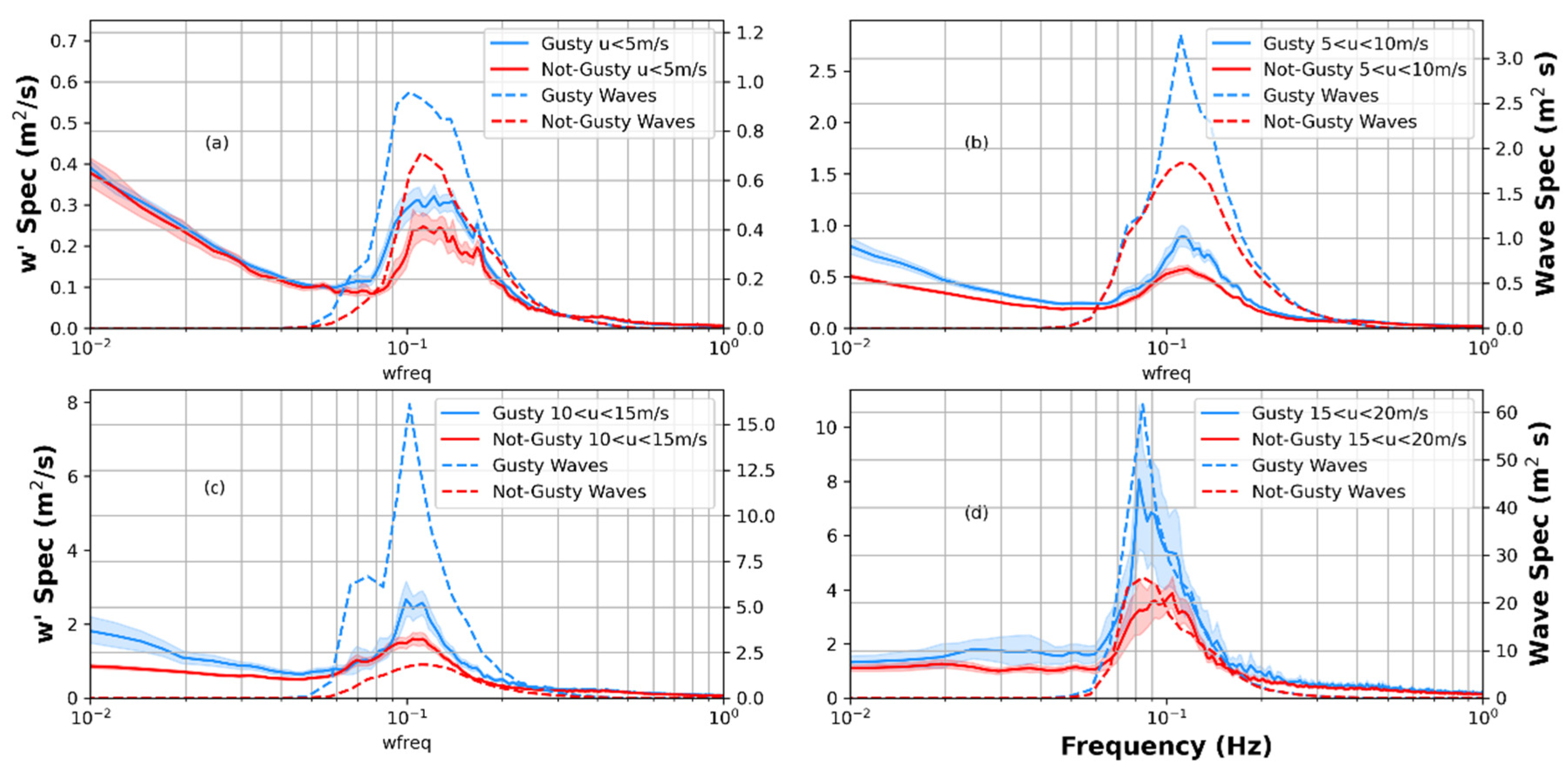
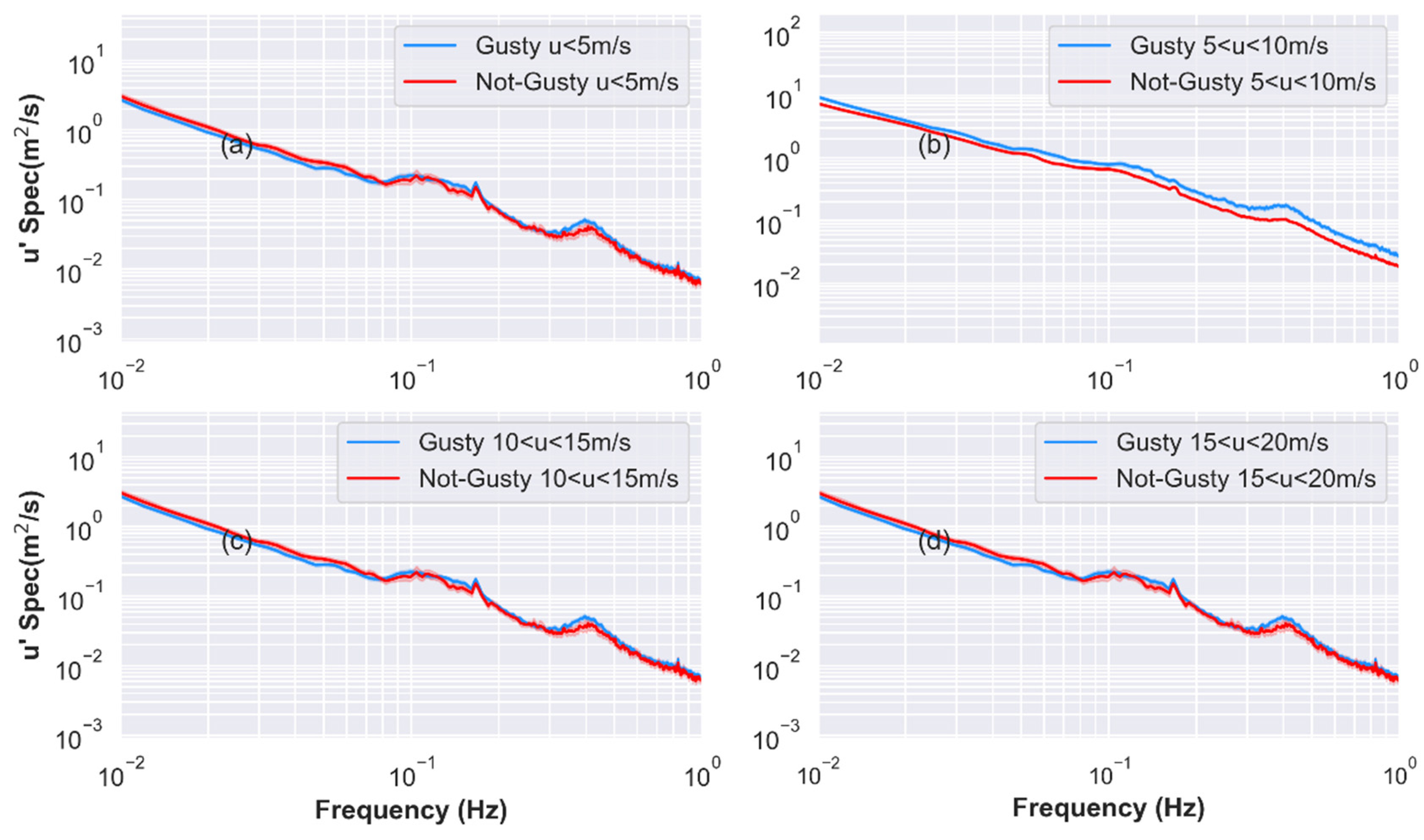
The Babanin and Makin [31] equation for gustiness (Equation (5)) quantifies the fluctuation of wind speed but does not consider wind direction variability. We show that directional variability can also increase variance in both u and v , and therefore must be part of the gustiness formulation in order to more fully characterize wind variability. For example, if wind speed is constant, the runs with unstable direction will contain more turbulent energy than runs with stable direction. As such, we put forward a new gustiness formula, G A , (Equation (7)), to account for fluctuations in both wind speed and direction.
G A = s t d ( u + v ) / U 10                  
Equation (7) can be expanded as below:
s t d ( u + v ) / U 10 = v a r ( u ) + v a r ( v ) + 2 c o v ( u , v ) / U 10
The c o v ( u , v ) term represents the influence of changing wind direction, and it reduces to 0 when the wind direction is stable. Supposing at one moment that the mean wind direction has turned about x degrees, it will add an extra fluctuation ( u , v ) ~   U · ( 1 c o s x , s i n x ) to the original wind vector. A change in wind direction projects an extra velocity onto the ( u , v ) . It can be seen that the added fluctuation ( U U c o s x , U s i n x ) is correlated, which is one source of the covariance term. One thing to note, c o v ( u , v ) can be underestimated to some extent given that some portions of ( u , v ) are still independent, similar to Brownian motion [68], when the wind direction is changing. When c o v ( u , v ) 0 , observation samples of ( u , v ) are distributed symmetrically but the main axis is not along the x or y axis. Graphical representations of c o v ( u , v ) = 0 and c o v ( u , v ) 0 are shown in Figure 1.
To better characterize G A , sensitivity to sampling frequency was explored. Figure 2 shows the standard deviation of u + v for an arbitrary run as a function of sampling frequency. When the frequency reaches approximately 1 Hz, s t d ( u + v ) converges upon a constant value, in this case 1.83. This is a typical result (though other runs converge upon different values), indicating that our sampling frequency of 20 Hz is more than adequate to obtain a stable standard deviation of u   and   v .
Our definition of gustiness is sensitive to run length because of the increased potential for wind direction change with time. Thirty-minute run-time is a compromise between a length adequate to capture all turbulent length scales (e.g., [19,37,63]) and short enough such that stationarity is not violated. This record length was used in many previous studies focused on Cd (e.g., [19,21,24,38,66,69]), and, furthermore, 30 min is a typical time domain used by air–sea coupled climate or hurricane models (e.g., [70,71]). Hence, by adopting a 30 min sampling period, we seek to maximize the applicability of the results to future research.

3. Results

Figure 3 shows the times series of wind speed ( U 10 N ) and gustiness G A . High G A can be attributed to the fluctuation of wind speed and direction or low U 10 N , which increases G A in Equation (7).
Figure 4 shows the cumulative probability function of G A for all the runs to help define a limit above which the wind is gusty. G A of gusty and not-gusty runs is calculated via Equation (6). A value of 0.165 was chosen for selecting gusty runs and represents the time when the CPF is 50%.
Based on the formula for G A , Figure 5 shows C d 10 N as a function of U 10 N . Each data point is color coded by gustiness, with dark green indicating G A     0.165 . When the winds are not gusty, a clear linear relationship between C d 10 N   &   U 10 N emerges. This relationship is similar to the linear empirical equation proposed by [25,30]. This suggests that these widely used linear equations were established based on data collected during relatively wind speed stable conditions. Most gusty points are over this linear relationship, suggesting that gusty conditions are generally associated with an increase in momentum flux. From the error bar plot, for moderate winds (5–12 m/s), we find that the variation in C d 10 N of winds can be reduced by as much as 57% by removing the gusty runs.
Figure 6 shows C d 10 N vs. U 10 N . Points are colored by the covariance term,   | c o v ( u , v ) | / U 10 . This term can be attributed to the changing wind direction, since a change in direction ( θ ) will add extra correlated oscillation u ~ U 10 · ( 1 c o s θ ) ,   v ~ U 10 · s i n θ to the fluctuation. The covariance term will be increased when the direction is turning. Therefore, Figure 6 indicates that changing wind direction could play an important role in contributing to the gustiness, and thus C d . In another words, some scatter in C d , or increased gustiness, can be explained by changes in direction. To parallel this viewpoint, the data are plotted again (Figure 7), but are now identified based on the stability of their wind speed and direction. Here, we used s t d ( u ) > 1 m / s and s t d ( θ ) > 7 ° to identify runs that were considered either wind speed unstable or wind direction unstable. Using these values results in 25% and 31% of data characterized as gusty due to variability in speed and direction, respectively. For comparison, if we set the threshold to 0.5, 2, or 3 m/s, the percentage of gusty data would be 78%, 4%, 0.7%, respectively. Setting the threshold to 3, 5, or 10° would result in 100%, 82%, and 11%, respectively, classed as gusty. Most importantly, Figure 7 shows that deviations in both speed and direction are important considerations when quantifying gustiness. Notably, directional deviations identify much of the scatter in the U 10 N C d 10 N relationship at low to moderate wind speeds that cannot be captured when considering fluctuations in wind speed alone. Furthermore, we avoid another issue with identifying gustiness based on wind speed, which is that all data above ~15 m s−1 are classified as gusty because, inherently, s t d ( u ) increases with U .
We find that variations in both wind speed and direction can have significant influences on C d . In fact, the stability of wind direction is potentially a better metric than the stability of wind speed (Figure 7). When wind direction is stable, a linear relationship suggested by previous studies (e.g., [21,24,66]) between C d 10 N and U 10 N emerges. In contrast to c o v ( u , v ) , speed stability does not correlate with variation in C d 10 N   at moderate wind speeds (5–12 m/s). This implies that direction is more effective in explaining the variation in C d 10 N .

4. Discussion

4.1. Gustiness and Vertical Oscillation

Next, we examine in detail the difference between a gusty run and a not-gusty run. Figure 8 shows a histogram of the distribution of u &   v over 30 min for two different runs. These runs are controlled for wind speed, i.e., both have U 10 N = 10   m / s . For Figure 8a, G A = 0.12 (low gustiness), and for Figure 8b, G A = 0.21 (high gustiness). In each panel there are 36,000 data points (i.e., 30 min * 60 s * 20 Hz) of ( u , v ) that distribute around (0,0) in a cloud of points. In Figure 8a, the data are distributed symmetrically, forming a circle, and the histogram is symmetric, which indicates the wind direction remained relatively stable. In Figure 8b, the data are asymmetrically distributed over a larger area in u , v space, skewed towards the lower-left. In this case, the distribution is an ellipse and the major axis is rotated away from the wind direction, indicating that the direction was changing over the duration of the run. In Figure 8c, the directions of the gusty and non-gusty runs are shown. We can see that the direction of the run in Figure 8b has changed about 20 degrees over 30 min, while the direction of the not-gusty run in Figure 8a has a negligible trend.
Note that the mean of | w | in Figure 8a,b is larger during the gusty run than the non-gusty. This suggests a stronger vertical oscillation in the gusty runs which may account for the observed higher C d . To explore this further, we plot the mean of | w | in Figure 9 as a function of wind speed for all our data. This shows that gusty periods tend to have higher | w | compared to periods when the wind speed and direction remain more stable, as determined using G A = 0.165 . This indicates a stronger oscillation in the vertical direction during gusty conditions which, when correlated with the u , v , increases C d . For moderate winds speeds, | w | is 30~50% larger for gusty than non-gusty periods. Hence, higher gustiness can inspire a stronger vertical oscillation, which transports the extra energy across the air–sea interface.
We now offer two potential explanations for the source c o v ( u , v ) term. The first source is that the wind direction is changing while the other is that the waves may be intermittently coupling with the gustiness. When the wind stress is between wave and wind directions, waves can explain some gustiness. These two sources may function simultaneously. We inspected many cases finding that, for a few runs, the stress direction was in between the wave direction and wind direction.

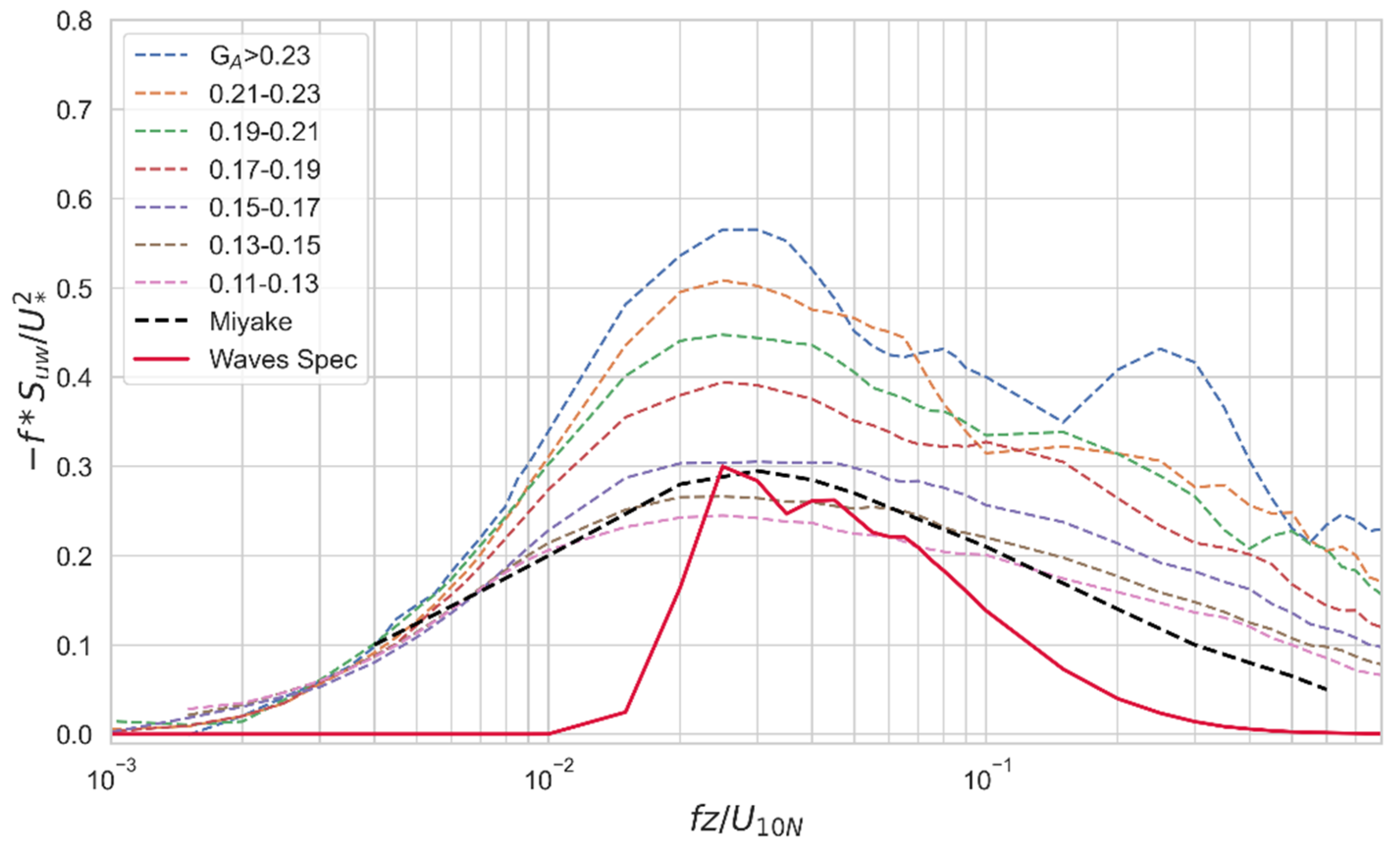
4.2. Possible Reason and Evidence for the Increased Momentum Fluxes

Figure 10 shows the mean power spectra of w for the entire data set. Each subplot represents a different wind speed range, data are further subdivided based on gusty and non-gusty conditions. Concurrent mean wave spectra are overlaid on the turbulence spectra. Turbulent power spectra can be seen to increase with wind speed, as expected; however, in each case, the gusty conditions are always more energetic than the non-gusty runs. For the lowest wind speeds, the gusty case has 20% higher energy, increasing to over 50% at the highest wind speeds. The increases are concentrated around the peak frequency. The peak frequencies of the wave spectra are located around the peaks in the w spectra, which shows some coupled or at least correlated behavior between turbulence and waves. This is true whether or not conditions are gusty. This analysis is repeated for u spectra (Figure 11) and no difference is found between the u power spectrum of gusty and not-gusty runs (p < 0.05). The same is true of v (not shown), i.e., there is no marked increase in energy in horizontal velocity at ocean wave scales. This suggests that the increased C d during gusty conditions is due to increased energy in the vertical oscillation.
Figure 10 shows that gusty runs coincided with more energetic w spectra. When more energetic w is correlated with u , gustiness translates directly to increased momentum flux. Figure 11 shows the u spectra, in which there are less changes in the spectra. To investigate whether this extra energy is correlated with u , we examine a probability density function (PDF) of normalized momentum flux in Figure 12. The momentum flux is normalized by friction velocity ( u w / u * 2 ) where u * 2 is estimated using [25] and the data are binned by G A . Positive values represent momentum transferred into the ocean and negative values are momentum transferred into the atmosphere. The PDFs have asymmetric shapes skewed towards positive values. This means downward momentum fluxes exceed the upward fluxes. As G A increases, the PDFs flatten and the probability of high and low u w / u * 2 increases, while the probability of u w / u * 2 around zero decreases. This shows that more energetic w do indeed increase momentum flux to the ocean.
To show how much the net momentum fluxes increased as a result of gustiness, we introduce the u w dimensionless cospectrum, which is scaled using the Miyake formula [62]. This spectrum can contain valuable information about momentum fluxes [30,38,72]. To quantify the net momentum flux, we integrate the u w cospectra along the frequency domain.
u w ¯ = 0 S u w d f
Here, S u w is the real part of the cross spectrum of u   and   w . Figure 13 exhibits the cospectra scaled by mean wind speed U , the measurement height z , and u * . Cospectra are shown for different gusty conditions along with the Miyake universal curve, which is widely used in similar studies [38,39,41].
In Figure 13, the magnitude of each spectrum increases with increasing gustiness. The cospectra therefore present further evidence that gustier winds have higher momentum fluxes. The energy containing region of the wave spectrum is aligned with that of the cospectra. This overlapping of energetic scales suggests some connection or coupling between the surface waves and the winds. The energy of the vertical turbulence spectra is strengthened in the presence of high gustiness. Although gustiness is characterized by horizontal wind variance, it is clear that when it is gusty there is a coincident increase in the vertical wind variance and at a similar turbulent scale-around 0.10 Hz. The vertical wind variance is connected with the horizontal wind variance due to the turbulent interactions and cascade of energy, which is isotropic. We know that, close to the sea surface, some of the vertical wind variance is coherent with the surface waves, however, direct physical connection remains unclear.
Among the possible explanations, we propose two potential mechanisms for how gustiness can cause the stronger w . First, when the wind direction is rotating, it will cause extra horizontal turbulence and produce additional positive vorticity in the z -direction. Additionally, the ocean surface has a frictional force which can consume this vorticity, which is to say a negative vorticity in the z -direction induced by friction. For example, in a cylinder, extra positive vorticity in the upper layer will be balanced by the negative vorticity held in the bottom layer. In this case, this mechanism causes friction upon the sea surface and may explain the increased w during gusty conditions. Another potential mechanism is that, when the wind speed is increasing, the vertical shear will be strengthened, in turn inspiring a lateral vorticity. For example, when U is increasing, it can create a positive vorticity in the mean wind direction. The only way to consume this extra vorticity is by bottom friction. In this case, small-scale lateral circulation will be produced which can connect the bottom wave surface layer with the upper layer. Ultimately, stronger vertical mixing occurs. However, proof of these two potential mechanisms requires more detailed observations to understand energy pathways and how the extra vorticity is balanced. For example, it is advisable to use the Particle Image Velocity method to take snapshots of the vertical profiles of the winds near the air–sea interface in a laboratory water tank or over the ocean. Measurements made at multiple levels may also help to understand the processes when the gustiness becomes increased.

5. Summary and Conclusions

A new gustiness formula [Equation (8)] is put forward which quantifies the fluctuations of wind speed and direction. We find that it is important to account for wind direction in explaining variability in the drag coefficient. We find that gustiness can increase C d independent of mean wind speed. The nominal linear relationship between C d and U 10 put forward by previous studies (e.g., [19,24,30], etc.) is found to emerge under non-gusty (or less gusty) conditions. From examining spectra, more energetic vertical turbulence is correlated with gustiness and is perhaps induced by some of the same mechanisms that produce gustiness. The wind cospectra and wave spectra share a peak frequency, suggesting a coupling between the two. From investigation of the cospectra and PDFs, the gusty winds have a clear increase in the normalized momentum fluxes, proving that gustiness results in extra momentum flux under the same wind speed. Overall, gustiness is an important factor for understanding momentum fluxes into the ocean and should be considered in an effective parameterization.

Author Contributions

Conceptualization, M.L. and H.P; methodology, M.L. and H.P.; software, M.L.; validation, M.L.; formal analysis, M.L., H.P. and C.O.C.; investigation, M.L.; resources, H.P. and C.O.C.; data curation, M.L., H.P. and C.O.C.; writing—original draft preparation, M.L.; writing—editing, H.P. and C.O.C.; visualization, M.L.; supervision, H.P. All authors have read and agreed to the published version of the manuscript.

Funding

ITOP was funded by the Office of Naval Research under Grant N0014-09-1-0392 with additional support from the National Science Foundation under Grant OCE-0526442.

Data Availability Statement

ITOP data are freely available from EOL data archives at https://data.eol.ucar.edu/ (accessed on 1 January 2019).

Acknowledgments

We would like to acknowledge and thank many people at the University of Miami who were involved in collection of the data we used here, especially Hans Graber and William Drennan, and their team, Neil Williams, Mike Rebozo, Rafael Ramos, and many graduate students. We are also thankful to the Woods Hole Oceanographic Institution mooring team, Environment Canada, and the Captain and Crew of the R/V Roger Revelle who contributed to the project success. COC was supported by the USACE civil works under the CODS program managed by Spicer Bak. We thank the Chinese Scholarship Council who helps support Meng Lyu’s graduate studies. Finally, we thank the five anonymous reviewers and the editors.

Conflicts of Interest

The authors declare no conflict of interest.

References

  1. Miles, J.W. On the generation of surface waves by shear flows. J. Fluid Mech. 1957, 3, 185–204. [Google Scholar] [CrossRef]
  2. Melville, W.; Romero, L.; Kleiss, J.; Swift, R. Extreme wave events in the Gulf of Tehuantepec. In Proceedings of the Rogue Waves: Proceedings 14th ‘Aha Huliko ‘a Hawaiian Winter Workshop, Manoa, HI, USA, 24–28 January 2005; pp. 23–28. [Google Scholar]
  3. Young, I.R.; Banner, M.L.; Donelan, M.A.; McCormick, C.; Babanin, A.V.; Melville, W.K.; Veron, F. An integrated system for the study of wind-wave source terms in finite-depth water. J. Atmos. Ocean. Technol. 2005, 22, 814–831. [Google Scholar] [CrossRef]
  4. Zavarsky, A.; Booge, D.; Fiehn, A.; Krüger, K.; Atlas, E.; Marandino, C. The influence of air-sea fluxes on atmospheric aerosols during the summer monsoon over the tropical Indian Ocean. Geophys. Res. Lett. 2018, 45, 418–426. [Google Scholar] [CrossRef] [Green Version]
  5. Fan, Y.; Ginis, I.; Hara, T. The effect of wind–wave–current interaction on air–sea momentum fluxes and ocean response in tropical cyclones. J. Phys. Oceanogr. 2009, 39, 1019–1034. [Google Scholar] [CrossRef] [Green Version]
  6. Kara, A.B.; Metzger, E.J.; Bourassa, M.A. Ocean current and wave effects on wind stress drag coefficient over the global ocean. Geophys. Res. Lett. 2007, 34, L01604. [Google Scholar] [CrossRef]
  7. Kara, B.; Metzger, J.; Bourassa, M. Impacts of Ocean Currents and Waves on the Wind Stress Drag Coefficient: Relevance to Hycom; Naval Research Lab Stennis Detachment Stennis Space Center MS: Stennis Space Center, Kiln, MS, USA, 2006. [Google Scholar]
  8. Roberts, M.J.; Camp, J.; Seddon, J.; Vidale, P.L.; Hodges, K.; Vannière, B.; Mecking, J.; Haarsma, R.; Bellucci, A.; Scoccimarro, E. Projected future changes in tropical cyclones using the Cmip6 Highresmip multimodel ensemble. Geophys. Res. Lett. 2020, 47, e2020GL088662. [Google Scholar] [CrossRef]
  9. Potter, H.; Drennan, W.M.; Graber, H.C. Upper ocean cooling and air-sea fluxes under typhoons: A case study. J. Geophys. Res. Ocean. 2017, 122, 7237–7252. [Google Scholar] [CrossRef]
  10. Moum, J.; Smyth, W. Upper ocean mixing processes. Encycl. Ocean Sci. 2001, 6, 3093–3100. [Google Scholar]
  11. Rogers, R.; Aberson, S.; Black, M.; Black, P.; Cione, J.; Dodge, P.; Dunion, J.; Gamache, J.; Kaplan, J.; Powell, M. The Intensity Forecasting Experiment: A NOAA multiyear field program for improving tropical cyclone intensity forecasts. Bull. Am. Meteorol. Soc. 2006, 87, 1523–1538. [Google Scholar] [CrossRef] [Green Version]
  12. Chalikov, D.; Rainchik, S. Coupled numerical modelling of wind and waves and the theory of the wave boundary layer. Bound.-Layer Meteorol. 2011, 138, 1–41. [Google Scholar] [CrossRef]
  13. Monin, A.; Iaglom, A.; Lumley, J. Statistical Fluid Mechanics: Mechanics of Turbulence; Revised and Enlarged Edition; MIT Press: Cambridge, MA, USA, 1975; Volume 2. [Google Scholar]
  14. Buckley, M.P.; Veron, F. Structure of the airflow above surface waves. J. Phys. Oceanogr. 2016, 46, 1377–1397. [Google Scholar] [CrossRef] [Green Version]
  15. Benilov, A.; Gumbatov, A.; Zaslavsky, M.; Kitaigorodskii, S. Non-Steady Model of Development of Turbulent Boundary Layer Above Sea under Generating of Surface Waves. Izv. Acad. Sci. USSR Atmos. Ocean Phys. 1978, 14, 1177. [Google Scholar]
  16. Chalikov, D.; Belevich, M.Y. One-dimensional theory of the wave boundary layer. Bound.-Layer Meteorol. 1993, 63, 65–96. [Google Scholar] [CrossRef]
  17. Chalikov, D. The parameterization of the wave boundary layer. J. Phys. Oceanogr. 1995, 25, 1333–1349. [Google Scholar] [CrossRef] [Green Version]
  18. Makin, V.; Mastenbroek, C. Impact of waves on air-sea exchange of sensible heat and momentum. Bound.-Layer Meteorol. 1996, 79, 279–300. [Google Scholar] [CrossRef]
  19. Donelan, M.A.; Drennan, W.M.; Katsaros, K.B. The air–sea momentum flux in conditions of wind sea and swell. J. Phys. Oceanogr. 1997, 27, 2087–2099. [Google Scholar] [CrossRef]
  20. Thomson, J.; D’Asaro, E.; Cronin, M.; Rogers, W.; Harcourt, R.; Shcherbina, A. Waves and the equilibrium range at Ocean Weather Station P. J. Geophys. Res. Ocean. 2013, 118, 5951–5962. [Google Scholar] [CrossRef]
  21. Large, W.; Pond, S. Open ocean momentum flux measurements in moderate to strong winds. J. Phys. Oceanogr. 1981, 11, 324–336. [Google Scholar] [CrossRef] [Green Version]
  22. Potter, H.; Rudzin, J.E. Upper Ocean Temperature Variability in the Gulf of Mexico with Implications for Hurricane Intensity. J. Phys. Oceanogr. 2021. [Google Scholar] [CrossRef]
  23. Zedler, S.E.; Kanschat, G.; Korty, R.; Hoteit, I. A new approach for the determination of the drag coefficient from the upper ocean response to a tropical cyclone: A feasibility study. J. Oceanogr. 2012, 68, 227–241. [Google Scholar] [CrossRef]
  24. Smith, S.D.; Anderson, R.J.; Oost, W.A.; Kraan, C.; Maat, N.; De Cosmo, J.; Katsaros, K.B.; Davidson, K.L.; Bumke, K.; Hasse, L. Sea surface wind stress and drag coefficients: The HEXOS results. Bound.-Layer Meteorol. 1992, 60, 109–142. [Google Scholar] [CrossRef] [Green Version]
  25. Smith, S.D. Wind stress and heat flux over the ocean in gale force winds. J. Phys. Oceanogr. 1980, 10, 709–726. [Google Scholar] [CrossRef]
  26. Smedman, A.; Högström, U.; Bergström, H.; Rutgersson, A.; Kahma, K.; Pettersson, H. A case study of air-sea interaction during swell conditions. J. Geophys. Res. Ocean. 1999, 104, 25833–25851. [Google Scholar] [CrossRef]
  27. Collins, C.O.; Potter, H.; Lund, B.; Tamura, H.; Graber, H.C. Directional wave spectra observed during intense tropical cyclones. J. Geophys. Res. Ocean. 2018, 123, 773–793. [Google Scholar] [CrossRef]
  28. Holthuijsen, L.H.; Powell, M.D.; Pietrzak, J.D. Wind and waves in extreme hurricanes. J. Geophys. Res. Ocean. 2012, 117. [Google Scholar] [CrossRef] [Green Version]
  29. Lin, S.; Sheng, J. Revisiting dependences of the drag coefficient at the sea surface on wind speed and sea state. Cont. Shelf Res. 2020, 207, 104188. [Google Scholar] [CrossRef]
  30. Fairall, C.W.; Bradley, E.F.; Hare, J.; Grachev, A.A.; Edson, J.B. Bulk parameterization of air–sea fluxes: Updates and verification for the COARE algorithm. J. Clim. 2003, 16, 571–591. [Google Scholar] [CrossRef]
  31. Babanin, A.V.; Makin, V.K. Effects of wind trend and gustiness on the sea drag: Lake George study. J. Geophys. Res. Ocean. 2008, 113. [Google Scholar] [CrossRef]
  32. Stewart, R. The air-sea momentum exchange. Bound.-Layer Meteorol. 1974, 6, 151–167. [Google Scholar] [CrossRef]
  33. Drennan, W.M.; Graber, H.C.; Hauser, D.; Quentin, C. On the wave age dependence of wind stress over pure wind seas. J. Geophys. Res. Ocean. 2003, 108. [Google Scholar] [CrossRef]
  34. Yelland, M.; Moat, B.; Taylor, P.; Pascal, R.; Hutchings, J.; Cornell, V. Wind stress measurements from the open ocean corrected for airflow distortion by the ship. J. Phys. Oceanogr. 1998, 28, 1511–1526. [Google Scholar] [CrossRef]
  35. Gao, Z.; Wang, Q.; Wang, S. An alternative approach to sea surface aerodynamic roughness. J. Geophys. Res. Atmos. 2006, 111. [Google Scholar] [CrossRef] [Green Version]
  36. Oost, W.A.; Komen, G.J.; Jacobs, C.M.; van Oort, C.; Bonekamp, H. Indications for a wave dependent Charnock parameter from measurements during ASGAMAGE. Geophys. Res. Lett. 2001, 28, 2795–2797. [Google Scholar] [CrossRef]
  37. Dobson, F.W.; Smith, S.D.; Anderson, R.J. Measuring the relationship between wind stress and sea state in the open ocean in the presence of swell. Atmos.-Ocean 1994, 32, 237–256. [Google Scholar] [CrossRef] [Green Version]
  38. Drennan, W.M.; Kahma, K.K.; Donelan, M.A. On momentum flux and velocity spectra over waves. Bound.-Layer Meteorol. 1999, 92, 489–515. [Google Scholar] [CrossRef]
  39. Potter, H. Swell and the drag coefficient. Ocean Dyn. 2015, 65, 375–384. [Google Scholar] [CrossRef]
  40. Drennan, W.M.; Graber, H.C.; Donelan, M.A. Evidence for the effects of swell and unsteady winds on marine wind stress. J. Phys. Oceanogr. 1999, 29, 1853–1864. [Google Scholar] [CrossRef]
  41. Vincent, C.L.; Thomson, J.; Graber, H.C.; Collins, C.O., III. Impact of swell on the wind-sea and resulting modulation of stress. Prog. Oceanogr. 2019, 178, 102164. [Google Scholar] [CrossRef]
  42. Vincent, C.L.; Graber, H.C.; Collins, C.O., III. Effect of Swell on Wind Stress for Light to Moderate Winds. J. Atmos. Sci. 2020, 77, 3759–3768. [Google Scholar] [CrossRef]
  43. Wüest, A.; Lorke, A. Small-scale hydrodynamics in lakes. Annu. Rev. Fluid Mech. 2003, 35, 373–412. [Google Scholar] [CrossRef]
  44. Kenyon, K.E.; Sheres, D. Wave force on an ocean current. J. Phys. Oceanogr. 2006, 36, 212–221. [Google Scholar] [CrossRef]
  45. Kader, B.; Yaglom, A. Mean fields and fluctuation moments in unstably stratified turbulent boundary layers. J. Fluid Mech. 1990, 212, 637–662. [Google Scholar] [CrossRef]
  46. Foken, T. 50 years of the Monin–Obukhov similarity theory. Bound.-Layer Meteorol. 2006, 119, 431–447. [Google Scholar] [CrossRef]
  47. Zeng, X.; Zhao, M.; Dickinson, R.E. Intercomparison of bulk aerodynamic algorithms for the computation of sea surface fluxes using TOGA COARE and TAO data. J. Clim. 1998, 11, 2628–2644. [Google Scholar] [CrossRef]
  48. Obukhov, A. Charakteristiki mikrostruktury vetra v prizemnom sloje atmosfery (Characteristics of the micro-structure of the wind in the surface layer of the atmosphere). Izv. AN SSSR Ser. Geofiz. 1951, 3, 49–68. [Google Scholar]
  49. Obukhov, A. Turbulentnost’v temperaturnoj-neodnorodnoj atmosfere. Tr. Inst. Theor. Geofiz. AN SSSR 1946, 1, 95–115. [Google Scholar]
  50. Monin, A.S.; Obukhov, A.M. Basic laws of turbulent mixing in the surface layer of the atmosphere. Contrib. Geophys. Inst. Acad. Sci. USSR 1954, 151, e187. [Google Scholar]
  51. Vignon, E.; Genthon, C.; Barral, H.; Amory, C.; Picard, G.; Gallée, H.; Casasanta, G.; Argentini, S. Momentum-and heat-flux parametrization at Dome C, Antarctica: A sensitivity study. Bound.-Layer Meteorol. 2017, 162, 341–367. [Google Scholar] [CrossRef]
  52. Janssen, P. On the effects of gustiness on wave growth. In KNMI Afdeling Oceanografisch Onderzoek Memo; Koninklijk Nederlands Meteorologisch Instituut: De Bilt, The Netherlands, 1986. [Google Scholar]
  53. Miles, J.; Ierley, G. Surface-wave generation by gusty wind. J. Fluid Mech. 1998, 357, 21–28. [Google Scholar] [CrossRef]
  54. Abdalla, S.; Cavaleri, L. Effect of wind variability and variable air density on wave modeling. J. Geophys. Res. Ocean. 2002, 107, 17-1–17-17. [Google Scholar] [CrossRef]
  55. Ponce, S.; Ocampo-Torres, F.J. Sensitivity of a wave model to wind variability. J. Geophys. Res. Ocean. 1998, 103, 3179–3201. [Google Scholar] [CrossRef] [Green Version]
  56. Pleskachevsky, A.L.; Lehner, S.; Rosenthal, W. Storm observations by remote sensing and influences of gustiness on ocean waves and on generation of rogue waves. Ocean Dyn. 2012, 62, 1335–1351. [Google Scholar] [CrossRef]
  57. Annenkov, S.; Shrira, V. Evolution of wave turbulence under “gusty” forcing. Phys. Rev. Lett. 2011, 107, 114502. [Google Scholar] [CrossRef]
  58. Uz, B.M.; Donelan, M.A.; Hara, T.; Bock, E.J. Laboratory studies of wind stress over surface waves. Bound.-Layer Meteorol. 2002, 102, 301–331. [Google Scholar] [CrossRef]
  59. Babanin, A.V.; McConochie, J. Wind measurements near the surface of waves. In Proceedings of the International Conference on Offshore Mechanics and Arctic Engineering, Nantes, France, 9–14 June 2013. [Google Scholar]
  60. Ting, C.H.; Babanin, A.V.; Chalikov, D.; Hsu, T.W. Dependence of drag coefficient on the directional spreading of ocean waves. J. Geophys. Res. Ocean. 2012, 117, C00J14. [Google Scholar] [CrossRef] [Green Version]
  61. D’Asaro, E.; Black, P.; Centurioni, L.; Chang, Y.-T.; Chen, S.; Foster, R.; Graber, H.; Harr, P.; Hormann, V.; Lien, R.-C. Impact of typhoons on the ocean in the Pacific. Bull. Am. Meteorol. Soc. 2014, 95, 1405–1418. [Google Scholar] [CrossRef]
  62. Miyake, M.; Stewart, R.; Burling, R. Spectra and cospectra of turbulence over water. Q. J. R. Meteorol. Soc. 1970, 96, 138–143. [Google Scholar] [CrossRef]
  63. Drennan, W.M.; Graber, H.C.; Collins, C., III; Herrera, A.; Potter, H.; Ramos, R.; Williams, N. EASI: An air–sea interaction buoy for high winds. J. Atmos. Ocean. Technol. 2014, 31, 1397–1409. [Google Scholar] [CrossRef]
  64. Collins, C.O.; Lund, B.; Ramos, R.J.; Drennan, W.M.; Graber, H.C. Wave measurement intercomparison and platform evaluation during the ITOP (2010) experiment. J. Atmos. Ocean. Technol. 2014, 31, 2309–2329. [Google Scholar] [CrossRef]
  65. Potter, H. The cold wake of typhoon Chaba (2010). Deep Sea Res. Part I Oceanogr. Res. Pap. 2018, 140, 136–141. [Google Scholar] [CrossRef]
  66. Potter, H.; Graber, H.C.; Williams, N.J.; Collins, C.O., III; Ramos, R.J.; Drennan, W.M. In situ measurements of momentum fluxes in typhoons. J. Atmos. Sci. 2015, 72, 104–118. [Google Scholar] [CrossRef]
  67. Anctil, F.; Donelan, M.A.; Drennan, W.M.; Graber, H.C. Eddy-correlation measurements of air-sea fluxes from a discus buoy. J. Atmos. Ocean. Technol. 1994, 11, 1144–1150. [Google Scholar] [CrossRef] [Green Version]
  68. Mörters, P.; Peres, Y. Brownian Motion; Cambridge University Press: Cambridge, UK, 2010; Volume 30. [Google Scholar]
  69. Drennan, W. On parameterisations of air-sea fluxes. Atmos.-Ocean Interact. 2006, 2, 1–34. [Google Scholar]
  70. Hersbach, H.; Janssen, P. Improvement of the short-fetch behavior in the Wave Ocean Model (WAM). J. Atmos. Ocean. Technol. 1999, 16, 884–892. [Google Scholar] [CrossRef]
  71. Haines, K. Ocean data assimilation. In Data Assimilation; Springer: Berlin/Heidelberg, Germany, 2010; pp. 517–547. [Google Scholar]
  72. Tamura, H.; Drennan, W.M.; Collins, C.O.; Graber, H.C. Turbulent airflow and wave-induced stress over the ocean. Bound.-Layer Meteorol. 2018, 169, 47–66. [Google Scholar] [CrossRef]
Figure 1. Graphical representation of two cases: c o v ( u , v ) = 0 . (a) and c o v ( u , v ) 0 . (b). The pink vector represents the mean wind speed (along x). The red or blue ellipse represents how the observations of u , v can be distributed. The black arrows represent possible individual observations of wind fluctuation. The red dots mark the ends of the long axis of the ellipse.
Fluids 06 00336 g001
Figure 2. Stand deviation of ( u + v ) , as a function of sampling frequency for an arbitrary 30-min run.
Fluids 06 00336 g002
Figure 3. U 10 N (blue) and G A (red) during the experiment.
Fluids 06 00336 g003
Figure 4. Cumulative probability function of G A for entire data set. G A > 0.165 means the wind is gusty. Otherwise, the wind is not gusty. The value 0.165 is chosen for best performance. The red line is G A = 0.165 . The black dash line is C P F = 50 % .
Fluids 06 00336 g004
Figure 5. C d of gusty winds (red & yellow points) and not-gusty winds (green points) selected by G A . Non-gusty winds are selected by the condition GA ≤ 0.165 and marked as green. The blue line is the averaged C d for G A     0.165 with error bars denoting 95% confidence interval binned every 2.5 m/s. The orange line is the averaged C d for G A > 0.165 with error bars also denoting 95% confidence interval binned every 2.5 m/s. The black dash line is the C d 10 N predicted by [25]. The red line is C d 10 N predicted by COARE 3.0 algorithm [30].
Fluids 06 00336 g005
Figure 6. C d of gusty winds selected by the covariance term | c o v ( u , v ) | / U 10 .
Fluids 06 00336 g006
Figure 7. C d 10 N as a function of U 10 N . Left panel (a): Runs with s t d ( u ) 1   m / s are marked as black, runs with s t d ( u ) > 1   m / s are colored by s t d ( u ) . Right panel (b): Runs with s t d ( θ ) 7 ° ) are marked as black, runs with s t d ( θ ) > 7 ° are colored by s t d ( θ ) .
Fluids 06 00336 g007
Figure 8. (a,b) are ( u , v ) scatter plots of gusty (a) and not-gusty (b) runs (30 min). The ( u , v ) points are the measured fluctuation velocity. The red circle is the 95% confidence ellipse for these points. The color is the histogram, which means how many points are located within the colored area. Wind direction is overlaid on these two scatterplots as the red quivers. (c) Wind direction deviation from the mean as a function of time for the selected not-gusty and gusty runs shown in panels (a,b). Data are smoothed by 5 min with a Savitzky–Golay filter.
Fluids 06 00336 g008
Figure 9. Mean of | w | as a function of U 10 , red points are the gusty winds ( G A > 0.165 ) , blue points are the not-gusty winds ( G A < 0.165 ) . The red and blue line are best fit linear regressions with shaded area marking the 95% confidence intervals.
Fluids 06 00336 g009
Figure 10. Mean power spectra of w combined with wave spectra for (a) 0 <   U   < 5 m/s, (b) 5 <   U < 10 m/s, (c) 10 <   U < 15 m/s, and (d) 15 <   U   < 20 m/s wind speeds. The solid lines are the w spectra (left y-axis), the dashed lines are wave spectra (right y-axis). In each panel, blue represents the gusty runs and the red represents non-gusty. Note that the limits of the y-axis in each subplot are not the same. Shaded area is 95% confidence interval for the w spec.
Fluids 06 00336 g010
Figure 11. Power spectrum of u under the same wind conditions. (a) 0 <     U   < 5 m/s, (b) 5 <   U   < 10 m/s, (c) 10 <   U < 15 m/s, and (d) 15 <   U   < 20 m/s. The blue represents the gusty runs, and the red represents the not-gusty runs. The positive means the downward momentum fluxes, and the negative means the upward momentum fluxes. Shaded area is 95% confidence interval for the u spec.
Fluids 06 00336 g011
Figure 12. Probability density functions of u w / u * 2 as a function of wind gustiness, G A .
Fluids 06 00336 g012
Figure 13. Observed u w cospectra S u w normalized using the universal scaling of Miyake, Stewart, and Burling [62] and averaged according to the wind gustiness, shown in multiple colored dash lines. The black dashed line is the Miyake universal curve with values taken from [72]. The red is the averaged wave spectrum of all runs, also normalized using scaling of Miyake, and standardized to a maximum value of 0.3.
Fluids 06 00336 g013
Publisher’s Note: MDPI stays neutral with regard to jurisdictional claims in published maps and institutional affiliations.

