Effects of Shell Thickness on Cross-Helicity Generation in Convection-Driven Spherical Dynamos


Abstract
1. Introduction
2. Materials and Methods
2.1. Mathematical Formulation
2.2. Numerical Methods
2.3. Diagnostics
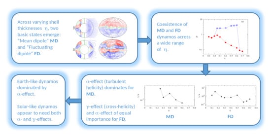
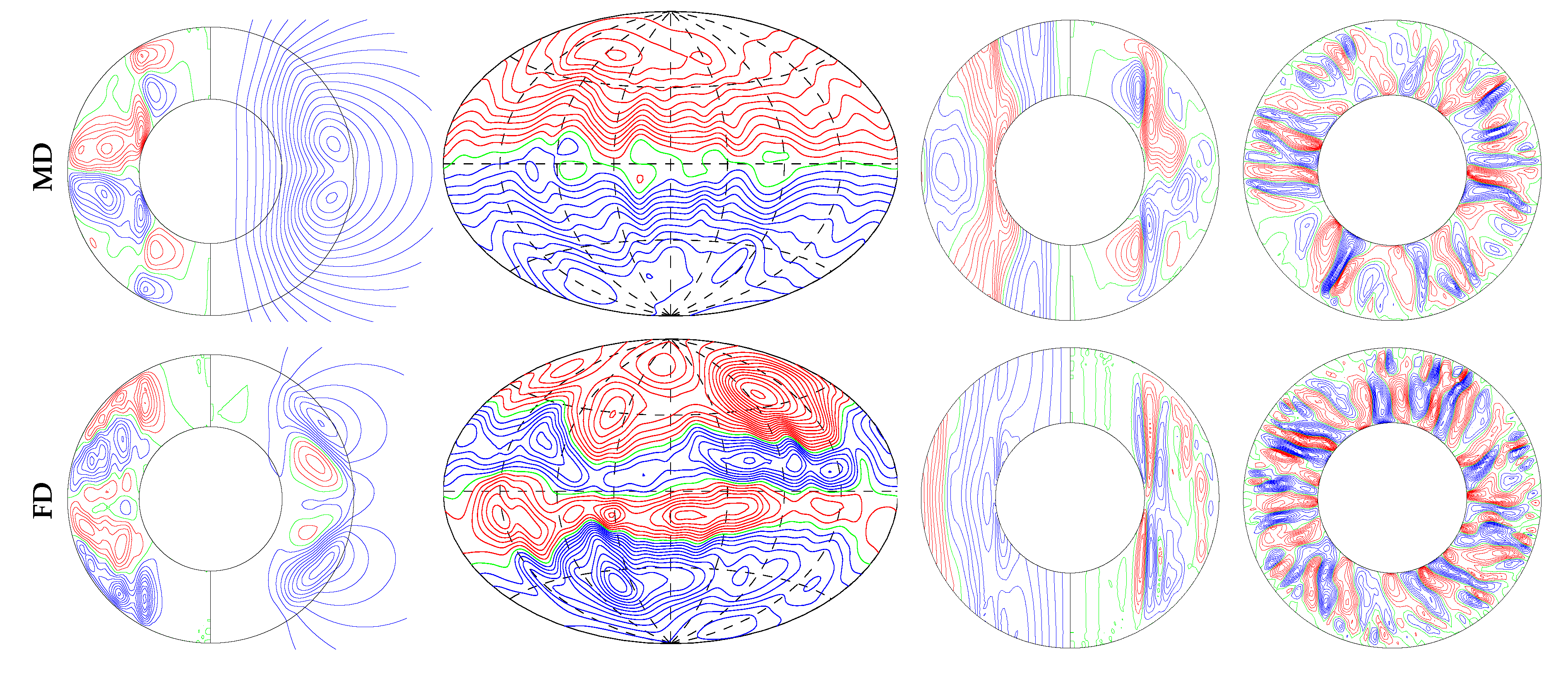
3. Results
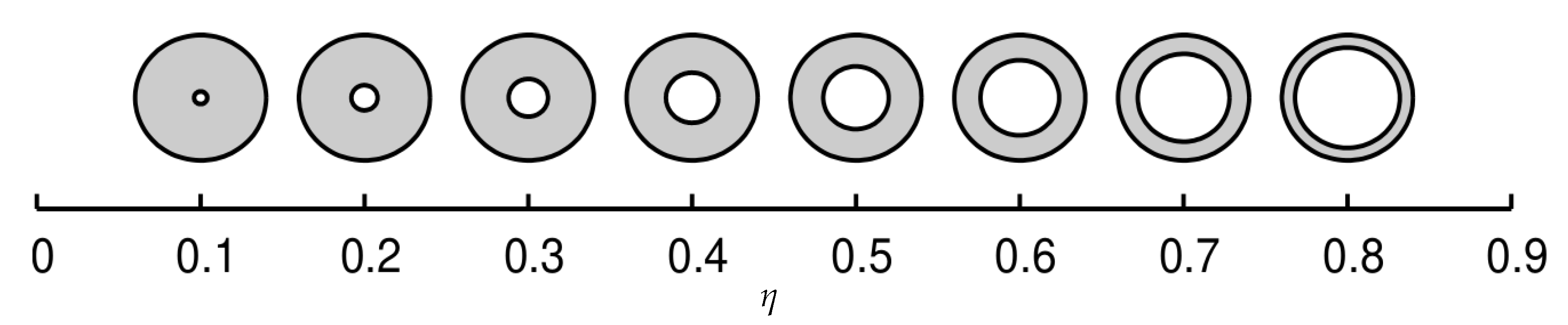
3.1. Parameter Values Used
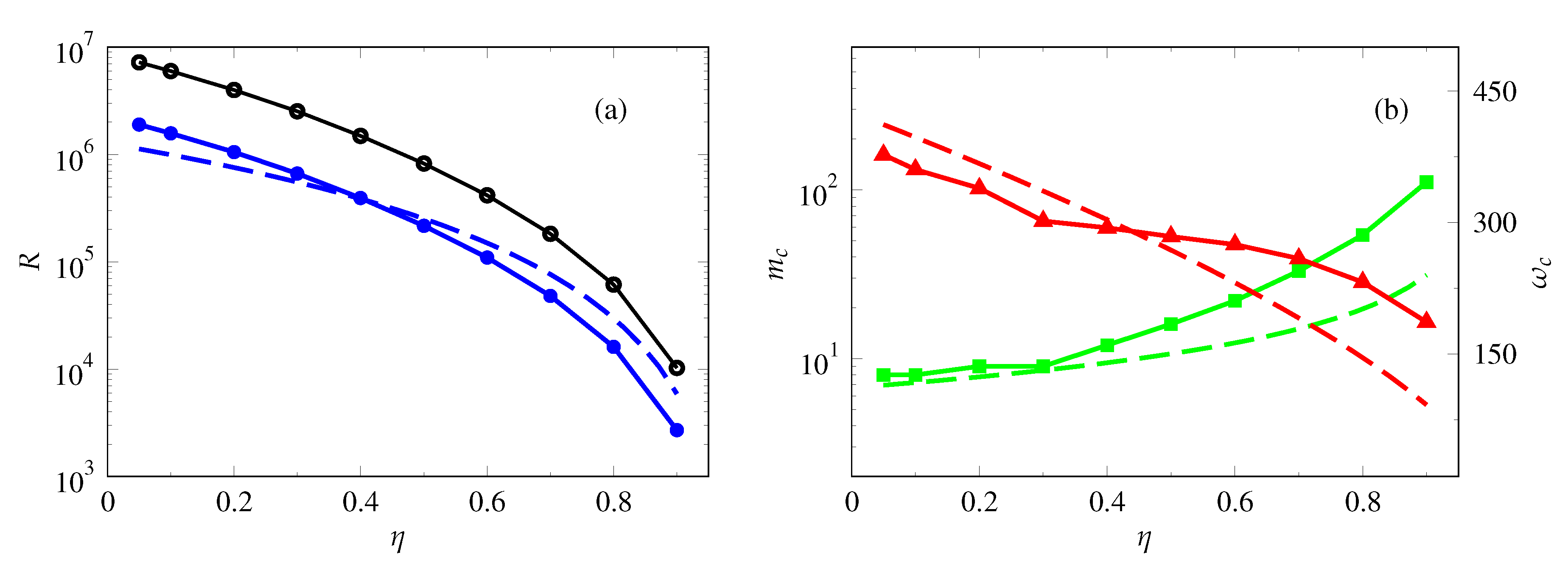
3.2. Linear Onset of Thermal Convection
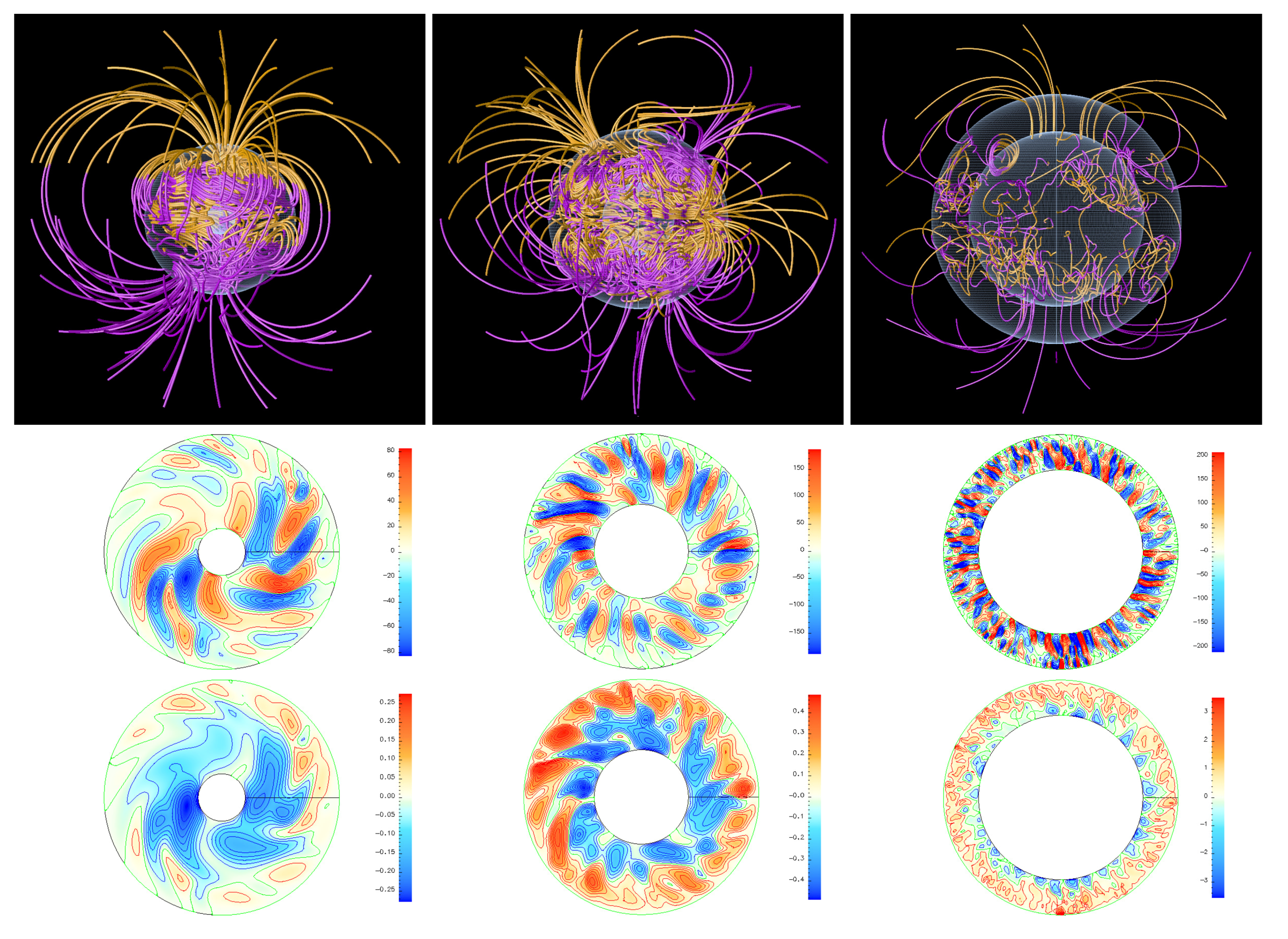
3.3. Finite-Amplitude Convection and Dynamo Features
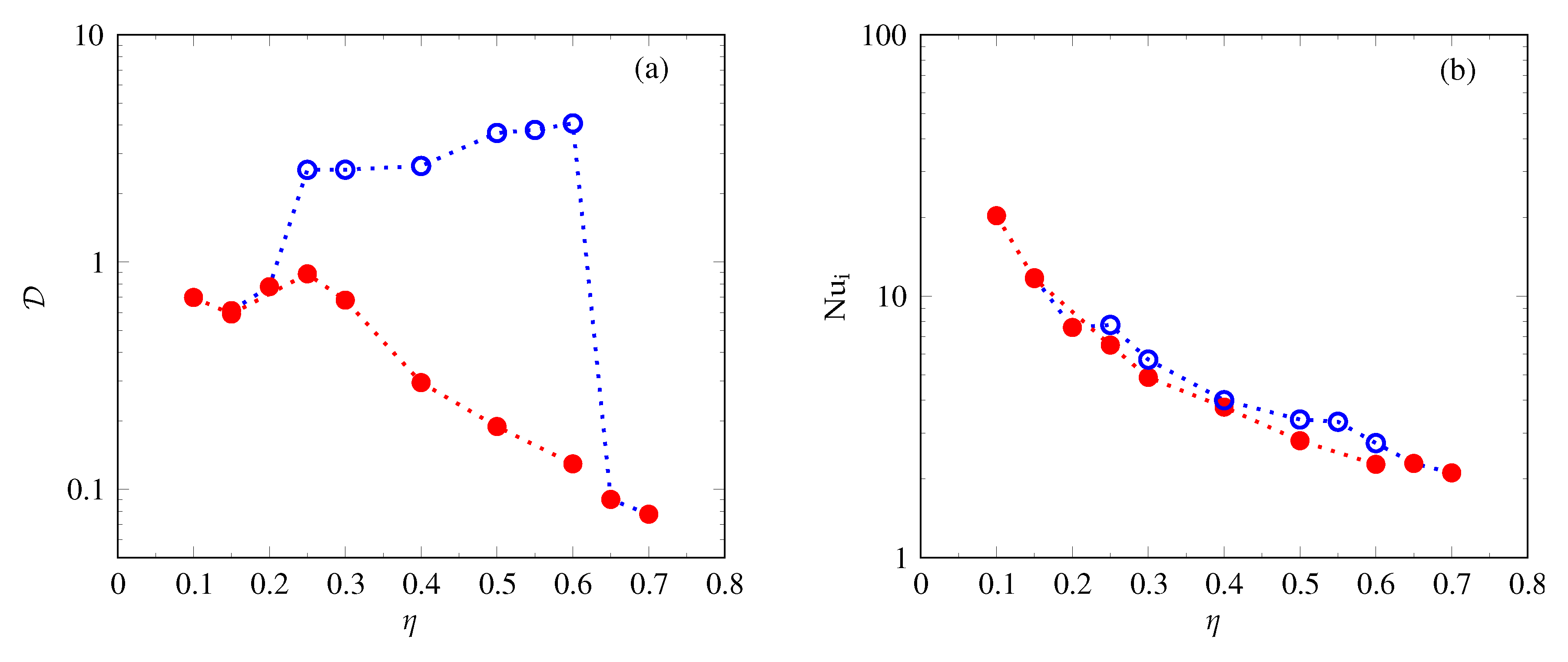
3.4. Bistability and General Effects of Shell Thickness Variation
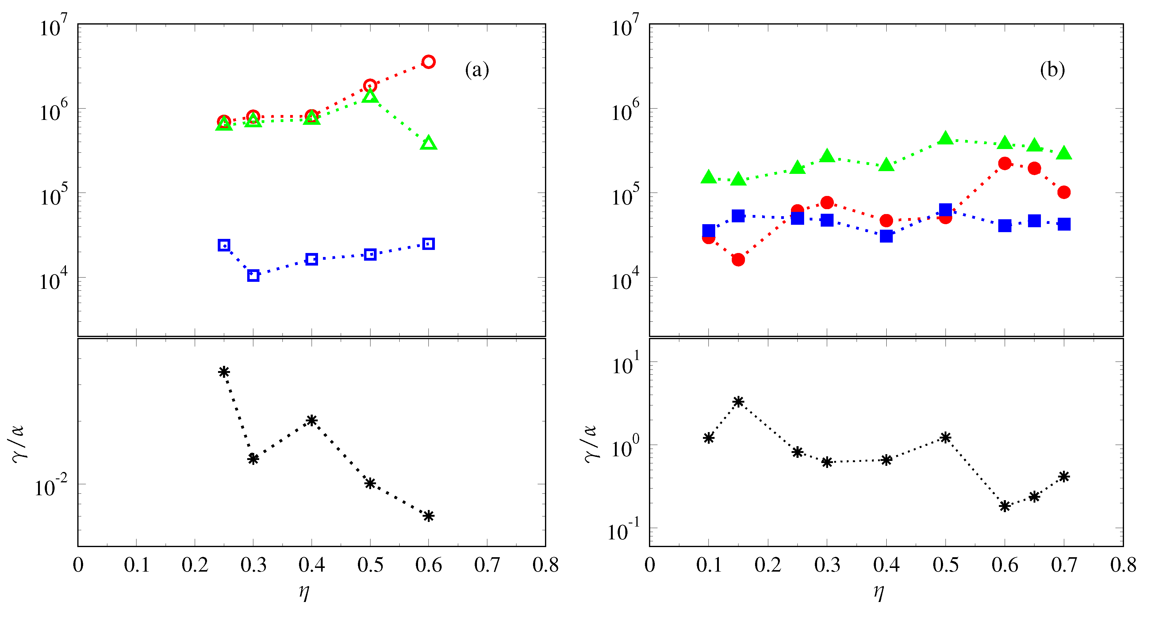
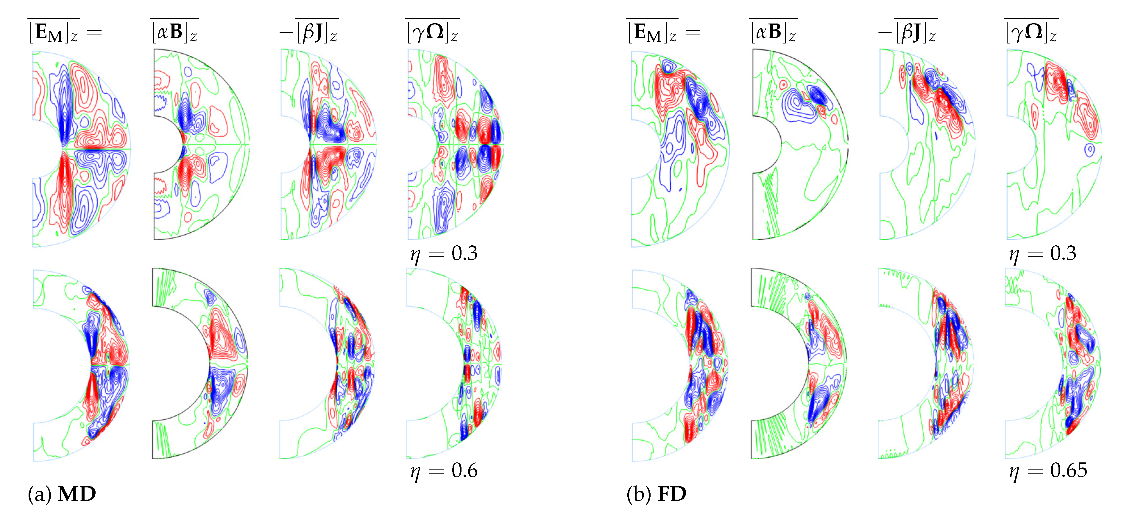
3.5. The Cross-Helicity Effect
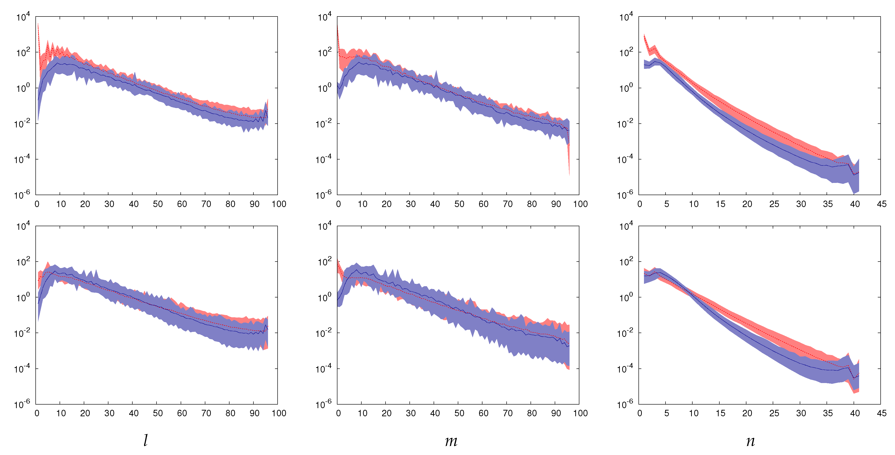
3.6. Properties and Relative Importance of Cross-Helicity
4. Summary and Discussion
- (a)
- Critical parameter values for onset of convection determined numerically as functions of the shell radius ratio, .
- (b)
- Bistability and coexistence of two distinct dynamo attractors found as a function of the shell radius ratio, .
- (c)
- Spatial distributions and time-averaged values of turbulent helicity and cross-helicity EMF effects obtained (1) for both types of dynamo attractors, as well as (2) as functions of the shell radius ratio, .
Author Contributions
Funding
Acknowledgments
Conflicts of Interest
Abbreviations
| MD | Mean Dipolar Dynamo |
| FD | Fluctuating Dipolar Dynamo |
References
- Parker, E.N. Cosmical Magnetic Fields. Their Origin and Their Activity; OUP: London, UK, 1979. [Google Scholar]
- Brun, A.S.; Browning, M.K. Magnetism, dynamo action and the solar-stellar connection. Living Rev. Sol. Phys. 2017, 14. [Google Scholar] [CrossRef]
- Zwaan, C. Elements and Patterns in the Solar Magnetic Field. Annu. Rev. Astron. Astrophys. 1987, 25, 83–111. [Google Scholar] [CrossRef]
- Busse, F.; Simitev, R. Planetary Dynamos. In Treatise on Geophysics; Elsevier: Amsterdam, The Netherlands, 2015; pp. 239–254. [Google Scholar]
- Usoskin, I.G. A history of solar activity over millennia. Living Rev. Sol. Phys. 2017, 14. [Google Scholar] [CrossRef]
- Owens, M.J.; Forsyth, R.J. The Heliospheric Magnetic Field. Living Rev. Sol. Phys. 2013, 10. [Google Scholar] [CrossRef]
- Russell, C.T. The Magnetosphere. Annu. Rev. Earth Planet. Sci. 1991, 19, 169–182. [Google Scholar] [CrossRef]
- Busse, F.H.; Simitev, R. Dynamos of Giant Planets; Cambridge University Press: Cambridge, UK, 2006; pp. 467–474. [Google Scholar]
- Larmor, J. How could a rotating body such as the Sun become a magnet? Rep. Br. Assoc. 1919, 87, 159–160. [Google Scholar]
- Moffatt, H.K. Magnetic Field Generation in Electrically Conducting Fluids; Cambridge University Press: Cambridge, UK, 1978. [Google Scholar]
- Charbonneau, P. Solar Dynamo Theory. Annu. Rev. Astron. Astrophys. 2014, 52, 251–290. [Google Scholar] [CrossRef]
- Busse, F.H.; Simitev, R. Dynamos driven by convection in rotating spherical shells. Astr. Nachr. 2005, 326, 231. [Google Scholar] [CrossRef]
- Jones, C.A. 8.05-Thermal and Compositional Convection in the Outer Core. In Treatise on Geophysics, 2nd ed.; Schubert, G., Ed.; Elsevier: Amsterdam, The Netherlands, 2015; pp. 115–159. [Google Scholar]
- Wicht, J.; Sanchez, S. Advances in geodynamo modelling. Geophys. Astrophys. Fluid Dyn. 2019, 113, 2–50. [Google Scholar] [CrossRef]
- Krause, F.; Raedler, K.H. Mean-Field Magnetohydrodynamics and Dynamo Theory; Pergamon: Oxford, UK, 1980. [Google Scholar]
- Brandenburg, A. Advances in mean-field dynamo theory and applications to astrophysical turbulence. J. Plasma Phys. 2018, 84. [Google Scholar] [CrossRef]
- Moffatt, K.; Dormy, E. Self-Exciting Fluid Dynamos; Cambridge University Press: Cambridge, UK, 2019. [Google Scholar]
- Brandenburg, A.; Subramanian, K. Astrophysical magnetic fields and nonlinear dynamo theory. Phys. Rep. 2005, 417, 1–209. [Google Scholar] [CrossRef]
- Yoshizawa, A.; Yokoi, N. Turbulent Magnetohydrodynamic Dynamo for Accretion Disks Using the Cross-Helicity Effect. Astrophys. J. 1993, 407, 540. [Google Scholar] [CrossRef]
- Yokoi, N. Cross helicity and related dynamo. Geophys. Astrophys. Fluid Dyn. 2013, 107, 114–184. [Google Scholar] [CrossRef]
- Pipin, V.V.; Yokoi, N. Generation of a Large-scale Magnetic Field in a Convective Full-sphere Cross-helicity Dynamo. Astrophys. J. 2018, 859, 18. [Google Scholar] [CrossRef]
- Thompson, M.J.; Toomre, J.; Anderson, E.R.; Antia, H.M.; Berthomieu, G.; Burtonclay, D.; Chitre, S.M.; Christensen-Dalsgaard, J.; Corbard, T.; DeRosa, M.; et al. Differential Rotation and Dynamics of the Solar Interior. Science 1996, 272, 1300–1305. [Google Scholar] [CrossRef]
- Schou, J.; Antia, H.M.; Basu, S.; Bogart, R.S.; Bush, R.I.; Chitre, S.M.; Christensen-Dalsgaard, J.; Mauro, M.P.D.; Dziembowski, W.A.; Eff-Darwich, A.; et al. Helioseismic Studies of Differential Rotation in the Solar Envelope by the Solar Oscillations Investigation Using the Michelson Doppler Imager. Astrophys. J. 1998, 505, 390–417. [Google Scholar] [CrossRef]
- Busse, F.H.; Simitev, R. Parameter dependences of convection-driven dynamos in rotating spherical fluid shells. Geophys. Astrophys. Fluid Dyn. 2006, 100, 341. [Google Scholar] [CrossRef][Green Version]
- Simitev, R.D.; Busse, F.H. How far can minimal models explain the solar cycle? Astrophys. J. 2012, 749, 9. [Google Scholar] [CrossRef]
- Hamba, F. Turbulent dynamo effect and cross helicity in magnetohydrodynamic flows. Phys. Fluids Fluid Dyn. 1992, 4, 441–450. [Google Scholar] [CrossRef]
- Yokoi, N.; Balarac, G. Cross-helicity effects and turbulent transport in magnetohydrodynamic flow. J. Phys. Conf. Ser. 2011, 318, 072039. [Google Scholar] [CrossRef]
- Rüdiger, G.; Küker, M.; Schnerr, R.S. Cross helicity at the solar surface by simulations and observations. Astron. Astrophys. 2012, 546, A23. [Google Scholar] [CrossRef][Green Version]
- Simitev, R.D.; Busse, F.H. Bistability and hysteresis of dipolar dynamos generated by turbulent convection in rotating spherical shells. EPL (Europhys. Lett.) 2009, 85, 19001. [Google Scholar] [CrossRef]
- Busse, F.H.; Simitev, R. Remarks on some typical assumptions in dynamo theory. Geophys. Astrophys. Fluid Dyn. 2011, 105, 234. [Google Scholar] [CrossRef]
- Simitev, R.D.; Busse, F.H. Bistable attractors in a model of convection-driven spherical dynamos. Phys. Scr. 2012, 86, 018409. [Google Scholar] [CrossRef][Green Version]
- Busse, F.H.; Simitev, R. Toroidal flux oscillations as possible causes of geomagnetic excursions and reversals. Phys. Earth Planet. Inter. 2008, 168, 237. [Google Scholar] [CrossRef][Green Version]
- Matilsky, L.I.; Toomre, J. Exploring Bistability in the Cycles of the Solar Dynamo through Global Simulations. Astrophys. J. 2020, 892, 106. [Google Scholar] [CrossRef]
- Simitev, R.; Busse, F.H. Prandtl-number dependence of convection-driven dynamos in rotating spherical fluid shells. J. Fluid Mech. 2005, 532, 365. [Google Scholar] [CrossRef]
- Mather, J.F.; Simitev, R.D. Regimes of thermo-compositional convection and related dynamos in rotating spherical shells. Geophys. Astrophys. Fluid Dyn. 2020, 1–24. [Google Scholar] [CrossRef]
- Busse, F.H. Homogeneous Dynamos in Planetary Cores and in the Laboratory. Annu. Rev. Fluid Mech. 2000, 32, 383–408. [Google Scholar] [CrossRef]
- Dormy, E.; Simitev, R.; Busse, F.; Soward, A. Dynamics of Rotating Fluids. In Mathematical Aspects of Natural Dynamos; Chapman and Hall/CRC: Boca Raton, FL, USA, 2007; pp. 120–198. [Google Scholar]
- Roberts, P.H.; King, E.M. On the genesis of the Earth’s magnetism. Rep. Prog. Phys. 2013, 76, 096801. [Google Scholar] [CrossRef]
- Grote, E.; Busse, F.; Tilgner, A. Regular and chaotic spherical dynamos. Phys. Earth Planet. Inter. 2000, 117, 259–272. [Google Scholar] [CrossRef]
- Simitev, R.; Busse, F.H. Patterns of convection in rotating spherical shells. New J. Phys. 2003, 5, 97. [Google Scholar] [CrossRef]
- Simitev, R.; Busse, F.; Grote, E. Convection in rotating spherical shells and its dynamo action. In Earth’s Core and Lower Mantle; CRC Press: Boca Raton, FL, USA, 2003; pp. 130–152. [Google Scholar]
- Simitev, R.; Busse, F.H. Solar cycle properties described by simple convection-driven dynamos. Phys. Scr. 2012, 86, 018407. [Google Scholar] [CrossRef]
- Tilgner, A. Spectral methods for the simulation of incompressible flows in spherical shells. Int. J. Numer. Meth. Fluids 1999, 30, 713–724. [Google Scholar] [CrossRef]
- Marti, P.; Schaeffer, N.; Hollerbach, R.; Cébron, D.; Nore, C.; Luddens, F.; Guermond, J.L.; Aubert, J.; Takehiro, S.; Sasaki, Y.; et al. Full sphere hydrodynamic and dynamo benchmarks. Geophys. J. Int. 2014, 197, 119–134. [Google Scholar] [CrossRef]
- Matsui, H.; Heien, E.; Aubert, J.; Aurnou, J.M.; Avery, M.; Brown, B.; Buffett, B.A.; Busse, F.; Christensen, U.R.; Davies, C.J.; et al. Performance benchmarks for a next generation numerical dynamo model. Geochem. Geophys. Geosyst. 2016, 17, 1586–1607. [Google Scholar] [CrossRef]
- Silva, L.A.C.; Simitev, R.D. Pseudo-Spectral Code For Numerical Simulation Of Nonlinear Thermo-Compositional Convection and Dynamos in Rotating Spherical Shells; University of Glasgow: Glasgow, UK, 2018. [Google Scholar] [CrossRef]
- Christensen, U.; Olson, P.; Glatzmaier, G.A. Numerical modelling of the geodynamo: A systematic parameter study. Geophys. J. Int. 1999, 138, 393–409. [Google Scholar] [CrossRef]
- Silva, L.; Mather, J.F.; Simitev, R.D. The onset of thermo-compositional convection in rotating spherical shells. Geophys. Astrophys. Fluid Dyn. 2019, 113, 377–404. [Google Scholar] [CrossRef]
- Busse, F.H.; Simitev, R. Inertial convection in rotating fluid spheres. J. Fluid Mech. 2004, 498, 23–30. [Google Scholar] [CrossRef]
- Silva, L.A.C.; Simitev, R.D. Spectral Code for Linear Analysis of The Onset of Thermo-Compositional Convection in Rotating Spherical Fluid Shells; University of Glasgow: Glasgow, UK, 2018. [Google Scholar] [CrossRef]
- Zhang, K.K.; Busse, F.H. On the onset of convection in rotating spherical shells. Geophys. Astrophys. Fluid Dyn. 1987, 39, 119–147. [Google Scholar] [CrossRef]
- Roberts, P.H. On the Thermal Instability of a Rotating-Fluid Sphere Containing Heat Sources. Philos. Trans. R. Soc. Math. Phys. Eng. Sci. 1968, 263, 93–117. [Google Scholar] [CrossRef]
- Busse, F.H. Thermal instabilities in rapidly rotating systems. J. Fluid Mech. 1970, 44, 441. [Google Scholar] [CrossRef]
- Soward, A.M. On the Finite amplitude thermal instability of a rapidly rotating fluid sphere. Geophys. Astrophys. Fluid Dyn. 1977, 9, 19–74. [Google Scholar] [CrossRef]
- Jones, C.A.; Soward, A.M.; Mussa, A.I. The onset of thermal convection in a rapidly rotating sphere. J. Fluid Mech. 2000, 405, 157–179. [Google Scholar] [CrossRef]
- Dormy, E.; Soward, A.M.; Jones, C.A.; Jault, D.; Cardin, P. The onset of thermal convection in rotating spherical shells. J. Fluid Mech. 2004, 501, 43–70. [Google Scholar] [CrossRef]
- Yano, J.I. Asymptotic theory of thermal convection in rapidly rotating systems. J. Fluid Mech. 1992, 243, 103. [Google Scholar] [CrossRef]
- Christensen, U.R.; Aubert, J. Scaling properties of convection-driven dynamos in rotating spherical shells and application to planetary magnetic fields. Geophys. J. Int. 2006, 166, 97–114. [Google Scholar] [CrossRef]
- Olson, P.L.; Glatzmaier, G.A.; Coe, R.S. Complex polarity reversals in a geodynamo model. Earth Planet. Sci. Lett. 2011, 304, 168–179. [Google Scholar] [CrossRef]
- Yokoi, N. Turbulence, Transport and Reconnection. In Topics in Magnetohydrodynamic Topology, Reconnection and Stability Theory; MacTaggart, D., Hillier, A., Eds.; Springer: Cham, Switzerland, 2020; pp. 177–265. [Google Scholar]
- Yoshizawa, A. Self-consistent turbulent dynamo modeling of reversed field pinches and planetary magnetic fields. Phys. Fluids Plasma Phys. 1990, 2, 1589–1600. [Google Scholar] [CrossRef]
- Christensen-Dalsgaard, J.; Dappen, W.; Ajukov, S.V.; Anderson, E.R.; Antia, H.M.; Basu, S.; Baturin, V.A.; Berthomieu, G.; Chaboyer, B.; Chitre, S.M.; et al. The Current State of Solar Modeling. Science 1996, 272, 1286–1292. [Google Scholar] [CrossRef]
- Simitev, R.D.; Kosovichev, A.G.; Busse, F.H. Dynamo effects near the transition from solar to anti-solar differential rotation. Astrophys. J. 2015, 810, 80. [Google Scholar] [CrossRef]
- MacTaggart, D.; Gregory, S.G.; Neukirch, T.; Donati, J.F. Magnetohydrostatic modelling of stellar coronae. Mon. Not. RAS 2015, 456, 767–774. [Google Scholar] [CrossRef]
- Driscoll, P.E. Simulating 2 Ga of geodynamo history. Geophys. Res. Lett. 2016, 43, 5680–5687. [Google Scholar] [CrossRef]
- Landeau, M.; Aubert, J.; Olson, P. The signature of inner-core nucleation on the geodynamo. Earth Planet. Sci. Lett. 2017, 465, 193–204. [Google Scholar] [CrossRef]


| Notation | Quantity | Notation | Quantity |
|---|---|---|---|
| Spherical polar coordinates | Background temperature distribution | ||
| t | Time | Temperature inner, outer boundary | |
| Position vector wrt centre of sphere | q | Density of uniformly distributed heat sources | |
| d | Thickness of the spherical shell | Thermal diffusivity | |
| , | Inner and outer radii of the shell | Kinematic viscosity | |
| Velocity field perturbation | Magnetic permeability | ||
| Magnetic flux density perturbation | Specific heat at constant pressure | ||
| Temperature perturbation from the background state | Gravitational acceleration magnitude | ||
| Effective pressure | ∂ | Partial derivative notation |
| Quantity | Unit |
|---|---|
| Length | d |
| Time | |
| Temperature | |
| Magnetic flux density |
Publisher’s Note: MDPI stays neutral with regard to jurisdictional claims in published maps and institutional affiliations. |
© 2020 by the authors. Licensee MDPI, Basel, Switzerland. This article is an open access article distributed under the terms and conditions of the Creative Commons Attribution (CC BY) license (http://creativecommons.org/licenses/by/4.0/).
Share and Cite
Silva, L.; Gupta, P.; MacTaggart, D.; Simitev, R.D. Effects of Shell Thickness on Cross-Helicity Generation in Convection-Driven Spherical Dynamos. Fluids 2020, 5, 245. https://doi.org/10.3390/fluids5040245
Silva L, Gupta P, MacTaggart D, Simitev RD. Effects of Shell Thickness on Cross-Helicity Generation in Convection-Driven Spherical Dynamos. Fluids. 2020; 5(4):245. https://doi.org/10.3390/fluids5040245
Chicago/Turabian StyleSilva, Luis, Parag Gupta, David MacTaggart, and Radostin D. Simitev. 2020. "Effects of Shell Thickness on Cross-Helicity Generation in Convection-Driven Spherical Dynamos" Fluids 5, no. 4: 245. https://doi.org/10.3390/fluids5040245
APA StyleSilva, L., Gupta, P., MacTaggart, D., & Simitev, R. D. (2020). Effects of Shell Thickness on Cross-Helicity Generation in Convection-Driven Spherical Dynamos. Fluids, 5(4), 245. https://doi.org/10.3390/fluids5040245