Modelling a Moving Propeller System in a Stratified Fluid Using OpenFOAM  ^†

Abstract

Moving propeller systems can introduce significant disturbances in stratified environments by mixing the surrounding fluid. Restorative buoyancy forces subsequently act on this region/patch of mixed fluid, causing it to eventually collapse vertically and spread laterally in order to recover the original stratification. This work describes the use of an OpenFOAM solver, modified using existing functionality, to simulate a moving propeller system in a stratified environment. Its application considers a rotating KCD-32 propeller in a laboratory-scale wave tank which mimics published experiments on mixed patch collapse. The numerically-predicted collapse behaviour is compared with empirical data and scaling laws. The results agree closely, both qualitatively and quantitatively, thereby representing a successful step towards the validation of the numerical model.

1. Introduction

Stratified environments are created when a fluid’s temperature and/or salinity, and therefore density, changes with respect to depth [1]. A propeller system moving through such an environment is capable of rapidly mixing the surrounding fluid across isopycnals, yielding a so-called ‘mixed patch’ of near-uniform density in its wake. The mixed patch is subjected to buoyancy forces which attempt to restore the stratification to its initial (unperturbed) state. This results in the patch collapsing vertically and spreading out laterally, radiating internal waves in the process [2,3].

Several important stages in the collapse process have been identified through experiments and numerical models [4,5,6,7]. At early times, the turbulent kinetic energy introduced by the sudden mixing causes the patch to grow in size. This process increases the potential energy stored in the mixed patch. After the passage of the mixing source, buoyancy forces eventually overcome inertia and the patch begins to collapse vertically in an effort to restore the stratification to its equilibrium state. At later times the flow comprises ‘pancake’-like eddies characterised by vertical vorticity [8]. However, many studies have not focussed on the effects of swirl from propeller systems, which may have a significant effect on the collapse and post-collapse behaviour.

Numerical approaches to modelling the action of propeller motion on fluids include actuator line and actuator disk models [9,10,11,12]; blade element momentum theory [13,14,15,16]; and models in which the propeller blades are fully resolved by the computational mesh and dynamically rotated [17,18,19]. The latter approach was considered by Colley [17], for example, who modelled a 5-blade KCD-32 series propeller using OpenFOAM; an open-source fluid dynamics modelling framework [20,21,22]. However, the environment was not stratified. The behaviour of mixed patch collapse under buoyancy could therefore not be considered.

The work presented herein concerns the application of buoyantPimpleFoam, an existing transient flow solver in the OpenFOAM modelling framework which takes buoyancy effects into account. Modifications were made to the buoyantPimpleFoam solver in order to use the dynamic mesh (DyM) and arbitrary mesh interface (AMI) functionality readily available in OpenFOAM [23,24,25,26]. The use of DyM and AMI enabled support for rotating computational meshes (and therefore a rotating propeller) and the representation of a propeller’s hydrodynamic wake in a stratified environment. A step towards validating the numerical model is achieved by simulating the collapse of a mixed patch generated by a propeller, equipped with five KCD-32 blades, in a laboratory-scale stratified wave tank. The qualitative behaviour of the mixed patch throughout time is compared with similar experimental studies by Merritt [4] and Lin & Pao [5]. In particular, the numerical predictions are validated against empirical data and scaling laws describing the height and width of the mixed patch throughout its evolution. However, one difference between the model and the experiments is the use of a rotating KCD-32 propeller rather than an oscillating grid to generate the mixed patch. Furthermore, this numerical study only considers a single value of the Brunt–Väisälä frequency and Froude number, rather than a range of values. The model, once sufficiently validated, could potentially be applied at a larger scale to understand the collapse of mixed patches generated by underwater bluff bodies [7] or marine power turbines [27], for example.

The remainder of this paper is organised as follows. Section 2 briefly describes the numerical model, including the governing equations. Details on the computer-aided design (CAD) and meshing process are provided along with a description of how the simulations were set up. The numerical results are presented in Section 3. The various stages of the mixed patch collapse process are successfully observed in the model. The numerically-predicted height and width of the mixed patch agree well with the scaling laws of Merritt [4] and Lin & Pao [5]. The paper closes with some concluding remarks in Section 4.

2. Method

2.1. Model

The OpenFOAM modelling framework [20,21,22] was used to conduct the numerical study. In particular, a transient flow solver capable of simulating buoyant flow, buoyantPimpleFoam, was modified for the purpose of modelling a moving propeller in a stratified environment. The development version of OpenFOAM, available from https://github.com/OpenFOAM/OpenFOAM-dev, was forked (copied to a local repository) from Git commit 409548cbccac and the source code was subsequently modified to make use of the existing DyM and AMI functionality [23,24,25,26]. Similar use cases of this functionality can be found in the rhoPimpleFoam and interFoam solvers, for example. Note that, since this work was conducted, a more recent development version now includes support for moving meshes in the buoyantPimpleFoam solver; this support was added independently of this work (see Git commit 38fff77d3537 by Henry Weller).

The numerical model considers the Navier–Stokes equations, governing the conservation laws of mass and momentum, with the Boussinesq approximation applied [28]. The fluid under consideration is inhomogeneous with small vertical density variations arising from its stratification. However, the Boussinesq approximation assumes that such density variations are small enough to be neglected except within the buoyancy term [29]. Therefore, the governing equations reduce to their incompressible form given by

$$\frac{\partial u_i}{\partial x_i}=0,$$

(1)

$$\frac{\partial u_i}{\partial t}+\frac{\partial \left(u_i{u}_j\right)}{\partial x_j}=-\frac{1}{{\rho }_0}\frac{\partial p}{\partial x_i}+\frac{\rho }{{\rho }_0}{g}_i+\frac{\partial {\tau }_{ij}}{\partial x_j},$$

(2)

where $\rho$ is the density of the fluid, ${\rho }_0$ = 1000 kgm${}^{-3}$ is the reference density, $u=[u_1,u_2,u_3]$ is the flow velocity, p is pressure, g = [0, 0, −9.81] ms${}^{-2}$ is the acceleration due to gravity, $x=[x_1,x_2,x_3]$ is the spatial coordinate, and t denotes time [30]. The stress tensor $\tau$ is based on the fluid’s kinematic viscosity $\nu$ = 10${}^{-6}$ m${}^2$s${}^{-1}$. Summation is implied over repeated indices. Note also that $x_1$, $x_2$ and $x_3$ are respectively referred to as x, y and z throughout the remainder of this paper. Similarly, $u_x$, $u_y$ and $u_z$ are used to respectively refer to $u_1$, $u_2$ and $u_3$.

2.2. Equation of State

A linear equation of state was used to compute the density field $\rho$, based on the temperature T, as follows

$$\rho \left(T\right)={\rho }_0\left(1-\alpha (T-T_0)\right),$$

(3)

where $\alpha$ = 10${}^{-4}$ K${}^{-1}$ is the thermal expansion coefficient [31] and $T_0$ = 293.15 K is the reference temperature.

2.3. Domain

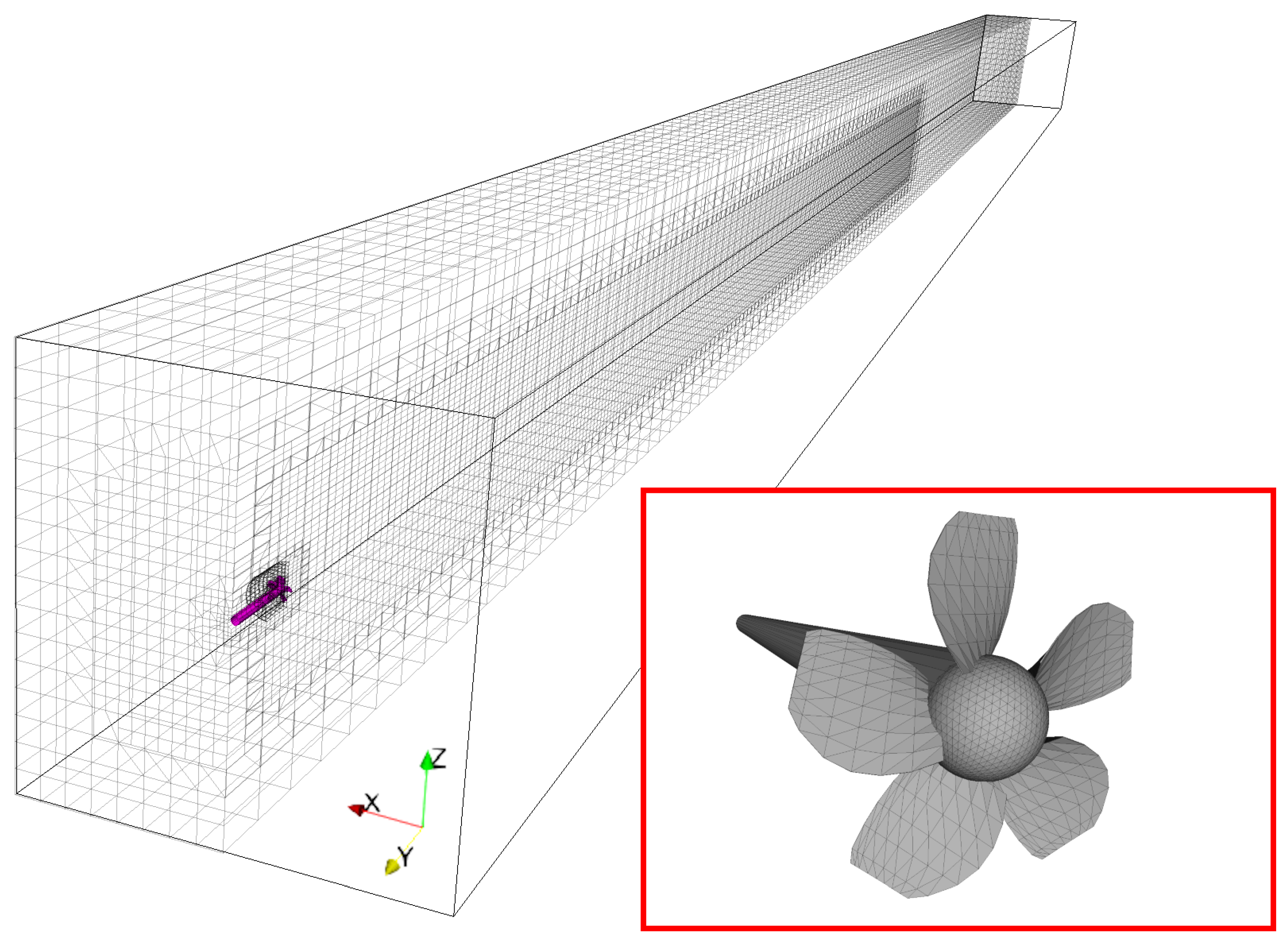
A three-dimensional cuboid domain representing the laboratory-scale wave tank of Merritt [4] was considered, with dimensions $-0.05\le x\le 0.05$ m, $-2.0\le y\le 0.02$ m, and $-0.1\le z\le 0$ m. The propeller’s hub was centred at (0, 0, −0.05) as shown in Figure 1. The model was implemented in a reference frame where the fluid flows through a fixed rotating propeller system (rather than a propeller travelling through quiescent fluid). Inlet and outlet boundary planes were therefore defined at y = 0.02 m and y = −2 m, respectively.

The computational grid included a series of mesh refinements performed using the OpenFOAM meshing algorithms. A coarse discretisation was first performed by introducing a uniform structured grid of 16 × 128 × 16 (∼32,000) solution points throughout the entire domain. A cylindrical region of enhanced resolution which encapsulated the propeller was then introduced. A cuboidal region of high resolution was also placed downstream to resolve the mixing action of the propeller. Cells were then removed using OpenFOAM’s snappyHexMesh utility to create a propeller-shaped void in the mesh. The cells in the vicinity of the propeller were further refined, with the first layer of cells typically having a non-dimensional thickness ($y^{+}$ value) of ∼0.8 (approximately 10${}^{-3}$ m). The resulting mesh comprised a total of approximately 346,000 solution points.

2.4. Propeller

The propeller featured five KCD-32 blades, appropriately scaled-down to fit the laboratory-scale domain. These blades, defined by [32], were meshed and written to a file in stereolithography (STL) format. Each blade had an approximate length of 0.0022 m. A shaft and hub (0.02 m in length, 0.002 m in diameter, inset in Figure 1) were designed using FreeCAD (https://www.freecadweb.org/) [33]. These were used to mount each of the blades to form the complete propeller system. The total diameter D of the propeller was therefore approximately 0.0064 m, similar to that of the oscillating grid (D = 0.00635 m) used in the experiments of Merritt [4].

The propeller was rotated at a rate of 120 revolutions per minute (rpm). The motion of the propeller was accomplished using the DyM and AMI functionality within OpenFOAM; this functionality rotated the vertices of the cylindrical region (encapsulating the propeller) embedded in the computational mesh, and also enabled the finite volume fluxes to be interpolated from the former mesh topography onto the modified (rotated) topography [23,24,25,26].

2.5. Initial Conditions

The initial velocity field assumed a uniform downstream flow throughout the entire domain such that $u(x,t=0)=[0,-0.01,0]$ ms${}^{-1}$. The pressure field p was initially set to zero, but throughout the simulation the solver computed this field based on the hydrostatic pressure and any pressure fluctuations encountered (such as those at the propeller blades).

The temperature of the fluid at the bottom of the wave tank $T_b$ was set to 293.15 K. The temperature increased linearly towards the surface of the wave tank, with the surface temperature $T_s$ = 294.45 K. This yielded a stable stratification. Internal waves oscillate in a stratified environment with a maximum frequency known as the Brunt–Väisälä frequency [1], defined as

$$N=\frac{1}{2\pi }\sqrt{-\frac{|g_z|}{{\rho }_0}\frac{\partial \rho }{\partial z}}.$$

(4)

The Brunt–Väisälä frequency of the stratification considered here was N = 0.018 s${}^{-1}$ (i.e., a buoyancy period of ∼55 s, as per one of the experiments by Merritt [4]).

The Froude number expresses the ratio between inertia and buoyancy forces. When based on the Brunt–Väisälä frequency N and the diameter of the propeller D, it is defined as

$$\mathrm{Fr}=\frac{U}{ND},$$

(5)

where U is the free-stream flow speed of 0.01 ms${}^{-1}$. For this particular setup, $\mathrm{Fr}$ = 87.6 which is within the range of Froude numbers considered by Merritt [4] and Lin & Pao [5].

2.6. Boundary Conditions

The inlet flow speed was set to a constant 0.01 ms${}^{-1}$, while a zero pressure boundary condition at the outlet allowed fluid to flow freely out of the domain. Free-slip conditions were assumed at the walls of the domain, representing the smooth walls of the wave tank. The temperature field at the top and bottom of the tank was set to 294.45 K and 293.15 K, respectively, while a zero-gradient condition was applied to all other walls of the domain. A zero movingWallVelocity boundary condition was enforced at the propeller. A cyclicAMI boundary condition was applied to enable the rotation of the propeller.

2.7. Discretisation

OpenFOAM uses a finite volume method to spatially discretise the domain. Upwind conditions were applied at the faces between each computational cell [34].

The forward Euler method was chosen to temporally discretise the governing equations and advance the simulation forwards in time until t = 200 s. This time-frame was sufficient to allow the mixed patch and its various stages of evolution to become established throughout the length of the domain. The timestep $\Delta t$ was automatically adapted throughout the simulation, subject to a maximum Courant number constraint of 2.0.

2.8. Solution Algorithms

The PIMPLE algorithm was used to iteratively solve the incompressible Navier–Stokes equations. Two iterations of the PIMPLE algorithm were performed per timestep. Note that PIMPLE is a combination of the PISO (Pressure Implicit with Splitting of Operator) and SIMPLE (Semi-Implicit Method for Pressure Linked Equations) algorithms [34,35].

The PIMPLE algorithm requires the solution to several systems of equations using numerical linear algebra methods. The stabilised biconjugate gradient method, preconditioned with incomplete lower–upper (LU) factorisation, was used to solve the velocity field. The pressure field was solved using the conjugate gradient method, preconditioned with incomplete Cholesky factorisation [36].

2.9. Hardware

The numerical model was executed in parallel over 18 cores, embedded in a single Intel^® Core^TM i9-9980XE processor, using the Message Passing Interface (MPI) and 64 GB of random-access memory (RAM). The model required approximately 5 days to complete a simulation.

3. Results

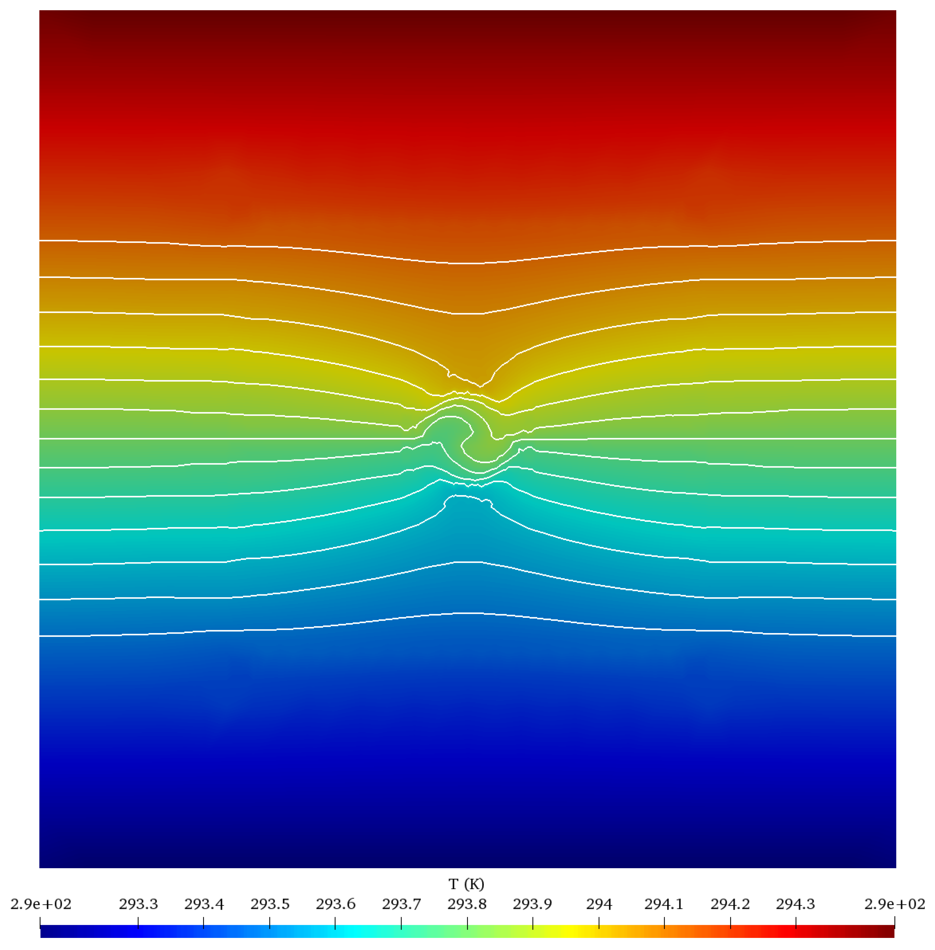
Between t = 0 and t = 200 s the motion of the propeller successfully mixed the stratified fluid to create a mixed patch. The rotating blades rapidly transported warmer fluid situated above the propeller into the lower, cooler part of the domain, and vice-versa. This is visualised by the warped contours in the centre of Figure 2. Similar temperature profiles have been observed in propeller studies involving actuator line models [11,12]. The temperature of the patch was not perfectly uniform as a result of this continuous entrainment from the undisturbed regions of the stratification.

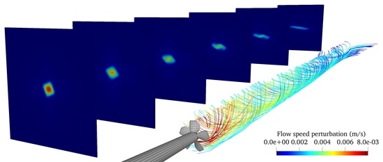
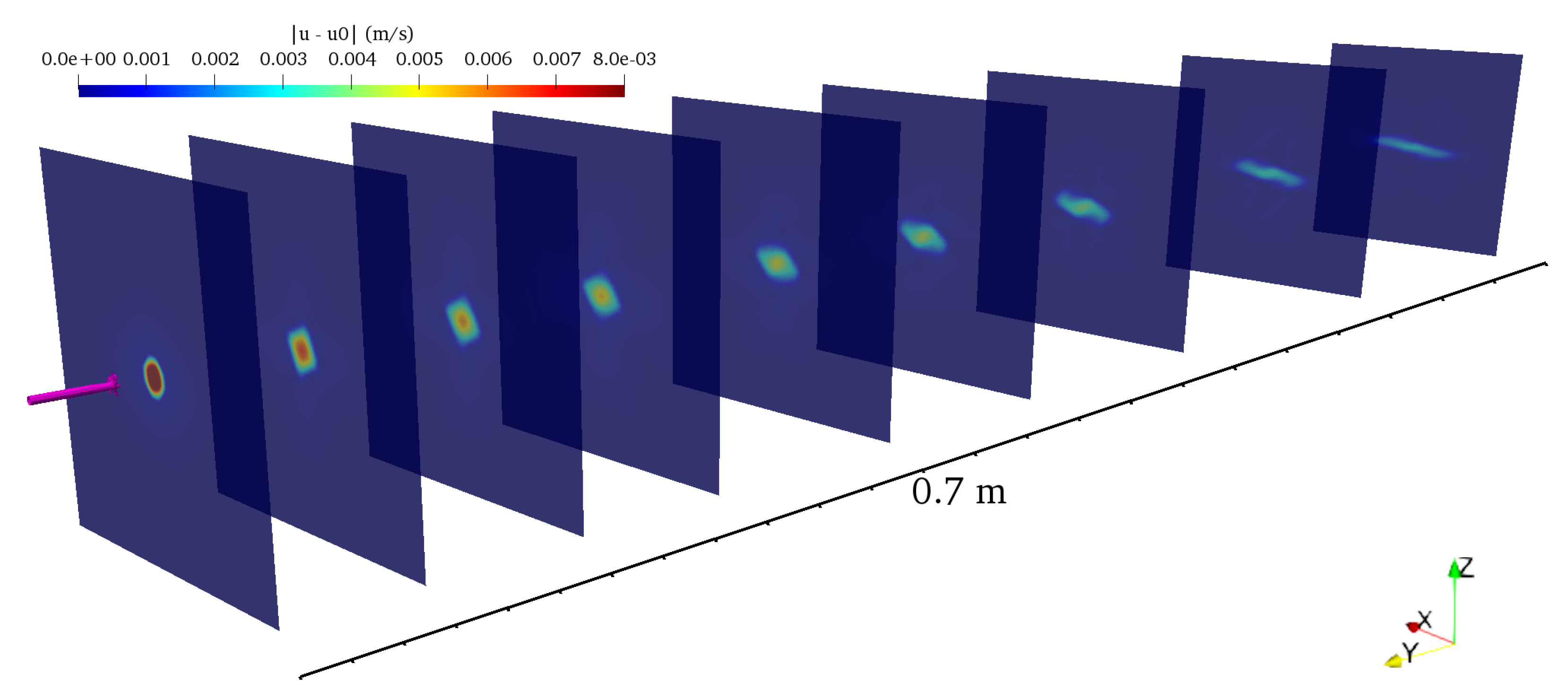
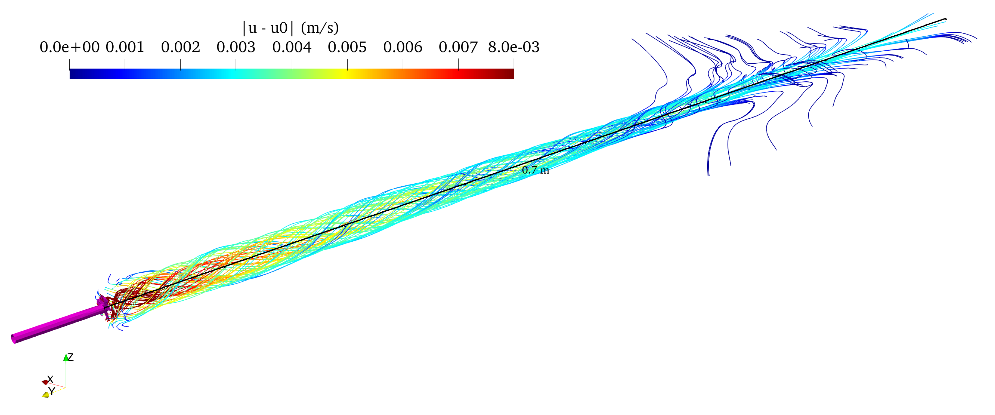
Experimental studies have shown that a mixed patch undergoes several stages of evolution [4,5]. Immediately downstream of the mixing source (i.e., the propeller), the developing mixed patch expands (both vertically and horizontally) in a similar manner to that of a mixed patch developing in a non-stratified environment. This growth is driven by the conversion of the turbulent kinetic energy provided by the propeller into potential energy. The results from the numerical simulation agree well with this observation. The flow speed perturbation field $∥u-u_0∥$ is used to illustrate this behaviour in Figure 3 and Figure 4, where $u_0\equiv u(t=0)$ and $∥·∥$ denote the Euclidean norm.

Further downstream the kinetic energy provided by the propeller is no longer sufficient to sustain the patch’s growth. Buoyancy forces begin to dominate and the patch subsequently collapses vertically in order to restore the original stratification. This in turn induces lateral motions such that the patch continues to widen at a much faster rate. Once again, the numerical results in Figure 3 and Figure 4 reinforce the experimental observations. However, unlike the experiments which considered a patch generated by a moving grid [4,5], the propeller-generated patch was characterised by a significant amount of swirl/vorticity which caused it to become slightly asymmetric in shape. Nevertheless, the stratification continued to recover as expected, with internal waves persisting within the wave tank.

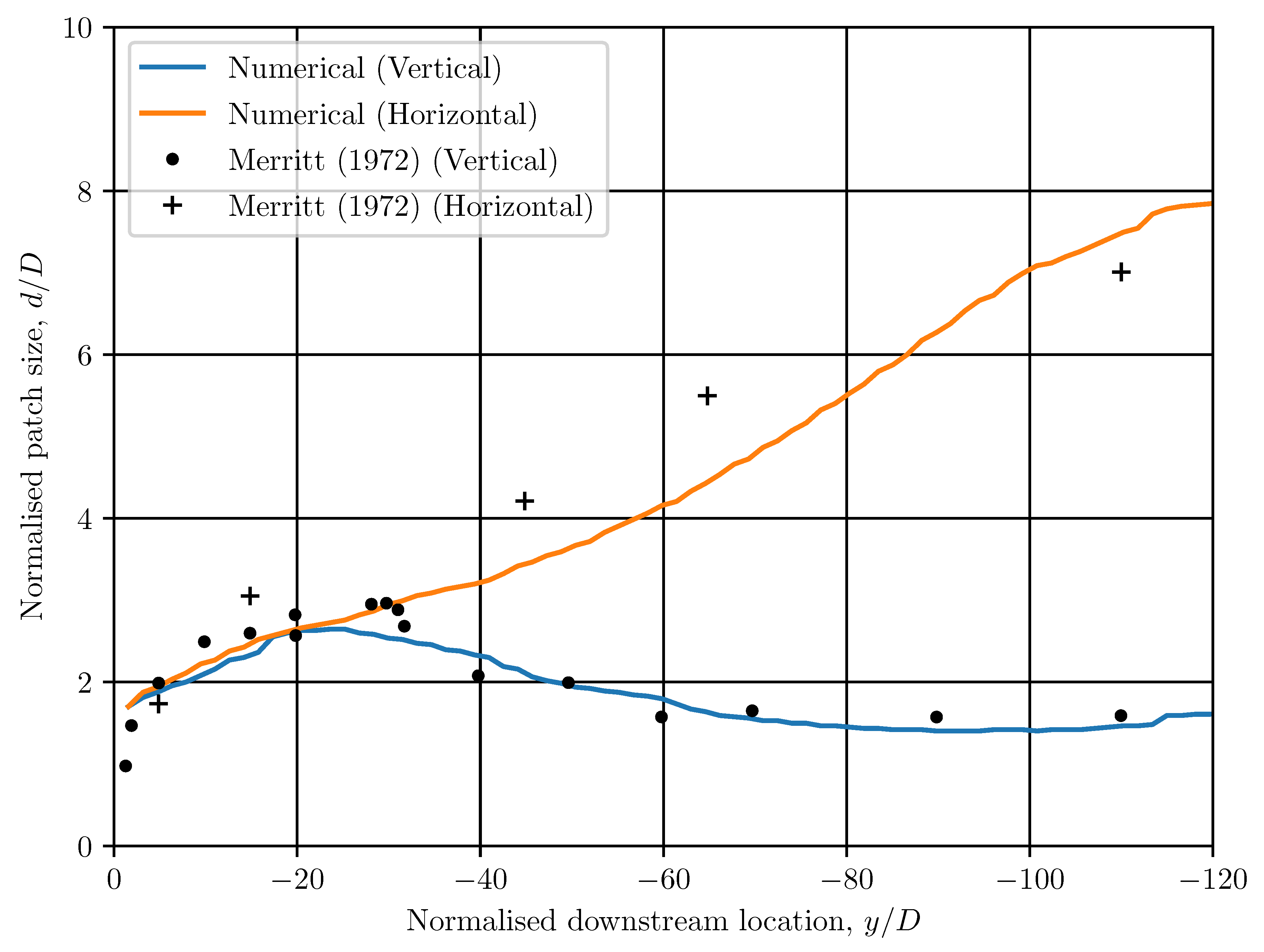
In general, the numerical model was able to capture the key stages of mixed patch evolution and yielded a qualitative agreement with the experimental observations. In order to provide a quantitative assessment of the model’s validity, the dimensions of the mixed patch were compared with data from the analogous experiment by Merritt [4]. The mixed patch’s dimensions were measured consistently by introducing several sets of probe points at various locations downstream of the propeller. The x–z plane was populated with two intersecting lines of probe points along x = 0 m and z = −0.05 m, yielding a ‘plus’ shape. As a first approximation, the vertical and horizontal extent of the mixed patch were assumed to be the distance between the outermost points (along the corresponding line of probes) at which a threshold value of 10% of $\max \left(∥u-u_0∥\right)$ was attained.

The measurements plotted in Figure 5 indicate that the mixed patch grows to approximately 2.5 times the propeller’s diameter at a distance of 20D m downstream, which is close to the expansion factor of ∼3 measured in the experiments. As the mixed patch collapses further downstream the vertical extent eventually reaches a plateau at ∼80D m as the isopycnals are restored to their original positions in the stratification. The numerical data closely agrees with the experimental data for vertical extent. However, the horizontal extent in the simulation is typically up to one propeller diameter (D) smaller than the analogous experiment. This discrepancy may have been due to the asymmetric nature of the collapse; the swirl/vorticity present in the flow may have hindered the lateral spreading along the straight line of probe points. Overall, however, this comparison with experimental data represents a successful step towards the validation of the numerical model.

Scaling Laws

Another useful validation exercise involves comparing the mixed patch’s dimensions against empirical scaling laws for height and width. It is helpful to define these scaling laws in terms of a non-dimensional buoyancy time $N{t}_e$, where $t_e$ represents the elapsed time since the mixed patch was generated (i.e., the elapsed time following the passage of the propeller). Removing the dependence on non-dimensional downstream distance ($y/D$) allows the point of mixed patch collapse to be determined without knowledge of the mixed patch’s initial diameter D. The spatial-temporal relation

$$N{t}_e=\frac{1}{\mathrm{Fr}}\frac{\left|y\right|}{D},$$

(6)

is applied in order to accomplish this. Note that the absolute value of y is considered here since downstream locations are represented by a negative value in the computational domain.

For example, a scaling law for the initial mixed patch growth stage (from $N{t}_e$ = 0 to $N{t}_e\approx$ 0.2), derived by Lin & Pao [5] by fitting to their experimental data, is given by

$$\frac{d}{D}=0.8{\mathrm{Fr}}^{0.25}{\left(N{t}_e\right)}^{0.25},$$

(7)

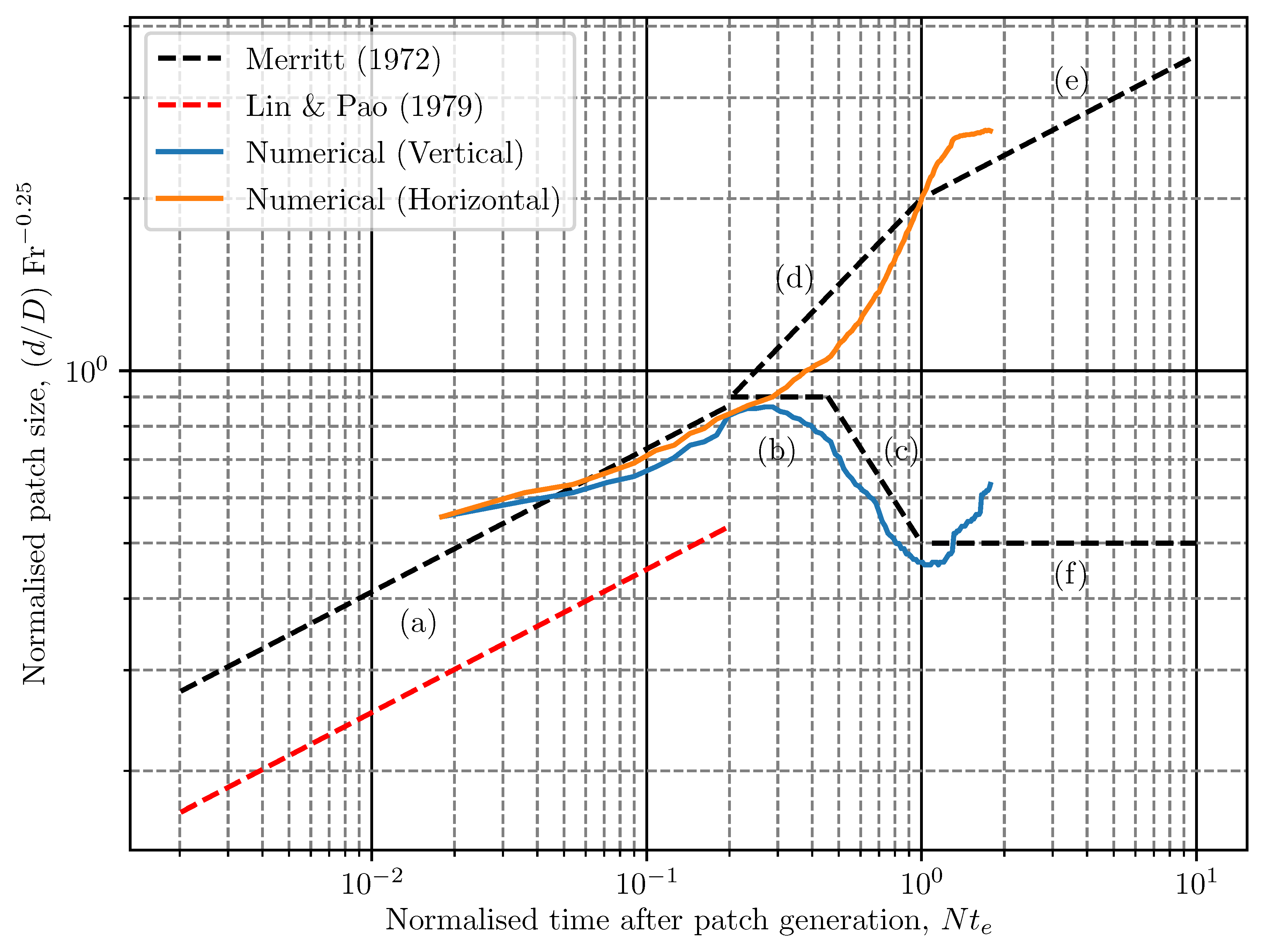
where d is the dimension of the mixed patch in either the vertical or horizontal direction. Similar scaling laws are given by Merritt [4] for each stage of the mixed patch dynamics. A plot of the numerical results in Figure 6 illustrates a generally good agreement with these scaling laws (labelled (a) to (f)).

Between $N{t}_e=0$ and $N{t}_e$ = 0.2 the expanding mixed patch in a stratification is expected to grow at a rate proportional to ${\left(N{t}_e\right)}^{0.25}$ (scaling laws in region (a)); the same rate observed for a non-stratified environment. The numerical results between $N{t}_e$ = 0.08–0.2 successfully exhibit this rate of expansion. The slower rate observed immediately downstream of the propeller (between $N{t}_e$ = 0 to 0.08) may be attributed to a lower rate of turbulent mixing by the propeller blades compared to the oscillating grid apparatus used in the experiments.

Eventually the potential energy of the enlarged mixed patch becomes equal to the turbulent kinetic energy introduced by the propeller. The mixed patch reaches a (maximum) stationary point and vertical growth ceases (b). In the numerical model this maximum occurred at $N{t}_e$ = 0.2–0.3, which concurs with the value of $N{t}_e$ = 0.23 from the empirical fit of Lin & Pao [5]. At this point, buoyancy forces start to dominate inertia, subsequently resulting in the rapid vertical collapse (c) and lateral spreading (d) of the mixed patch. The numerical results generally agree with the rate of vertical collapse. However, the rate of lateral spreading varied significantly; initial slower spreading followed by a faster spreading than the scaling law suggests. This may have been due to residual vorticity effects from the propeller’s motion.

The scaling laws at later times ($N{t}_e\ge$ 1, scaling laws (e) and (f)) suggest that the mixed patch’s thickness tends towards a vertical asymptote as the isopycnals continue to spread out post-collapse (albeit at a slower rate than the collapse stage) in order to recover the original stratification. However, it is likely that ambient internal waves generated by the collapse process cause a small amount of variation in the measured thickness as the disturbed region of fluid oscillates about its equilibrium point. This may explain the slight increase in vertical extent in the numerical results for $N{t}_e\ge$ 1.

4. Conclusions

This work successfully modelled a scaled-down KCD-32 propeller system rotating in a stratified fluid environment using the OpenFOAM modelling framework. This was accomplished by modifying the buoyantPimpleFoam solver using the DyM and AMI functionality readily available within OpenFOAM. The numerical results presented in this paper represent a successful step towards validating the numerical model. The dynamics throughout the simulation generally agree well with published experimental data and scaling laws. Any minor differences/deviations may have been caused by the significant vorticity introduced by the propeller (compared to the grid-based approaches of Merritt [4] and Lin & Pao [5]). It is worth noting that these scaling laws can potentially be validated and extended by large-scale applications or additional experiments covering a wider range of mixed patch parameters.

It is recommended that future work considers the effect of a propeller’s angle of attack on the dynamics. A non-linear stratification could also be introduced to determine the effect a strong pycnocline has on the dynamics. Furthermore, the mixed patch characteristics are known to depend on the Reynolds number of the flow [5]. The Reynolds number for the simulation presented in this paper, based on the flow speed and the diameter of the propeller, was 64. Considering a range of higher Reynolds numbers to produce strong eddies, and modelling or directly resolving the turbulence, would provide a more detailed understanding of turbulence levels in the mixed patch.