Abstract
Numerical simulations of rotating two-dimensional turbulent thermal convection on a hemisphere are presented in this paper. Previous experiments on a half soap bubble located on a heated plate have been used for studying thermal convection as well as the effects of rotation on a curved surface. Here, two different methods have been used to produce the rotation of the hemisphere: the classical rotation term added to the velocity equation, and a non-zero azimuthal velocity boundary condition. This latter method is more adapted to the soap bubble experiments. These two methods of forcing the rotation of the hemisphere induce different fluid dynamics. While the first method is classically used for describing rotating Rayleigh–Bénard convection experiments, the second method seems to be more adapted for describing rotating flows where a shear layer may be dominant. This is particularly the case where the fluid is not contained in a closed container and the rotation is imposed on only one side of it. Four different diagnostics have been used to compare the two methods: the Nusselt number, the effective computation of the convective heat flux, the velocity and temperature fluctuations root mean square (RMS) generation of vertically aligned vortex tubes (to evaluate the boundary layers) and the energy/enstrophy/temperature spectra/fluxes. We observe that the dynamics of the convective heat flux is strongly inhibited by high rotations for the two different forcing methods. Also, and contrary to classical three-dimensional rotating Rayleigh–Bénard convection experiments, almost no significant improvement of the convective heat flux has been observed when adding a rotation term in the velocity equation. However, moderate rotations induced by non-zero velocity boundary conditions induce a significant enhancement of the convective heat flux. This enhancement is closely related to the presence of a shear layer and to the thermal boundary layer just above the equator.
1. Introduction
Many atmospheric and geophysical flows are actually fluid flows on curved surfaces and can be modeled by two-dimensional thermal convection. In nature and technological applications [1], many physical phenomena are actually related to buoyancy-driven flows whether affected by background rotation or not. In particular, buoyancy driven by temperature, and affected by the rotation of the Earth, is one of the leading force in oceans [2,3,4] and atmosphere. The combined effects of rotation and buoyancy lead to the formation of large structures called cells (such as polar, Ferrel or Hadley [5] cells). Large scale flows generated by rotation and buoyancy are also observed in the outer core of the earth [6,7,8,9]. These large scale zonal flows are also observed on the Sun and other planets of our solar system [10,11]. The Rayleigh–Bénard convection model is commonly used for studying such physical phenomena. This model consists, in general, in a cylindrical convection cell on a rotating table [12,13,14,15,16,17,18,19]. Much insight about the role of rotation on such flows has been gained from such an experimental model. Other systems have been proposed to study the role of rotation on thermal convection and notably in a curved geometry which bears some relevance to atmospheric flows. A half soap bubble heated at the equator has been recently proposed in some numerical and physical experiments [20,21] to study thermal convection. Indeed, in these experiments, thermal convection and the movement of large scale structures have been observed on the surface of the bubble. The results obtained in these experiments have shown some strong similarities with atmospheric flows [20,21,22]. It has been shown in particular in these studies that the dynamics of vortices on the bubble surface and tropical cyclones [20,21,22] present the same statistical behavior. Heating on one side (the equator) is responsible for the creation of intense thermal convection leading to turbulent velocity and temperature fields whose statistical properties can be described by theories of turbulent thermal convection elaborated by Corrsin, Obukhov and Bolgiano [20,21]. Further and by subjecting the bubble to rotation, strong effects of the rotation have been observed on the nature of the fluctuations. These experiments of hemispherical bubbles heated at the equator allow to study thermal convection without the presence of lateral walls. A variety of physical phenomena of relevance to atmospheric and geophysical flows can be explored with such numerical and experimental setup.
We here consider such a hemispherical system numerically and explore two different ways for forcing the rotation of the bubble. The first method to force a rotation on a system is to add a rotation term in the mathematical model. This method is classically used in numerical simulations of rotating Rayleigh–Bénard convection where the cells (top and bottom plates, lateral walls) are submitted to a rotating force. It has also been used in our first study of rotating half soap bubble where second-order temperature structure functions have been used to compare the numerical simulations to the physical experiments [23]. However, this solid rotation does not exactly correspond to the experimental protocol where the bubble is located on a rotating table (it does not correspond to classical rotating Rayleigh–Bénard convection experiments either since, in this case, it is the boundaries, both upper and lower as well as lateral, of the container which produce the rotation of the fluid). In the experiments on rotating half soap bubbles, only the equator is subjected to the rotation force leading to the presence of a shear layer. The effects of this forcing as well as the differences with a global rotation forcing are the subject of this paper. As we will see below, the two methods affect the flow but their effects are markedly different from each other. The mathematical way to reproduce this phenomenon is to impose a non-zero azimuthal velocity at the equator. We will show in the sequel that these two different ways for forcing the half bubble into rotation, global rotation and azimuthal velocity at the equator, lead to different flow behaviors.
Even if our setup is different from the classical Rayleigh–Bénard setting, we will however compare our results with those obtained with classical rotating Raleigh–Bénard experiments. A stereographic transform, fully described in our previous papers, allows us to project the Navier–Stokes equations onto the equatorial plane. Regular Cartesian grid based methods can then be used to numerically solve the equations. The two rotation forcing models are described in Section 2 and the results are analyzed and discussed in Section 3, Section 4, Section 5 and Section 6. In these sections, we will present and discuss the effects of rotation on the Nusselt number, the convective heat flux, the temperature and velocity fluctuations, and the spectral properties.
2. Mathematical Model and Numerical Computations
We first describe the mathematical model corresponding to the non-rotating case [24]. The equations for two-dimensional thermal convection under the Boussinesq approximation [25] can be used to describe the fluid behavior which does not depend on the coordinate system:
where is the total time derivative, denotes the velocity, p the pressure, the mass density, the kinematic viscosity, the coefficient of thermal expansion, the gravity field, T the temperature of the fluid, the coefficient of thermal diffusion, F is the friction factor and S is the thermal dissipation coefficient. Unlike Rayleigh–Bénard convection, two additional terms, and , have been added in order to compensate respectively the injection of kinetic and thermal energies. As explained in [24], if the parameters F and S are kept equal to zero, an accumulation of kinetic and thermal energies leading to a numerical burst of the bubble can be observed. Indeed, in usual Rayleigh–Bénard experiments, the top plate is cooled allowing to keep a constant global averaged temperature. In the experiments on soap bubbles, we do not have a specific cooling process. Only the exchange of heat between the bubble and the surrounding air and the friction with the air stabilize experimental conditions. We have to take into consideration these interactions with the air in the numerical simulations to stabilize the computations. This is why we have to artificially remove a small part of thermal and kinetic energies in the equations. This stabilization process can be interpreted as a way to take into consideration the interaction between the bubble and the surrounding air. See [24] for more details about this stabilization process.
As mentioned in the introduction, the purpose of this paper is the study of two different methods for mathematically rotating a hemispherical cap subjected to a thermal gradient:
- Method 1: adding a rotation term in the velocity equation, where denotes the rotation vector
- Method 2: adding a non-zero azimuthal velocity boundary condition at the equator.
The equations with the rotation forcing term has to be written in a non-dimensional form. Using L, and the characteristic velocity (where denotes the difference of temperature between the pole and the equator, and L the characteristic length equal to the radius of the bubble ), the equations can be made non-dimensional. As in many papers about thermal convection, the control parameters in our numerical simulations are the Rayleigh number and the Prandtl number . Various values for the Rayleigh and Prandtl numbers have been used, but the only numerical results presented in this article are for and . We also have to define the corresponding dimensionless friction factor and the dimensionless thermal dissipation coefficient . We remind here that the goal of these dimensionless factors is to take into consideration the interaction between the bubble and the air. The empirical evaluation of their respective values has been described in [24] and we chose here , which leads to a stationary state in the non-rotating case. Using the same notation for the dimensionless pressure, velocity and temperature, the non-dimensional equations, with a rotation forcing term (Method 1), can thus be written as:
where denotes the Rossby number, the rotation rate and the vertical unit vector. Adding a rotation term in the equation is classically used for modeling rotating Rayleigh–Bénard experiments. However, method 2 best describes our physical experiment where the bubble lays on top of a rotating table. Only the part of the bubble in contact with the table is submitted to the rotation forcing thus creating a shear stress and possibly shear induced instabilities. Both methods induce a rotation of the bubble but the corresponding flows present different physical behaviors in terms of the capacity of convecting the heat flux. Four analysis tools will be used in the next parts to compare both methods:
- the Nusselt number criterion
- the convective heat flux (defined in the sequel)
- the velocity and temperature fluctuations RMS (to evaluate the shear and thermal boundary layers)
- the energy/enstrophy/temperature spectra and fluxes
Two kinds of coordinate systems are considered here: the usual 3D orthogonal Cartesian coordinates and a 2D orthogonal Cartesian coordinate system obtained by a stereographic projection onto the equatorial plane. The stereographic projection is a well known mapping allowing to project a sphere onto a plane. Usually, the projection is defined on the entire sphere, but in the present study we do not need to described the whole sphere. Thus, we use in this study a version of the stereographic projection restricted to the northern hemisphere. It can be shown that this mapping is bijective and preserves the angles. The consequences being that a Cartesian grid on the plane corresponds to a Cartesian grid on the surface of the sphere. The two kind of coordinates are related to each other by the following equalities:
and
where r denotes the radius of the sphere. Figure 1 illustrates the stereographic projection where a point P on the sphere is projected on on the equatorial plane. Using the stereographic coordinates and the calculations detailed in [24], the Navier–Stokes Equation (2) for a hemisphere of radius can thus be written using stereographic coordinates:
where are the two components of the velocity field in the stereographic coordinates. As can be noticed, the stereographic projection of the Navier–Stokes equations induced much more complicated expressions, with a couple of extra terms, compared to the usual cartesian coordinates formulation. But since the stereographic coordinates form a two-dimensional orthogonal basis, traditional numerical methods to solve the equations on cartesian grids can be used. The circular domain in the equatorial plane, a no-slip boundary condition on the equator, as well as a Dirichlet boundary condition for T are defined by using a -penalization method. This kind of method consists in adding two penalization terms: , in the temperature equation and , in the momentum equation and to consider the set of equations on the whole square domain. The boundaries are then considered like a porous medium of very low permeability [26]. In our numerical simulations, C is set equal to in the bubble, and equal to outside. The boundary conditions are then imposed by taking and for method (1) and and for method (2). When in the bubble, these extra terms vanish and we solve the regular Equation (1), and when outside the bubble, all the other terms are numerically very small compared to the extra terms except the pressure gradient. There is a coupling between these terms and the pressure gradient to yield Darcy equations and we get and at the boundary. Finite differences schemes have been chosen for solving the equations described in the previous part. A staggered uniform Cartesian grid with a mesh size , where and are the discretization steps in each direction on the projection plane, is used to discretize the spatial domain. The corresponding uniform time steps is denoted . The unsteady term in the governing equations is solved by using a second-order Gear scheme. The convection terms are solved using an explicit scheme whereas the linear terms are solved using an implicit one. If one denotes by the approximation of at time , then the approximation of the total time derivative of a general variable using the second-order Gear scheme can be written as:
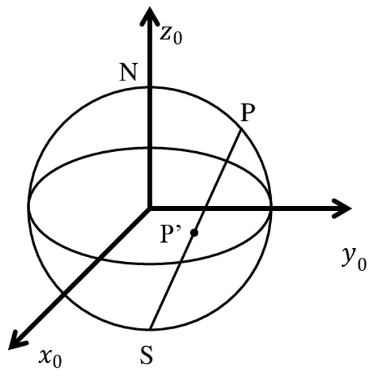
Figure 1.
Stereographic projection: the point P of coordinates on the sphere is projected on P’ of coordinates on the plane. N and S denote respectively the north and south poles. (Reproduced with permission from [24]).
As shown in Figure 2, the discrete values of the velocity field are located at the middle of the cell sides and the discrete values of the pressure p and the temperature T are located at the center of each cell. A Murman-like scheme is used for the approximation of the convection terms. This kind of scheme has been fully described in [27]. A time splitting has been used to first solve the temperature equation and then the coupled pressure and velocity equations since the temperature equation can be solved separately. A parallel process by Message Passing Interface (MPI) is used to solve both of them. A linear system of equations , where A is a pentadiagonal matrix, T is the temperature vector and E the explicit part of the discretized temperature equation is obtained by the discretization of the temperature equation. The matrix A being not a self-adjoint matrix anymore in our present curved surface problem, we have to solve this linear problem using a biconjugated gradient method. The discretization of the coupled velocity-pressure system of equations leads to solving a discrete linear system where represents the discrete operator, is the discrete equivalent of the right hand side of (8) and is the approximate solution we are looking for. All the numerical results presented in the following have been obtained with , on a grid. A grid convergence analysis in order to verify that the grid is dense enough to describe a turbulent flow had been carried out in [24]. We had computed the global temperature on the bubble for different sizes of the grid and for a given Rayleigh number. The results obtained with the grids and for various values of the Rayleigh number, and various values of the rotation rates, were almost exactly the same, whereas the results obtained with coarser grids ( and ) were slightly different. As shown in [24], a fine grid () would be better to describe the boundary layer at the equator, but would not modify the global behavior of the fluid in the bubble. The grid has thus been chosen in the present study for performing the various numerical simulations. Different values for the parameters and have been tested in [24] to stabilize the computations. The bubble can be stabilized with and which are the values used in the numerical simulations. Examples, in the non-rotating case, for the temperature and the vorticity fields are given in Figure 3 for two different times: at the beginning of the simulation (top) and in the stationary state (bottom). We can observe in Figure 3 thermal plumes emerging at the base of the bubble. The experiment is similar to a long two-dimensional toric Bénard cell in the beginning of our simulation: the cold fluid is heated from below, and the plumes are convected upward. In the beginning, there is no interaction between the plumes and the center of the domain remains empty. We can also observe these small thermal structures emerging from the heated equator on the vorticity field. The plumes continue to grow over time and start to interact with each other. As can be observed in Figure 3, the small structures along the equator are now giving birth to vortices that move along the bubble surface. A stationary state can be achieved and the results presented in the sequel have been obtained in this regime of the numerical experiments.
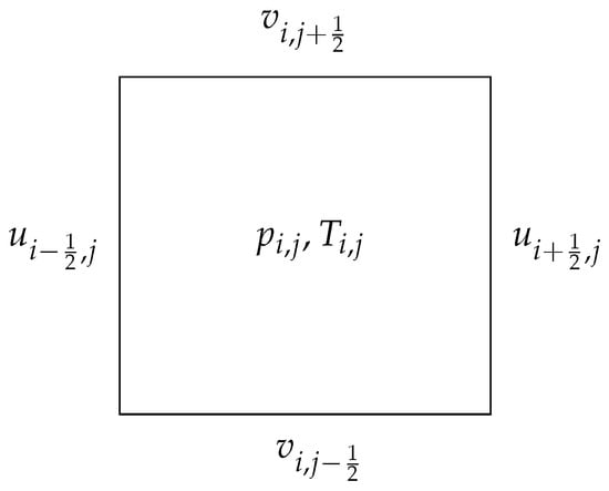
Figure 2.
Description of numerical spatial cell: the velocity components are computed in the middle of the cell borders whereas the pressure and the temperature are computed at the center of the cell. (Reproduced with permission from [24]).
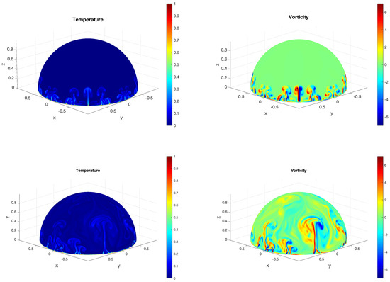
Figure 3.
Top: Beginning of the simulations; mushroom shape structures are created at the equator. Bottom: Stationary state; plumes move up on the bubble and the structures start to interact with each other. Left: Temperature fields. Right: Vorticity fields.
3. Nusselt Number Criterion
The Nusselt number is usually defined as the ratio of the total vertical heat flux and the conductive heat flux, and can be evaluated on any horizontal plane in a Rayleigh–Bénard cell. But since our experiment is not a Rayleigh–Bénard cell, we have to first define a local Nusselt number and then compute the average of all the local Nusselt numbers on the bubble. For a given latitude l, we can define the local Nusselt number as:
where denotes the vertical component of the velocity, along the vertical unit vector , T is the temperature, and stand for a temporal average in time over a latitude l. We can then obtain a global Nusselt number by averaging the local Nusselt numbers over all latitudes. In classical Rayleigh–Bénard experiments a constant heat transfer is established between the two plates and the difference between “local” vs. “global” Nusselt numbers is meaningless. In these cases, it is possible to calculate a Nusselt number by averaging over any horizontal plane. However, local and global Nusselt numbers are important physical values to evaluate when the heat transfer depends on the height, as in an open channel or in our bubble experiment (see Equations (4) and (5) in [28] for instance). The global Nusselt number has to be understood as a global indicator of the convection vs conduction balance in the cell.
Physical and numerical experiments found in the literature show that the rotation introduces three different regimes [12,14,15,16,17,18,19] in three-dimensional Rayleigh–Bénard experiments. The three regimes can be characterized using the Nusselt number. For low rotation (small and large ), the flow remains almost unaffected by the rotation. The heat transfer measured by the Nusselt number does not change in this regime and a large scale circulation is observed in the cell. For moderate rotations, the flow is affected by the rotation leading to an enhancement of the heat flux. In this regime, in 3D, the large scale circulation is replaced by vortical structures (also called plumes in the literature). The enhanced convective heat flux is directly related to the vortical structures created by the moderate rotation of the system. For high rotation, the fluid is totally dominated by the rotation forcing and the convective heat flux is decreased. The transition between the moderate and the high rotation regimes is defined in [29] as the rotation for which the Nusselt number is maximum.
In our results, we also observe three different regimes. The ratio for various values of and the ratio for various values of are reported in Figure 4. The relative Nusselt number is hardly affected for high values of Ro or small azimuthal velocities. For low values of Ro or high values of the azimuthal velocity, the relative Nusselt number decreases, showing that the flow is dominated by rotation. For intermediate values of both control parameters, the relative Nusselt number is greater than 1. As can be observed, the rotation created with the rotation forcing term (Method 1) does not significantly increase the heat flux. The maximum increase being less than 5%.
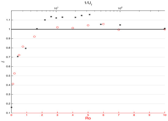
Figure 4.
Red circles: Method 1, ratio of the Nusselt number in the presence of global rotations to (no rotation). Black stars: Method 2, ratio of the Nusselt number in the presence of azimuthal velocity boundary conditions to (no rotation).
However, an increase of more than 15% is observed when the rotation is created by a moderate azimuthal velocity boundary condition (Method 2). This increase of the convective heat flux is of the same order as the one observed in the 3D rotating Rayleigh–Bénard case [12,14,15,16,17,18,19]. Note here that the Nusselt number ratio does not present a narrow maximum as in 3D experiments and simulations but a wide and plateau-like region, making it difficult to define an exact transition limit as in [29] between the regime where the Nusselt number is enhanced by rotation and the regime where the Nusselt number is decreased at high rotation rates. So we use a slightly modified definition for this transition in our study and define the three regimes by comparison to the non-rotational case as:
- Regime I where the Nusselt number is unchanged: low rotation,
- Regime II where the Nusselt number is increased: moderate rotation,
- Regime III where the Nusselt number is decreased: high rotation.
Considering the results shown in Figure 4, this definition for the transition from Regime II to Regime III seems to be more natural and better adapted for the functional shape of the variation of the relative Nusselt number versus Ro or . The structures responsible for the Nusselt enhancement in regime II will be described in the next part.
4. Convective Heat Flux
The convective heat flux, created by the buoyant forces, corresponds to the transport of heat by the movement of the fluid from hot areas (at the equator) to cold ones (north pole). In classical Rayleigh–Bénard experiments, the structures responsible for the convective heat flux are called “plumes” [13,30] and are usually characterized by a strong correlation between the temperature fluctuations (where denotes the overall time and space average) and the vertical velocity. In our numerical simulations, the vertical velocity is replaced by the radial component (pointing to the north pole) of the velocity, and the convective heat flux is then defined by where l denotes the latitude in radians. This mathematical object precisely measures the heat that is moved upward from the equator to the north pole. We obtain with our convective heat flux the same kind of information as the plumes counting described by Pieri et al. (see Figures 5 and 6 in [13]). Our results for various values of the Rossby number (Method 1) and of the velocity boundary condition (Method 2) are summarized in Figure 5.
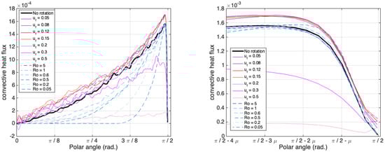
Figure 5.
Left: Convective heat flux for various values of the Rossby number and of velocity boundary condition . Right: Zoom close to the equator with .
The first striking observation is that moderate velocity rotations induced by the non-zero velocity boundary condition (Method 2) create increases of the convective heat flux at the equator, and this initial bonus of heat flux is then maintained in the bulk of the bubble. This increase is observed for all the values of for which the Nusselt number was increased ( ratio larger than 1). It can be observed that the profile of the heat flux for is the same as the profile of the heat flux without rotation confirming the result obtained with the Nusselt number criterion. Relatively strong velocity rotations in Method 2 decrease the convective heat flux at the equator leading to a decrease of the Nusselt number. This observation can be linked to our analysis about the instabilities and thermal boundary layers of the next part. Thermal plumes are created at the edge of the thermal boundary layer. When the shear layer is thinner than the thermal boundary layer then the “new born” plumes are boosted by a non-zero average velocity field. But when the shear layer limit reaches the thermal boundary layer limit, the “new born” plumes are swept by the rotations.
No increase is observed with the rotations induced by Method 1, and we even observe that the convective heat flux is strongly decreased in the bulk. Again, this result will be discussed in light of the analysis of the RMS of velocity fluctuations in the next section: high velocity rotations prevent the structures from reaching the high latitude areas. However, we can observe in the equator area (Figure 5 right) that very high velocity rotations ( for instance) induce the same kind of increase as those obtained with Method 2. But, since the global rotations also completely inhibit the dynamics in the bulk, the benefit of the increase is immediately erased as we get farther from the equator. The extra convective heat flux in the equator area is not sufficient to compensate the lack of heat flux in the bulk. Thus, the overall balance in this situation is negative and leads to a Nusselt number lower than the one obtained in the no-rotation case.
We can also visualize the plumes responsible for the convective heat flux in the convective heat fields for various values of the parameters and . In Figure 6, mushroom-shaped plumes can be observed in the non-rotating case. Short and medium sized plumes are present all around the bubble. The effects of rotation through Method 1 for can be observed in Figure 6. The long plumes have completely been suppressed and only the short plumes are present very close to the equator. Most of the surface of the bubble is now completely free of structures. In the case of Method 2, moderate velocity rotations increase the length of the plumes as can be observed in Figure 6. However, for high velocity rotations (top Figure 7), long plume structures are still present but are very localized in a small part of the bubble. For very high rotations (bottom Figure 7), very few and very localized structures can be observed almost reaching the north pole. This is a completely different phenomenon from what we can observe with a very small Rossby number in Method 1. With Method 1, the long plumes are suppressed but short plumes are still present all over the bubble. With Method 2, however, short plumes are absent and a few, localized, and weak heat structures succeed in detaching from the equator to escape to the north pole. This is a clear observation of the intermittent character of the dynamics induced by the rotations created by Method 2.
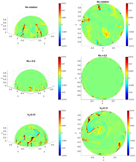
Figure 6.
Convective heat flux fields. Top: No-rotation case. Middle: Method 1 with . Bottom: Method 2 with . Left: Side view. Right: North pole view.
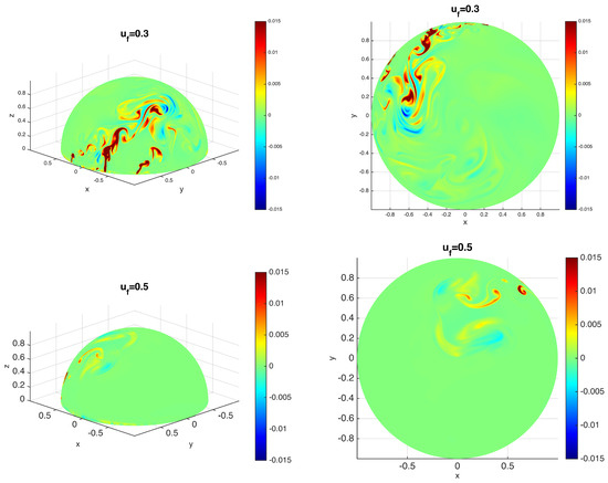
Figure 7.
Convective heat flux fields with method 2. Top: . Middle: . Left: Side view. Right: North pole view.
Even if our setup is completely different we can make a parallel with two new studies about 3D rotating Rayleigh–Bénard Convection. Rajaei et al. [31] recently published new results about the rotation dominated regime in rapidly rotating Rayleigh–Bénard convection. They found that the transition to the rotation dominated regime coincides with the suppression of vertical motions, the strong penetration of vortical plumes into the bulk and a reduced interaction of vortical plumes with their surroundings. In Alards et al. [32], the authors study in detail, with a Lagrangian approach, the transition from the rotation-unaffected regime, where the heat transfer is constant, to the rotation-affected regime, where the heat is enhanced. They found a sharp transition in the horizontal acceleration statistics near the top plane at a Rossby number lower () than the one typically found for the transition between rotation-unaffected/affected regimes (). According to their study, the steepening of the velocity gradients at the boundary and the generation of swirling convective flows in the boundary layers are two partially separate processes: heat transfer enhancement at and generation of vertically aligned vortex tubes at . They also observe a crossing between the thermal and the Ekman layers for a Rossby number equal to whereas the maximum of the Nusselt enhancement is located for between and .
5. Velocity and Temperature Fluctuations RMS
It has been shown in Section 3 that the Nusselt number is greatly influenced by the way the rotation is forced on the bubble. The difference between the two methods is that in one case the rotation is imposed on the whole bubble (Method 1 with the rotation term in the equation) whereas in the other method the rotation is imposed at the equator only (Method 2). The latter method creates a shear layer that might be responsible for the Nusselt number enhancement. So in this part, the RMS of the fluctuations of azimuthal (parallel to the equator) and radial (pointing to the north pole) velocity components are studied and compared to the thermal boundary layer (evaluated with the temperature fluctuations RMS as in [24]).
It can be noticed in Figure 8 that the rotations created by Method 1 significantly change the temperature fluctuations in the bulk of the bubble, but not so much at the equator. Indeed, in the bulk, the temperature fluctuations are suppressed by high rotation whereas close to the equator the location and the height of the maximum of the RMS is not significantly modified by the rotation forcing. This can be also observed in Figure 9 (top), where no difference can be observed in the temperature profiles at the equator, except a small increase beyond the thermal boundary layer for very high rotations.
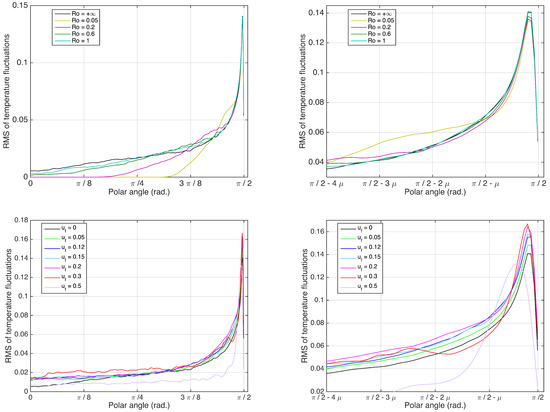
Figure 8.
Temperature fluctuations RMS. Top: Method 1 for various values of the Rossby number. Bottom: Method 2 for various values of the forcing . Right: Zoom around the equator; .
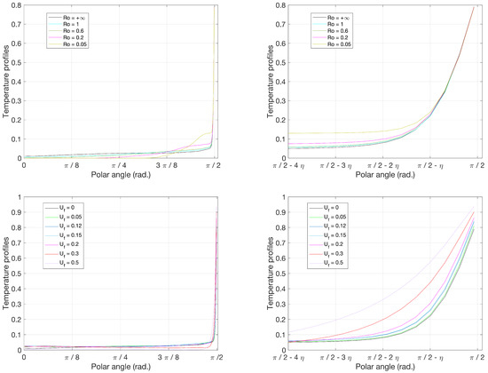
Figure 9.
Temperature profiles. Top: Method 1 for various values of the Rossby number. Bottom: Method 2 for various values of the forcing . Right: Zoom around the equator; .
From this first observation, we can conclude that the rotations induced by Method 1 do not modify the thermal boundary layer, but suppresse the temperature fluctuations in the bulk of the bubble. Let us now turn to Method 2. Moderate rotations forced by the velocity boundary condition (Method 2) slightly increase the temperature fluctuations in the bulk but significantly modify them close to the equator. Indeed, a shift of the maximum location of the RMS away from the equator can be observed. This shift is accompanied by a small increase of the maximum for moderate rotations, and a strong decrease for high rotations. The shift is also more important for large rotation velocity (bottom of Figure 8). The temperature increases at the equator can be also verified in Figure 9 (bottom) where the temperature is directly related to the rotation velocity values . So Method 1 influences the flow essentially in the bulk of the bubble while Method 2 essentially influences the thermal boundary layer which grows with the forcing velocity and which eventually also influences the bulk.
The study of the radial (pointing to the north pole) and azimuthal (parallel to the equator) velocity components fluctuations can complete this analysis.
As can be observed in Figure 10, rotations created by Method 1 significantly decrease the velocity fluctuations (both radial and azimuthal ). The size of the area where the fluctuations are the largest decreases with the increase of the rotation speed. It can also be observed that the azimuthal velocity component fluctuations present a “double bump” shape. This particular shape corresponds in fact to clockwise and counterclockwise fluctuations. This aspect can be verified by visualizing the averaged azimuthal velocity component Figure 11 (Left). We can observe three bands: close to the equator the average motion is in the same direction as the forcing (counterclockwise), then in the other direction and finally again in the same direction as the forcing. The bandwidth is decreasing as the rotation is increasing. This phenomenon, also highlighted in the soap bubble experiments, might be related to the circulation cells in the atmosphere where easterly and westerly winds are observed.
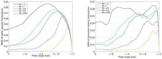
Figure 10.
Method 1. Left: Radial velocity component fluctuations RMS for various values of the Rossby number . Right: Azimuthal velocity component fluctuations RMS for various values of the Rossby number .
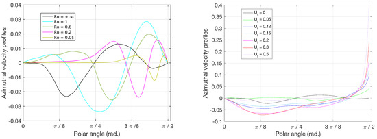
Figure 11.
Azimuthal velocity profiles. Left: Method 1 for various values of the Rossby number ; Right: Method 2 for various values of .
With Method 2, the influence of the rotation forcing on the fluid can be observed in Figure 12. Except for very large forcings ( for instance), the radial velocity component fluctuations are increased around the pole. Moderate rotations with Method 2 seem to push more fluid to the pole than the convection alone without rotation. A close look at the area above the equator (Figure 12 right) allows us to remark that the RMS profiles present a minimum when . We conjecture that this minimum corresponds in fact to the limit of a shear layer, only present with this way of rotating the bubble, and has to be compared to the limit of the thermal boundary layer (BL). The size of these two layers for various values of the rotation forcing are summarized in Figure 13. Two linear fits obtained from the first six values of , from to , are also materialized in this figure. We note a linear growth of this shear layer thickness with the velocity forcing. The slope of the linear fit for the shear layer thickness is estimated at , whereas the slope for the thermal boundary layer one is about . The shear layer thickness grows faster than the thermal layer, but we could not find any theoretical explanations for the values of these linear growth.
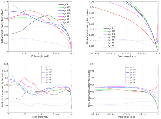
Figure 12.
Velocity fluctuations RMS for various values of (method 2). Top: Radial velocity component. Bottom: Azimuthal velocity component. Right: Zoom close to the equator; .
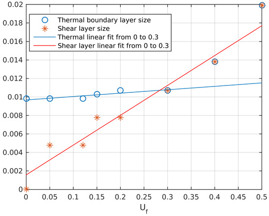
Figure 13.
Thermal boundary and shear layers sizes (polar angle in radians) for various values of the velocity forcing .
The thermal boundary layer size increases slowly while the shear layer size increases faster. When the size of this shear layer reaches the size of the thermal boundary layer near both keep the same size and continue to grow with increasing forcing velocity . This observation might be related to the phenomenon discussed in the previous part: the Nusselt number increases for moderate velocity rotations up to . As long as the shear layer size is smaller than the thermal boundary layer size the convective heat flux is enhanced by the rotation forcing, leading to an enhancement of the Nusselt number. But when the shear layer is the same size as the thermal boundary layer then the enhancement is stopped, and the Nusselt number starts to decrease.
This kind of competition between different characteristic scales has been also observed in three-dimensional Rayleigh–Bénard numerical experiments in [29,33,34] in the context of the transition between a regime where the heat transfer is not significantly affected by rotation and a rotationally controlled regime. In the non-rotationally affected regime, Rajaei observed that the kinematic boundary layer thickness remains constant and then starts to decrease when the rotation dominates the dynamics (see Figure 3.4 in [29]). This transition corresponds to a transition from a Prandtl–Blasius type layer to an Ekman type layer. The boundary layer related to the low velocity rotation regime (where they observe a Large Scale Circulation) is of Prandtl–Blasius type and the one related to the moderate velocity rotations regime is of Ekman type. Other observations were provided by King et al. [33] (see in particular Figure 3b) who found that the transition from non-rotating to rotationally controlled heat transfer occurs when the thermal boundary layer and the Ekman layer thicknesses are crossing each other.
Our observations show that for the transition between our Regime II and our Regime III, the thickness of this shear layer (found with Method 2 only) becomes comparable to the thickness of the thermal boundary layer. In fact, this transition corresponds to the progressive disappearance of the thermal plumes described in the previous part. Also, compared to Method 1, we do not observe the “double bumps” in the azimuthal velocity component RMS which was related to circulation cells. This can be also verified in the azimuthal velocity profiles in Figure 11 (right) where we do not find the caracteristic three bands. This phenomenon seems thus to be a consequence of the global rotation of the system like in the Earth’s system, and cannot be reproduced with Method 2. Also in Figure 11 (right), we can clearly observe that the azimuthal velocity at the equator is directly linked to the forcing value . In short, in the context of our two-dimensional numerical experiments, the convective heat enhancement (measured by the Nusselt number) can be produced by Method 2. Method 1 can produce a very small enhancement of the Nusselt number (less than 5%). Large circulations, detected in the azimuthal velocity component, can be produced with Method 1 but not with Method 2. As it will be shown in the next part, more insight into the dynamics of the flow can be obtained using global physical properties like spectra and fluxes.
6. Spectra and Fluxes
Energy, enstrophy and temperature spectra/fluxes are commonly used to study two or three-dimensional turbulence as well as Rayleigh–Bénard convection cells. Indeed, according to the corresponding theories, it is well known that inverse or direct cascades of energy/enstrophy in 2D or 3D turbulence or the presence of a Bolgiano–Obukhov regime in Rayleigh–Bénard convection can be detected using energy/enstrophy/temperature spectra and fluxes [24]. Very recently, Sharma et al. [35,36] published new results on rapidly rotating forced and decaying turbulence. Their studies are based on numerical simulations in a cube of size with periodic boundary conditions on all the sides. In the decaying case, they observed that the turbulent flow evolves in time with a real Rossby number decreasing to ∼10 and the flow becoming quasi two-dimensional with strong coherent columnar structures arising due to the inverse cascade of energy (as in classical two-dimensional turbulence where strong vortices are observed). They propose a new scaling for the energy spectrum of three-dimensional rapidly decaying turbulence: , where is the enstrophy dissipation rate, the enstrophy dissipation number, and C a positive real constant. For the rapidly rotating forced turbulence, they propose a scaling split into two components related to the horizontal plane and the vertical rotation axis in the range of wavenumbers smaller than the forcing scale: where ⊥ and ‖ denote the directions perpendicular and parallel to the vertical rotation axis. However, our numerical setup being different, and our rotation speed being weaker, we cannot expect to obtain the same results.
Mathematical tools specifically designed for spherical problems has to be used to obtain global properties, such as spectra or fluxes, for our numerical simulations. The definitions of the spherical harmonics decomposition are first recalled and then used to compute these various physical indicators (spectra and fluxes) of interest.
Any function f with spherical symmetry can be easily written as a linear combination of special functions ,
the so-called spherical harmonics defined by:
Here, denotes the associated Legendre polynomials. The expansion coefficients are then obtained by projection of f onto the spherical harmonics:
The integration over is actually a Fourier transform and is numerically computed with a traditional routine. The power spectrum can then be computed from the coefficients :
The coefficients are thus equivalent to the Fourier coefficients and the coefficients are equivalent to the Fourier wavenumbers in a traditional Fourier power spectrum. For instance, the thermal energy is defined as:
where
Energy, enstrophy and thermal fluxes can be also computed using the spherical harmonics coefficients. The energy flux is usually computed in the Fourier domain from the nonlinear term in the Navier–Stokes equation:
where is the nonlinear energy transfer function and is obtained by angular integration of . Here, the symbol denotes the usual Fourier transform. The enstrophy and thermal fluxes are obtained in the same way:
where and are the enstrophy and thermal transfer functions. They are obtained by angular integration of and .
So, in our study, we replace the usual Fourier decompositions by spherical harmonics decompositions, and the angular integration of the Fourier coefficients by a summation of the spherical coefficients over the degree to . The results are strictly equivalent to classical energy, enstrophy and thermal fluxes and can be considered as such.
Energy, enstrophy and temperature spectra and fluxes are given in three separate Figure 14, Figure 15 and Figure 16 for relatively strong ( and ), moderate ( and ) and no rotations. The values for relatively strong rotations are those leading to 80% of the initial (without rotation) Nusselt number, and the values for moderate rotations are those leading to the highest enhancement of the Nusselt number.
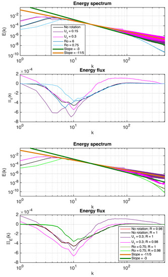
Figure 14.
First and second rows: Energy spectra and fluxes for strong, moderate and no rotation for methods 1 and 2. Third and fourth rows: Tukey windowed energy spectra and fluxes for strong rotations. Method 1 with . Method 2 with . Radius of the window .
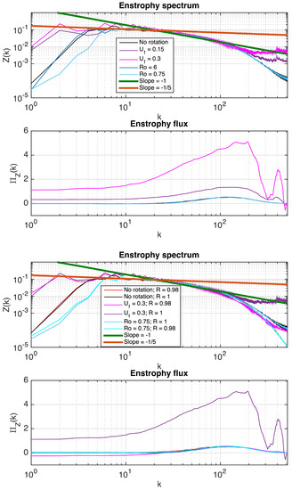
Figure 15.
First and second rows: Enstrophy spectra and fluxes for strong, moderate and no rotation for methods 1 and 2. Third and fourth rows: Tukey windowed enstrophy spectra and fluxes for strong rotations. Method 1 . Method 2 . Radius of the window .
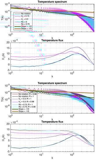
Figure 16.
First and second rows: Temperature spectra and fluxes for strong, moderate and no rotation for methods 1 and 2. Third and fourth rows: Tukey windowed temperature spectra and fluxes for strong rotations. Method 1 . Method 2 . Radius of the window .
6.1. Energy Spectra and Fluxes
The first observation is that the energy spectra corresponding to the rotating bubbles are above the spectrum of the non-rotating one at large and small scales (except at large scales for the case . As previously noticed, strong rotations with Method 1 prevent large structures to develop towards the pole). One can also notice that the slope of the energy spectrum (observed for moderate wave numbers) is not modified by the rotations. Rotations created by Method 2 induce an energy increase at large scales. The third observation concerns the small scales. Rotations created by Method 1 do not modify the energy spectrum at small scales whereas strong oscillations are detected for rotations created by Method 2. This pattern had been previously observed in temperature spectra and it had been proven that it is due to the boundary conditions at the equator [24]. These oscillations in the energy spectra are due to the non-zero velocity boundary condition. What we observe here is that Method 2 intensifies the shear layer and now the energy spectrum is also affected by these instabilities. These oscillations can be removed by excluding the shear layer above the equator from the computations. This can be done by using a circular version of a Tukey window [37] to smoothly remove the shear layer without introducing spurious artifacts. We recall here that a Tukey window allows to smooth a step from 1 to 0 with a cosine function shape decrease. We present in bottom of Figure 14 the effects of this windowing process on the energy spectra and fluxes for the strong rotations cases ( and ). The windowed and non-windowed non-rotating cases are also shown in this figure. The radius from which the window decreases has been chosen equal to . Even if it is a very short window, it still allows to significantly reduce the oscillations. It had been shown in [37] that a larger window would allow to completely remove them. As expected, the windowing process affects particularly the results obtained with Method 2 where a strong shear layer is present whereas it does not significantly modify the results obtained with Method 1 where there are kinematic and thermal layers but almost no shear layer.
In our previous paper, we have shown that, in absence of rotation, as the Rayleigh number increases, the energy (resp. enstrophy) spectra tend to follow a (resp. ) scaling corresponding to the Bolgiano regime [38,39,40,41]. Our results were consistent with Verma et al. [40] and Kumar et al. [41] confirming the two-dimensional nature of our experiment with a strong kinetic energy inverse cascade. In our present numerical simulations with an intermediate Rayleigh number () we observe a slope at intermediate scale, and the rotations created with method 2 tend to strengthen the buoyancy and a slope is observed. Particularly at large scales. The shape of the energy fluxes remains essentially the same, and we can observe that the strongest inverse energy transfer correspond to the highest Nusselt number enhancement. Strong rotations created by Method 1 lead to a weaker energy flux.
6.2. Enstrophy Spectra and Fluxes
We can observe in the enstrophy spectra that strong rotations created by Method 1 decrease the quantity of enstrophy at large scales whereas strong or moderate rotations created by Method 2 increase the quantity of enstrophy in this range of scales (first and second rows of Figure 15). This can be explained by the fact that in Method 2 very long structures stretching from the equator to the pole appear in the bubble, while Method 1 rotations pack the structures in a band above the equator. The size of this band depends on the rotation velocity. As already observed in the energy spectra, the rotations created with Method 2 strengthen the buoyancy and enable a Bolgiano regime at large scales where a can be observed. At intermediate scales, a Kraichnan-like regime with a slope takes place. As mentioned above, the rotations created with Method 1 weaken the buoyancy at large scales.
We can also observe in Figure 15 that Method 2 substantially modifies the enstrophy flux in the bubble. Method 1 does not really change the enstrophy flux, but Method 2 strongly increases it. In particular, it can be noticed the appearance of a bump at small scales around . The higher the azimuthal velocity, the higher the bump. We believe that this bump is created by instabilities in the shear layer, and can be removed by excluding the shear layer above the equator from the computations. Again, this can be done by using the circular version of a Tukey window [37] to smoothly remove the shear layer without introducing spurious artifacts. We present in Figure 15 (third and fourth rows) the effects of this windowing process on the enstrophy spectra and fluxes for the strong rotations cases ( and ). The non-rotating non-windowed case is also shown in this figure. The size of the window has been chosen as . The windowing process does not significantly change the enstrophy spectra at large scales. But we can verify that the instabilities in the shear layer are responsible for the shape of the spectrum at very small scales (in particular for Method 2). The difference is even more striking in the enstrophy flux. We can observe that the small shear layer is influencing the whole flux, and is in particular responsible for the bump located at . If we remove from the figure the flux obtained with , we can zoom and observe that the remaining fluxes are very similar at small scales (Figure 17). It can be noticed that concerning Method 1 the windowed enstrophy flux is very similar to the windowed non-rotating enstrophy flux. Even in the non-rotating case the boundary layer plays an important role in the transfer of enstrophy through scales. Thus we can conclude that the shear layer is really dominant in our experiments, for both methods of rotation, but in particular when rotating the bubble with Method 2.
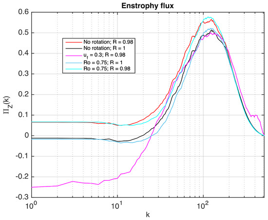
Figure 17.
Tukey windowed enstrophy fluxes for strong rotations. Method 1 . Method 2 with radius of the window only.
6.3. Temperature Spectra and Fluxes
The temperature spectra are composed of two branches leading to an oscillatory behavior. This characteristic feature has been studied and explained in detail in [24]. It was shown that the temperature spectrum presents dual branches because the mean temperature profile has a steep variation near the equator. These oscillations can be removed by subtracting the average temperature profile from the temperature fields.
Here, we observe that the rotations created by Method 1 do not significantly modify the temperature spectrum, whereas the rotations created by Method 2 largely increase the oscillations, in particular at small scales. This is consistent with our previous results since rotations induced by Method 2 strengthen the instabilities in the shear layer and thus enhance its influence in the fluid. Without rotation, we can observe a scaling in the temperature spectrum. This scaling changes slightly with rotation values and a for strong rotation with Method 2 () is observed. We do not have any explanation for theses results. We can observe in the temperature fluxes that the rotation leading to the highest enhancement of the Nusselt number (for ) has the highest temperature flux. Once again the influence of the instabilities in the shear layer can be studied by removing them with the Tukey windowing process. The results are summarized in Figure 16 (third and fourth rows). Again, removing the shear layer allows to reduce the oscillations as observed in [24]. However, here we just remove a very small area above the equator whereas in [24] the average profile of temperature was removed. We can also observe that the windowing significantly modifies the temperature fluxes in the non-rotating case and also in the case of the rotation induced by Method 1. The effect is actually the same for both cases.
In conclusion, we observe a mix of the Bolgiano and Kraichnan regimes. The rotations created by Method 2 strengthen the buoyancy at large scales and the Bolgiano regime seems to be dominant in this range of scales. This is particularly observed in the enstrophy spectra where a slope is detected in the results for Method 2. Also, two characteristics seem to play a very important role: the boundary layers that clearly influence the whole flow, and the intermittency induced by the shear layer in Method 2. Different physical mechanisms can be responsible for these phenomena and can be different in two and three-dimensional thermal turbulence: for instance, tubes of vorticity can clearly not be produced in two-dimensional experiments. However, plumes of convective heat can still be produced in two-dimensional experiments.
7. Conclusions
We have presented numerical simulations of a rotating thermal convection experiment. The results for the non-rotating version of this experiment have been reported in [20,21,22,24]. The purpose of the present paper was to analyze the reaction of the fluid when two different kinds of rotation are applied to the bubble: a solid rotation forced by a rotation term in the equations (Method 1), and a global rotation forced by a non-zero azimuthal velocity boundary condition at the equator (Method 2). The second-order temperature structure functions have already been analyzed in [23] for a rotating bubble with Method 1 for various values of the Rossby number. Three different regimes were observed in the temperature structure functions depending on the Rossby number. We have also found in the present study three different regimes when analyzing the convective heat transfer: regime I when the Nusselt number is unchanged, regime II when the Nusselt number is increased, and regime III when the Nusselt number is decreased. Three-dimensional Rayleigh–Bénard experiments also present three different regimes depending on the Rossby number [12,14,15,16,17,18,19]. In our numerical simulations, when the velocity is low (Regime I), the fluid remains unaffected and we do not observe any increase of the heat transfer. For moderate velocity rotations (Regime II), the convective heat transfer from the equator to the north pole is improved by about 5% with Method 1 and more than 15% with Method 2. For relatively high rotations (Regime III), we observe a large drop in the heat transfer efficiency with both methods. These numerical simulations have been analyzed with four different tools: the Nusselt number, the convective heat flux, the RMS of velocity and temperature fluctuations, and the energy/enstrophy/temperature spectra/fluxes. The enhancement of the heat transfer, measured by the Nusselt number, is created by the elongation of the plumes that stretch from the equator to the north pole for moderate rotations. These plumes are completely suppressed by high rotations induced by Method 1 and strongly inhibited by high rotations induced by Method 2. Rotations induced by Method 2 create a shear layer with strong velocity fluctuations near the equator.
We have shown that the Nusselt number enhancement is controlled by the relative thicknesses of the thermal and shear layers, in the same way as in [33] where they compare the thermal and the viscous layers. When the thermal boundary layer is larger than the shear layer, the heat transfer is enhanced by the rotation and we observe an increase of 15–18% of the Nusselt number compared to the non-rotating case (Regime II). When the thickness of the shear layer reaches that of the thermal boundary layer, the creation of the plumes is affected by the rotation and we observe shorter plumes in the bulk of the bubble. With Method 2, when the velocity rotation is relatively high, most of the plumes are suppressed but intermittent and rare very long structures that stretch from the equator to the pole are present. In this case, the dynamics of the fluid is completely modified and the global Nusselt number is decreased compared to the non-rotating one. The analysis of the energy/enstrophy/temperature spectra and fluxes also confirms that the small shear layer, strengthened by high azimuthal velocity rotations, plays a very important role in the statistical properties of the bubble. This method for producing the rotations strengthens the buoyancy leading to a Bolgiano-like scaling at large scales. At intermediate scales, a Kraichnan-like scaling is observed in the energy and enstrophy spectra. We also observe a dominant inverse cascade of energy and a dominant direct cascade of enstrophy.
Author Contributions
Conceptualization, methodology, validation, writing–original draft preparation, writing–review and editing, project administration, funding acquisition: P.F., C.-H.B., H.K. Software: P.F., C.-H.B. All authors have read and agreed to the published version of the manuscript.
Funding
Numerical experiments presented in this paper were carried out using the PlaFRIM experimental testbed, supported by Inria, CNRS (LABRI and IMB), Université de Bordeaux, Bordeaux INP and Conseil Régional d’Aquitaine (see https://www.plafrim.fr/). H.K. thanks the Institut Universitaire de France for partial support.
Acknowledgments
The authors wish to thank the editor and the referee for their valuable comments and suggestions.
Conflicts of Interest
The authors declare no conflict of interest.
References
- Verma, M. Physics of Buoyant Flows: From Instabilities to Turbulence; World Scientific: Singapore, 2018. [Google Scholar]
- Gascard, J.; Watson, A.; Messias, M.; Olsson, K.; Johannessen, T.; Simonsen, K. Long-lived vortices as a mode of deep ventilation in the Greenland Sea. Nature 2002, 416, 525–527. [Google Scholar] [CrossRef] [PubMed]
- Marshall, J.; Schott, F. Open-ocean convection: Observation, theory, and models. Rev. Geophys. 1999, 37, 1–64. [Google Scholar] [CrossRef]
- Wadhams, P.; Holfort, J.; Hansen, E.; Wilkinson, J. A deep convective chimney in the winter Greenland Sea. Geophys. Res. Lett. 2002, 29, 76-1–76-4. [Google Scholar] [CrossRef]
- Hadley, G. Concerning the cause of the general trade-winds. Philos. Trans. R. Soc. Lond. 1735, 39, 58–62. [Google Scholar]
- Cardin, P.; Olson, P. Chaotic thermal convection in a rapidly rotating spherical shell: Consequences for flow in the outer core. Phys. Earth Planet. Inter. 1994, 82, 235–259. [Google Scholar] [CrossRef]
- Glatzmaier, G.; Coe, R.; Hongre, L.; Roberts, P. The role of the Earth mantle in controlling the frequency of geomagnetic reversals. Phys. Earth Planet. Inter. 1999, 401, 885–890. [Google Scholar]
- Jones, C. Convection-driven geodynamo models. Philos. Trans. R. Soc. Lond. Ser. A Math. Phys. Eng. Sci. 2000, 358, 873–897. [Google Scholar] [CrossRef]
- Sarson, G. Reversal models from dynamo calculations. Phil. Trans. R. Soc. Lond. A 2000, 358, 921–942. [Google Scholar] [CrossRef]
- Heimpel, M.; Aurnou, J. Turbulent convection in rapidly rotating spherical shells: A model for equatorial and high latitude jets on Jupiter and Saturn. Icarus 2007, 187, 540–557. [Google Scholar] [CrossRef]
- Ingersoll, A. Atmospheric dynamics of the outer planets. Science 1990, 248, 308–316. [Google Scholar] [CrossRef]
- Kooij, G.; Botchev, M.; Geurts, B. Direct numerical simulation of Nusselt number scaling in rotating Rayleigh-Bénard convection. Int. J. Heat Fluid Flow 2015, 55, 1363–1367. [Google Scholar] [CrossRef]
- Pieri, A.; Falasca, F.; von Hardenberg, J.; Provenzale, A. Plume dynamics in rotating Rayleigh-Bénard convection. Phys. Lett. A 2016, 380, 26–33. [Google Scholar] [CrossRef]
- Zhong, J.Q.; Stevens, J.; Clercx, H.; Verzicco, R.; Lohse, D.; Ahlers, G. Prandtl-, Rayleigh-, and Rossby-number dependance of heat transport in turbulent rotatting Rayleigh-Bénard convection. Phys. Rev. Lett. 2009, 102, 044502. [Google Scholar] [CrossRef] [PubMed]
- Kunnen, R.; Clercx, H.; Geurts, B. Breakdown of large-scale circulation in turbulent rotating convection. Europhys. Lett. 2008, 84, 24001. [Google Scholar] [CrossRef]
- Stevens, J.; Clercx, H.; Lohse, D. Boundary layers in rotating weakly turbulent Rayleigh-Bénard convection. Phys. Fluids 2010, 22, 085103. [Google Scholar] [CrossRef]
- Rajaei, H.; Joshi, P.; Alards, K.; Kunnen, R.; Toschi, F.; Clercx, H. Transitions in turbulent rotating convection: A Lagrangian perspective. Phys. Rev. E 2016, 93, 043129. [Google Scholar] [CrossRef]
- Rajaei, H.; Joshi, P.; Kunnen, R.; Clercx, H. Flow anisotropy in rotating buoyancy-driven turbulence. Phys. Rev. Fluids 2016, 1, 044403. [Google Scholar] [CrossRef]
- Rajaei, H.; Kunnen, R.; Clercx, H. Exploring the geostrophic regime of rapidly rotating convection with experiments. Phys. Fluids 2017, 29, 045105. [Google Scholar] [CrossRef]
- Seychelles, F.; Amarouchene, Y.; Bessafi, M.; Kellay, H. Thermal Convection and Emergence of Isolated Vortices in Soap Bubbles. Phys. Rev. Lett. 2008, 100, 144501. [Google Scholar] [CrossRef]
- Seychelles, F.; Ingremeau, F.; Pradere, C.; Kellay, H. From Intermittent to Nonintermittent Behavior in Two Dimensional Thermal Convection in a Soap Bubble. Phys. Rev. Lett. 2010, 105, 264502. [Google Scholar] [CrossRef] [PubMed]
- Meuel, T.; Xiong, Y.L.; Fischer, P.; Bruneau, C.H.; Bessafi, M.; Kellay, H. Intensity of vortices: From soap bubbles to hurricanes. Sci. Rep. 2013, 3, 3455. [Google Scholar] [CrossRef] [PubMed]
- Meuel, T.; Coudert, M.; Bruneau, C.H.; Fischer, P.; Kellay, H. Effects of rotation on temperature fluctuations in turbulent thermal convection on a hemisphere. Sci. Rep. 2018, 8, 16513. [Google Scholar] [CrossRef] [PubMed]
- Bruneau, C.H.; Fischer, P.; Xiong, Y.L.; Kellay, H. Numerical simulations of thermal convection on a hemisphere. Phys. Rev. Fluids 2018, 3, 043502. [Google Scholar] [CrossRef]
- Boussinesq, J. Théorie Analytique de la Chaleur Mise en Harmonie Avec la Thermodynamique et Avec La Théorie Mécanique de la Lumière; Gauthier-Villars: Paris, France, 1903. [Google Scholar]
- Angot, P.; Bruneau, C.H.; Fabrie, P. A penalization method to take into account obstacles in incompressible viscous flow. Numer. Math. 1999, 81, 497–520. [Google Scholar] [CrossRef]
- Bruneau, C.; Saad, M. The 2D lid-driven cavity problem revisited. Comput. Fluids 2006, 35, 326–348. [Google Scholar] [CrossRef]
- Sanvicente, E.; Giroux-Julien, S.; Menezo, C.; Bouia, H. Transitional natural convection flow and heat transfer in an open channel. Int. J. Therm. Sci. 2013, 63, 87–104. [Google Scholar] [CrossRef]
- Rajaei, H. Rotating Rayleigh-Bénard Convection. Ph.D. Thesis, Technische Universiteit, Eindhoven, The Netherlands, 2017. [Google Scholar]
- Vincent, A.; Yuen, D. Plumes and waves in two-dimensional turbulent thermal convection. Phys. Rev. E 1999, 60, 2957–2963. [Google Scholar] [CrossRef]
- Rajaei, H.; Alards, K.; Kunnen, R.; Clercx, H. Velocity and acceleration statistics in rapidly rotating Rayleigh-Bénard convection. J. Fluid Mech. 2018, 857, 374–397. [Google Scholar] [CrossRef]
- Alards, K.M.J.; Kunnen, R.P.J.; Stevens, R.J.A.M.; Lohse, D.; Toschi, F.; Clercx, H.J.H. Sharp transitions in rotating turbulent convection: Lagrangian acceleration statistics reveal a second critical Rossby number. Phys. Rev. Fluids 2019, 4, 074601. [Google Scholar] [CrossRef]
- King, E.; Stellmach, S.; Noir, J.; Hansen, U.; Aurnou, J. Boundary layer control of rotating convection systems. Nature 2009, 457, 301–304. [Google Scholar] [CrossRef]
- Ecke, R.; Niemela, J. Heat Transport in the Geostrophic Regime of Rotating Rayleigh-Bénard Convection. Phys. Rev. Lett. 2014, 113, 114301. [Google Scholar] [CrossRef] [PubMed]
- Sharma, M.; Kumar, A.; Verma, M.; Chakraborty, S. Statistical features of rapidly rotating decaying turbulence: Enstrophy and energy spectra and coherent structures. Phys. Fluids 2018, 30, 045103. [Google Scholar] [CrossRef]
- Sharma, M.; Verma, M.; Chakraborty, S. On the energy spectrum of rapidly rotating forced turbulence. Phys. Fluids 2018, 30, 115102. [Google Scholar] [CrossRef]
- Bruneau, C.; Fischer, P. Spectra and filtering: A clarification. Int. J. Wavelets Multiresolut. Inf. Process. 2007, 5, 465–483. [Google Scholar] [CrossRef]
- Bolgiano, R. Turbulent spectra in a stably stratified atmosphere. J. Geophys. Res. 1959, 71, 2226–2229. [Google Scholar] [CrossRef]
- Bolgiano, R. Structure of turbulence in stratified media. J. Geophys. Res. 1962, 67, 3015–3023. [Google Scholar] [CrossRef]
- Verma, M.; Kumar, A.; Pandey, A. Phenomenology of buoyancy-driven turbulence: Recent results. New J. Phys. 2017, 19, 025012. [Google Scholar] [CrossRef]
- Kumar, A.; Chatterjee, A.; Verma, M. Energy spectrum of buoyancy-driven turbulence. Phys. Rev. E 2014, 90, 023016. [Google Scholar] [CrossRef]


Publisher’s Note: MDPI stays neutral with regard to jurisdictional claims in published maps and institutional affiliations. |
© 2020 by the authors. Licensee MDPI, Basel, Switzerland. This article is an open access article distributed under the terms and conditions of the Creative Commons Attribution (CC BY) license (http://creativecommons.org/licenses/by/4.0/).