Abstract
The present study investigates cold air recirculation in the evaporators of large-scale air-source heat pumps. A case study considered a 5 MW air-source heat pump producing heat for district heating. The heat pump comprises 20 horizontal evaporators, where each evaporator is equipped with eight fans. The evaporators were implemented in a CFD model, where the influence of the outdoor wind direction on the recirculation was investigated. Firstly, the air recirculation was analysed with no surrounding obstacles. Secondly, the surrounding building and the real ground topology was included in the CFD model, to analyse their influence on the air recirculation. The results show that recirculation occurs for all wind directions, due to the turbulent behaviour of the flow around the evaporators. The results also show that the presence of a building intensifies the recirculation when it is placed directly upstream of the evaporators due to the presence of vortices in the wake of the building. On the other hand, a ground depression helps to reduce the recirculation by having additional energy dissipation due to the sudden change in the ground direction.
1. Introduction
Large-scale heat pumps for district heating have been identified as an important technology in the green transition of the heating sector in Europe [1]. The goal of the long-term Danish energy policy is to reach a fossil fuel-free society by 2050 and to produce heat and electricity exclusively from sustainable energy resources by 2035. In 2020, district heating supplied heat to 64% of all households in Denmark, and of this, 51% came from renewable sources [2].
Large-scale heat pumps use electricity while producing heat and may therefore act as a link between the heating and electricity sector, and by using thermal storages, the heat production may be decoupled from the electricity production. Several studies show a large potential for the integration of large-scale heat pumps into the future energy system [3,4]. Lund et al. [3] conclude that in Denmark there is a potential for implementing heat pumps between 2 GW and 4 GW thermal capacity.
Heat pumps convert a low-temperature heat source into heat at the desired temperature level by using electricity. Considering a heat pump with a heating coefficient of performance (COP) of four, the heat pump requires roughly three units of energy input from a low-temperature heat source for every unit of electricity used for upgrading the heat to the desired temperature. Having in mind the large heat pump capacities, which are suggested for implementation in the future, this also means that considerable amounts of energy from the low-temperature heat sources have to be available.
The use of ambient air as a heat source in large-scale heat pumps has the great advantage of ambient air being available and accessible almost everywhere. However, several factors still challenge the deployment of large-scale air-source heat pumps (ASHPs), such as noise from the fans of the evaporators and the exhaust of cold air to the neighbourhood of the ASHP.
Another key parameter affecting the performance of an ASHP is the recirculation of cold air around the evaporator. A high recirculation can lead to a severe reduction in the heat pump COP, due to the lowered mean inlet temperature. The study of the placement of the evaporators in the environment of the ASHP will help the heat pump designers to estimate the reduction in the average inlet temperature. Consequently, a penalty factor for the inlet temperature can be introduced in a detailed model of the heat pump cycle, to take into account the air recirculation. Therefore, the influence of the wind direction and the effect of the field topology around the evaporators have to be investigated, to quantify the effect of the cold air recirculation on the performances of the ASHP.
To the authors’ best knowledge, there are very limited resources on the air recirculation of air-source evaporators used in a large-scale heat pump system. On the other hand, there have been numerous studies focusing on the plume recirculation of air cooled condensers used in power plants. Considering the air side of the heat exchangers, the functioning of evaporators and condensers is very similar. The ambient air is entrained in the heat exchanger of the condenser or the evaporator by external fans and is used as a heat source or heat sink. Therefore, the plume recirculation of condensers can be used as a reference for further study on the cold air recirculation of evaporators. Kröger [5] analysed the plume recirculation for horizontal condensers, where fans of the condensers lift the ambient air. Kröger showed that part of the warmer air recirculates back to the inlet of the fans, resulting in a lower heat transfer rate of the condenser. Duvenhage et al. [6] studied the plume recirculation for horizontal condensers using computational fluid dynamics (CFD) in two dimensions (2D). They included the effect of an incoming wind, for two different directions: longitudinal wind and crosswind. They found out that longitudinal wind increases the plume air recirculation on the lateral fans of the condenser, whereas the crosswind reduces the air volume flow rate delivered by the upwind fans. Roger et al. [7] performed similar CFD simulations in three dimensions (3D). They also included the buildings and obstacles surrounding the condensers to analyse the effect of the actual field topology on the recirculation. The results of the CFD simulations agree well when compared with on-field experimental tests, with a low deviation on the predictions of the inlet temperature of the fans. They also showed that the temperature field around the condensers shows good agreement, qualitatively and quantitatively. Borghei and Khoshkhoo [8] performed CFD simulations for different wind speeds and wind directions. Their results highlight that plume recirculation is increased for higher wind velocities. The presence of a building upstream of the condenser also increases the recirculation due to the negative pressure field generated by the vortices in the wake of the building. Maulbetsch et al. [9] experienced a similar increase in recirculation with higher wind velocities, by completing on-field experimental tests on air-cooled condensers. They also showed a decrease in fan performances as the wind velocity increases, similar to the results of Duvenhage et al. [6]. Liu et al. [10] conducted a similar investigation for A-shape condensers. They compared the results of 3D CFD simulations with wind tunnel experiments. They concluded that the presence of buildings drastically affects the recirculation rate, as predicted by Borghei and Khoshkhoo. Kong et al. [11] and Jin et al. [12] studied the influence of the arrangement of condenser arrays on the recirculation rate. They proposed a circular and a rectangular design, respectively, which reduced both recirculation and flow reversal at the peripheral fans. The effect of placing wind-break walls around the inlets of the fans was studied by Yang et al. [13]. They used CFD simulations to investigate several cases with different break wall heights. They found that the break walls increase the heat rejection of the condensers, up to 12% depending on the wind direction, which is a result of a lower recirculation at the upwind fans. Owen and Kröger [14] analysed the influence of the atmospheric temperature distribution on the condenser performances. They used a log-law function to determine the ambient air temperature at the height of the inlet of the condenser. They showed that using a single reference inlet temperature can lead to false predictions of recirculation and of the condenser performances. They also pointed out that the error can be reduced by selecting the reference temperature at the condenser platform height, rather than using the common industry standard with a height of 1.2 m.
For all mentioned studies, the suction of the ambient air takes place below the condensers, since warm air will rise due to the buoyancy effect. However, for evaporators, suction typically takes place from above due to the cold exhaust air. Secondly, the fans are usually modelled as mass sink/velocity inlet at intakes and exhaust, respectively, to reduce the complexity of the CFD model. This assumption appears to agree well when compared with experimental data, such as those described in [7].
Finally, the CFD models of the plume recirculation generally use unstructured grids, due to the complexity of the condenser geometries. The calculation domain is extended in all directions to limit the effect of the boundary conditions on the air recirculation. However, no general rules are specified on a minimal domain size, type of boundary conditions, meshing strategies or turbulence models. The latter can be subject to criticism since, in most of the cases, the size of the condensers (or evaporators) can be larger than the size of a regular building. Moreover, as seen in [7,8,10,11,12,13], the surrounding buildings are modelled in the CFD simulations to get the effect of close obstacles on the recirculation rate, which justifies the use of specific rules for the CFD modelling of the evaporators.
To resolve the uncertainties of the CFD modelling, the guidelines of Franke et al. [15] for CFD simulations of flows in the urban area have been applied in this study. These guidelines give recommendations for the domain size, the choice of appropriate turbulence models, boundary conditions, etc. These guidelines are based on an extensive review of numerical models for flow around urban environments, and wind tunnel experiments. A similar document concerning the guidelines for CFD simulations in urban environment can be found in the work of Yoshihide et al. [16]. These guidelines are proposed by the Architectural Institute of Japan (AIJ) and are based on the cross-comparison of CFD simulations, wind tunnel experiments and field measurements, for different test cases. As pointed out in the guidelines of Franke et al. and Yoshihide et al., a key aspect for CFD simulations in an urban environment is the choice of the turbulence model. It appears that RANS turbulence models, which include the Spallart–Allmaras (S-A) turbulence model [17], the standard k-ε turbulence model [18], the realisable k-ε turbulence model [19], the RNG k-ε turbulence model [20] and the k-ω SST turbulence models [21], generally overestimate the wake region behind a building. In the investigation of the AIJ, Yoshie et al. [22] showed that the results of the standard k-ε turbulence model give a consistent accuracy of 10% when compared with experimental results, for flow around a single block. They also pointed out that modified k-ε turbulence models, such as the RNG k-ε turbulence model, give slightly better accuracy, especially in the strong wind region. The use of LES simulations drastically improves the accuracy of the CFD simulations, which can reproduce the vortex shedding in the wake regions. Li et al. [23] performed a benchmark of 11 RANS turbulence models, including the S-A, k-ε and k-ω turbulence models, and compared their results with experimental data of wind tunnel experiments. Their results show that the RNG k-ε turbulence model, with a viscosity equation correction coefficient, gives the most reliable results, in terms of drag coefficient and velocity contours. Tominaga et al. [24] performed a similar comparison of the RANS turbulence models with the results of wind tunnel experiments, for a single house. Their results showed that the modified k-ε turbulence model such as the RNG k-ε and the realisable k-ε turbulence model show the best results in terms of velocity and turbulent kinetic energy. Moreover, they pointed out that all RANS turbulence models agree well when compared with experimental data, with an overall deviation lower than 15%, and a local deviation up to 30% in the wake region of the building. Ntinas et al. [25] performed a similar study with a horizontal roofed building. They concluded that the modified k-ε turbulence models are suitable for relatively low height buildings, with good velocity predictions.
This paper aims to resolve the gap in the study of air recirculation of ASHPs, by modelling the airflow around evaporators in a CFD model and by applying the modelling standard of CFD simulations in an urban environment. First, the recirculation was investigated for an ASHP composed of 20 horizontal evaporators on a uniform field for wind coming from all directions. Second, the surrounding obstacles of the ASHP were added in the CFD model to investigate their influence on the recirculation ratio. The paper constitutes an initial study on the cold air recirculation of evaporators, where the standards of CFD modelling of flow in an urban environment were applied for heat pump components.
2. Physical and Mathematical Model
The evaporators are composed of air intakes (the air is entrained into the evaporator by several fans), a heat exchanger (fin and tubes) and an exhaust where the air leaves the evaporator. In the case of an ASHP for district heating, heat from the ambient air is absorbed by the refrigerant in the heat exchanger, leading to a colder exhaust stream compared to the ambient air temperature. For evaporators subject to outdoor conditions, the influence of the wind speed and wind direction has to be investigated, since it might affect the average inlet air temperature, and so the performance of the evaporator, leading to a reduction in the performances of the heat pump (in terms of COP). Figure 1 represents the flow behaviour around an evaporator for an incoming wind in the inward direction.
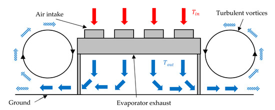
Figure 1.
2D sketch of flow recirculation around a horizontal evaporator, with .
The flow around the evaporator is generally turbulent, due to the large size of the evaporator’s body, with the result of the formation of turbulent vortices on its side, as shown in Figure 1. These vortices will form secondary flow patterns and create recirculation. The recirculation is defined by the amount of cold air, entrained by the vortices, circulating back to the intakes of the evaporator. The recirculation ratio was defined as:
A ratio corresponds to no recirculation and corresponds to a full recirculation.
In addition to the flow velocity and direction, the vortex size, intensity and locations vary with the size and the number of evaporators. The vortices may appear small at the start of the evaporator and increase in size and intensity along the main flow direction. Given the complexity of the flow structure and the number of parameters involved, a CFD approach seems to be a suitable tool to give a good understanding of the recirculation effect.
The air recirculation for ASHPs was investigated using CFD for two different test cases. The first test case represented the horizontal evaporators in a uniform field (flat topology and free of obstacles), whereas the real field topology was added for the second test case.
2.1. Test Case 1: Uniform Field
The CFD model was based on the ASHP located in the Danish city of Brædstrup. The Brædstrup heat pump is composed of 20 horizontal evaporators placed in-line. Each evaporator is composed of eight air intakes and a single outlet. The evaporator model is the AlphaLaval Lu-Ve BD-1000, with its dimensions summarised in Table 1.

Table 1.
Dimensions of the AlphaLaval Lu-Ve BD-1000 evaporator.
The evaporators are joined in groups of two, with a short distance of 0.6 m between two consecutive groups, to allow human maintenance. The evaporators form two symmetry planes, which allows for restricting the simulations to a range of 90°. Therefore, five simulations have been carried out for five wind directions within the 90° angle range: South (S) to east (E) with three intermediate angles separated by 22.5°, as shown in Figure 2.
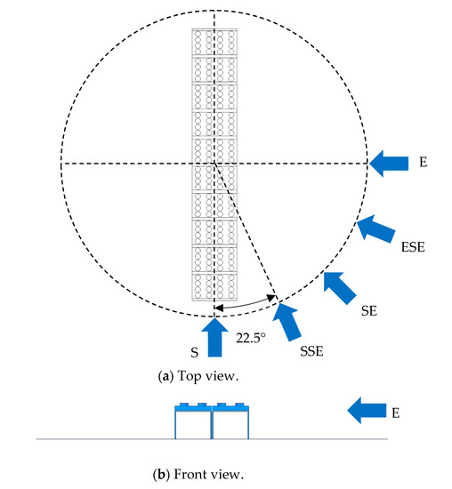
Figure 2.
Sketch of the 20 evaporators, from top view (a) and front view (b), under different wind conditions in the computational fluid dynamics (CFD) simulations, for a uniform field.
The domain size around the evaporators is discussed in Section 2.4.1.
2.2. Test Case 2: Real Field
The Brædstrup real field corresponds to the actual environment where the heat pump is located in the city of Brædstrup. However, the topology was simplified to include only the elements having the most predominant effect on the recirculation. The real field topology includes:
- The 20 evaporators, in the same configuration as for test case 1,
- A building placed at a distance of 16.3 m from the evaporators to the west,
- A ground depression located 1 m from the evaporators to the east. The depression starts gradually to reach a depth of 2 m, at a 3 m distance from the evaporators.
Other elements, such as piping, pumps, electric installations (etc.), were omitted due to their supposed low interference in the flow recirculation. This assumption has the beneficial effect of simplifying the CFD simulation, by keeping a reasonable meshing size. The topology of the real field model is shown in Figure 3, with all dimensions and flow conditions.
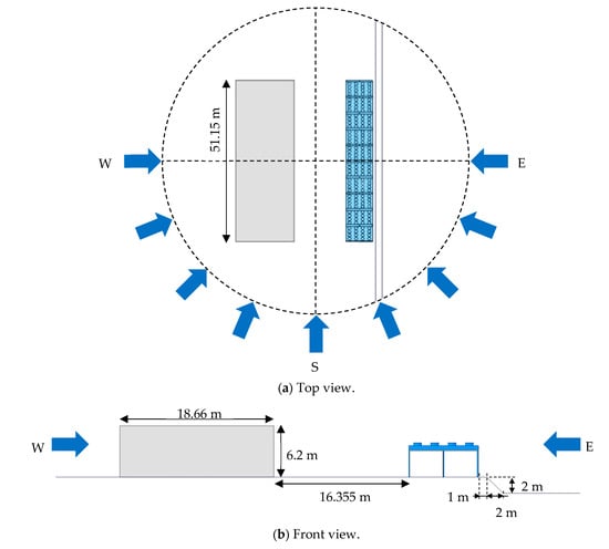
Figure 3.
Sketch of the 20 evaporators from top view (a) and front view (b), with building and ground depression, under different wind conditions in the CFD simulations.
The presence of the building and the ground depression reduces the symmetry to only the W-E plane. Therefore, the number of simulations was increased to nine, while the north wind cases were extrapolated from the results of the south wind condition.
2.3. Modelling Assumptions
Several modelling assumptions were applied to model the flow around the evaporators. First, inner geometries of the evaporator, such as the fins and tubes of the heat exchanger and the fans, were disregarded. Modelling the whole geometry would require a prohibitive amount of mesh nodes to cover the broad range of scale, from the order of millimetres (fins) to decametres (buildings). The evaporator was therefore modelled as a “black box” with inlets, corresponding to the intake of the air entrained by the fans, and an outlet, corresponding to the exhaust of the heat exchanger. The assumptions used in the CFD model were:
- The swirl generated by the fans was not accounted for. However, it was assumed that the flow entering the heat exchanger would become mostly unidirectional due to the restriction of the free flow area in the fins and tubes region.
- No pressure drop was modelled along the fans and the heat exchanger. It is believed that it has a low effect on the recirculation ratio, as is shown in [7,8] or [10]. Pressure variation would be only a result of the flow motion around the evaporator.
- The heat exchanger was modelled implying a temperature drop of 4 K between the ambient air temperature and the evaporator outlet temperature. The heat exchanger performance was not considered in this study, only the recirculation ratio.
- The fluid was assumed incompressible since the diffusive heat transfer was assumed to be predominant compared to the natural convection, due to the high wind velocity.
2.4. 3D Model and Calculation Domain
The 3D model of the evaporator was placed in a larger domain to model the surrounding flow. Considering the large size of the evaporators, especially in the case of multiple devices placed side by side, such as for the given case study, the general guidelines of Franke et al. [15] for CFD simulation of flows in the urban environment were applied. The CFD simulations were performed using the commercial solver Fluent v19.2 from ANSYS.
2.4.1. Domain Size
The domain around the evaporator was expanded in all directions to properly model the flow around the obstacle. Considering a building height , the blockage ratio in the flow direction should be less than 3%, based on the experience of wind tunnel experiments and CFD simulations, as described by Franke et al. [15] and Yoshihide et al. [16]. The blockage ratio corresponds to the ratio of the projected area of the obstacle in the flow direction to the cross-section area of the domain in the flow direction. The vertical extension should be at least to avoid any artificial acceleration of the flow since upper boundary conditions generally do not allow the flow to leave the domain (similar to wind tunnel experiments). In lateral directions, the factor for the extended length was chosen to reflect the minimum blockage ratio of 3%. In the flow direction, upstream, the distance could be reduced to if the ground topology is flat. The inlet boundary condition was modified to include the effect of the wind boundary layer. Finally, the extension in the flow direction, downstream, was the largest with to allow re-development of the flow in the wake region. The boundary condition at the outlet was chosen to allow flow to enter back into the domain in case of a large wake region.
2.4.2. Governing Equations
The CFD model is based on the resolution of the Navier–Stokes equations, which are discretised and solved numerically using the finite volume method (FVM). The mass, velocity and energy balance are done at all cells of the global mesh, which are defined by the continuity equations. The continuity equations are expressed using the Reynolds-averaged Navier–Stokes (RANS) for turbulent flows, with density-weighted time-averaged term written using the common norm .
where is the density, is the flow velocity, is the pressure, is the viscous stress tensor, are the Reynolds stresses, is the gravity, is the total energy, is the heat flux and is the internal heat generation. Equation (2) corresponds to the continuity equation, Equation (3) the momentum equation and Equation (4) the energy equation. The viscosity term is described by Equation (5).
where is the molecular viscosity. The Reynolds stresses are expressed as a function to the mean velocity gradients by employing the Boussinesq hypothesis, used for the Spallart–Allmaras turbulence model, the k-ε models and the k-ω models.
where is the turbulent viscosity and the kinetic energy. The turbulent viscosity is solved by introducing two additional transport equations: One for the kinetic energy and another one for the turbulence equation rate ε (for the k-ε turbulence model). These two governing equations are described by the two following equations.
where and represent the generation of turbulent kinetic energy due to the mean velocity gradient and buoyancy, respectively, , and are constants, and are the turbulent Prandtl numbers for and , respectively, and are source terms. Finally, the turbulent viscosity is computed using the following equation.
2.4.3. Boundary Conditions
The inlet boundary condition was a velocity inlet, with a specified wind profile to account for the effect of the wind boundary layer, thus allowing us to considerably reduce the domain size upstream of the evaporator and ensure a physical representation of the wind profile. The profile was determined by a preliminary 2D CFD simulation, where the inlet and outlet were periodic. The mass flow rate between the inlet and the outlet was calculated to give a desired average velocity. The inlet wind was therefore assumed to be two-dimensional (no variation in the lateral direction) with the assumption of no swirls present upstream of the evaporators. The velocity profile is shown in Figure 4 for an average velocity of 3.7 m/s.
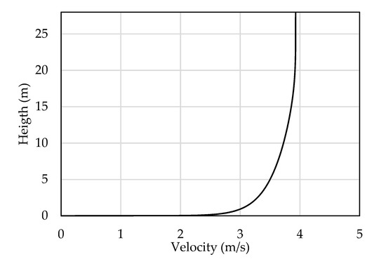
Figure 4.
Inlet velocity profile in the function of the height of the domain.
The outlet boundary condition was a constant static pressure boundary condition where recirculation of the flow back into the domain was allowed, to account for the formation of vortices far away from the obstacle. Symmetries were used for the lateral and upper boundary conditions, which forced the flow to have zero normal velocity at the planes and zero normal gradients of all variables. This is true only at a location far away from the evaporators, if the main flow is not impacted by the obstacle. The ground and the evaporator walls were considered as no-slip adiabatic walls ().
Finally, the air intake was modelled as a mass flow outlet (the flow leaves the domain) and the outlet of the evaporator as a mass flow inlet (the flow enters the domain) at a constant temperature . The difference in the mass flow rates was set zero to ensure mass balance.
2.4.4. Meshing and Turbulence Models
The mesh was built to capture the complexity of vortex formation and dissipation on the sides and in the wake of the evaporators. An inflation layer was applied on the ground surface with a , corresponding to the use of the realisable k-ε turbulence model. The choice of the realisable k-ε turbulence model was motivated by the studies [22,23,24,25], where it is concluded that the modified k-ε turbulence models generally capture the flow behaviour around squared obstacles accurately, although with noticeable overestimation concerning the size of the wake area. An inflation layer could not be generated close to the evaporator walls due to their complex geometry. Instead, the mesh was locally refined close to the evaporator walls, and slowly increased in size along all directions. The use of a wall function ensured that the boundary layer region was correctly modelled for local values of . The mesh was also fully structured to avoid numerical diffusion. Figure 5 shows the evolution of the average inlet temperature at the intakes of the evaporators, as a function of the mesh size. The mesh independence study shown in Figure 5 was carried out for a wind coming from the south direction.
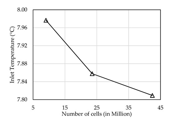
Figure 5.
Evolution of inlet temperature as a function of mesh size.
The difference in temperature between the second and third mesh (23.5 and 42.4 M cells, respectively) was lower than 1%. Therefore, to keep a reasonable mesh size and calculation time, the second mesh was kept for further investigations. Figure 6 shows the mesh at the evaporator walls and ground.
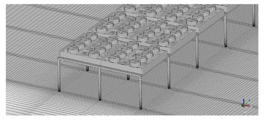
Figure 6.
Mesh of the 20 evaporators (first 12 rows), at the wall surfaces.
The cell density is increased at the foot of the evaporators’ legs due to the wind boundary layer. The cells’ size increases as the distance from the walls increases. However, conformal meshing is used to keep a cell number ratio of 1 to 1 between two adjacent cells, to increase the mesh accuracy and quality. The mesh quality, in term of orthogonality, is very high with an average value of 0.996 (1 being the maximum) and a minimum value of 0.649. The average value for the skewness is equal to 0.0235 (0 for equilateral) and with a maximum value of 0.641. The effect of having a high-quality mesh is a faster and smoother convergence, as well as minimisation of the numerical errors due to distorted cells. The increase in the mesh size for keeping a constant cell-to-cell ratio and a high mesh quality is compensated by the use of HPC to perform the simulations.
3. Results for a Uniform Field
The domain size for the uniform field was updated as a function of the wind direction, to account for the change of the flow frontal area of the evaporators. The mesh size of all configurations ranged from 24 to 26 M nodes. The simulations were carried out using 32 cores of an Intel Xeon CPU E5-2670 @ 2.6 GHz and 64 GB of RAM. The simulation time was approximately 2 days for 20,000 iterations.
The inputs of the CFD simulations for the evaporators placed in a uniform field are summarised in Table 2.
Table 2.
Boundary conditions of the CFD model.
The inlet average velocity and temperature correspond to the average velocity and temperature for the last 10 years at the city of Horsens, the closest city with available data from Danmarks Meteorologiske Institut (DMI). These average values also correspond to the most prevalent wind and temperature conditions on any given day in the area (except during the peak of winter and summer).
3.1. South Wind Condition
First, the simulation for a south wind direction was carried out. Velocity vectors at different cross-sections are shown in Figure 7, where the large blue arrow indicates the wind direction.
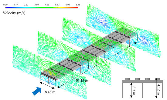
Figure 7.
Velocity vectors at different locations of the evaporators, uniform field and south wind condition.
As expected, the flow becomes turbulent on the sides of the evaporators with the formation of vortices. These vortices grow in size as the air flows downstream, as pointed out by Owen and Kröger [14], and move away from the lateral sides of the evaporator. These vortices are created by the combination of (1) the blockage of the main flow by the evaporators, which induces energy dissipation by vortex formation and (2) the exhaust flow leaving the evaporator exhaust towards the ground and mixing with the surrounding air. The associated temperature contours at the same locations are shown in Figure 8.
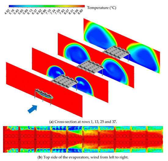
Figure 8.
Temperature contour at different locations of the evaporators (a) and temperature contour on the top side of the evaporators (b) uniform field and south wind condition.
The recirculation appears at the second row of the fan intakes and only affects the lateral fans. The intensity increases along the flow direction according to the development of the vortices. However, the recirculation starts to decrease at the 18th row (9th evaporator), with a rapid increase in the temperature at the inlets, as can be seen in Figure 8b. The recirculation remains rather constant from the 24th row until the last row. The sudden decrease in recirculation ratio is due to the displacement of the lateral vortices away from the evaporators. This phenomenon can be explained by a gradual loss in kinetic energy of the main wind flow below the evaporators, due to the exhaust flow partially blocking the wind. Therefore, at a certain distance, the exhaust air starts to flow in all directions, pushing the vortices further away from the evaporators. Figure 9 shows that the change of direction of the exhaust air starts at the 9th evaporator, corresponding to the local change of recirculation ratio. Overall, the average recirculation ratio for the south wind condition is = 26.4%.
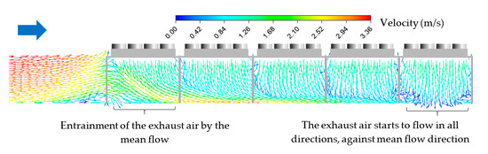
Figure 9.
Velocity streamlines below the evaporators, uniform field and south wind condition.
The displacement of the vortex centres away from the lateral sides of the evaporator can also be seen in Figure 10. Figure 10 presents the vortex region of the domain, using the method. The method was defined by Jeong and Hussain [26], and represents the excess of rotation rate over the strain rate magnitude on a specific plane. Therefore, the values of can be shown by iso-surfaces for negative values of , which indicate the presence of vortices.
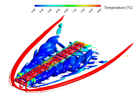
Figure 10.
Vortex region of the flow around the evaporators with associated temperature field, uniform field and south wind condition.
The horseshoe vortex (in red) is a typical vortex type encountered for flow around an obstacle [27]. It represents the boundary region where the wind starts to be impacted by the presence of the obstacle. The horseshoe vortex is red (ambient temperature), which indicates that there is no mixing of the ambient air and the colder flow leaving the exhaust of the evaporators outside of this region. On the other hand, the main vortices responsible for recirculation are shown in blue alongside the evaporators. It clearly shows that the cold air is entrained by the lateral vortices and recirculates back to the evaporator intakes. The smaller red vortices on top of the evaporators are due to the presence of the rounded fan intakes, which disturb the flow at a lower magnitude.
3.2. East Wind
The domain size was updated and the same boundary conditions as the south wind case were applied. Figure 11 shows the velocity vector and temperature contour at the 21st row and at the top side of the evaporators.
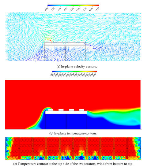
Figure 11.
Velocity vectors (a) and temperature contour (b) at the cross-section of row 21 and temperature contour at the top side of the evaporators (c), uniform field and east wind condition.
The kinetic energy of the wind is not sufficient to entrain the exhaust flow downstream, which creates recirculation at the first row of the fan intakes in addition to the lateral intakes. However, the recirculation drops at the second row, and becomes negligible for the 3rd and 4th row, except on the lateral sides where recirculation increases. Overall, the average recirculation is equal to = 16.9%, which is lower than for the south wind condition, since fewer fan intakes are impacted by the recirculation.
3.3. South-East Wind
In these cases, the wind attacks two sides of the evaporators. The velocity components were adjusted depending on the angle formed by the wind direction with the reference vector (south) by using basic trigonometric laws. The temperature contour of the evaporators (top view) is shown in Figure 12 for all wind directions.
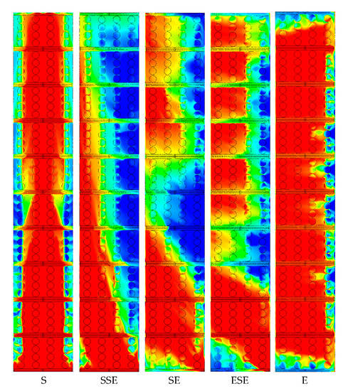
Figure 12.
Temperature contour of the evaporators (top side), uniform field and all directions.
The corresponding global recirculation ratio for all wind directions is shown in Figure 13. The results have been extrapolated for 360° due to the two symmetry plans of the geometry.
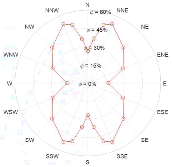
Figure 13.
Global recirculation at the intakes of the evaporators, uniform field.
Two additional simulations were added to refine the results close to the maximum recirculation. Figure 13 shows that the recirculation is the lowest ( = 16.9%) for west and east directions, and the highest ( = 52.5%) for SSW, SSE, NNW and NNE, which corresponds to an angle of +/−22.5° from the north or south direction. This high recirculation ratio can be explained by the combination of several factors:
(1) If the wind direction is not parallel to one of the main directions of the evaporators (N, E, S or W), there is the combined effect of having recirculation on the lateral intakes due to the formation of turbulent vortices, as well as recirculation on the front row due to the relatively low kinetic energy of the wind.
(2) In addition to the turbulent mixing, the wind pushes the vortices towards the upper side of evaporators, due to higher velocity at a higher altitude, which increases the amount of cold air recirculating back to the evaporators’ inlets.
Figure 14 represents the temperature contour at different cross-sections of the evaporators, for SSE (worst case condition) and south wind conditions. It clearly shows that the lateral component of the wind in the SSE case carries the vortices towards the upper side of the evaporators, which propagates the recirculation to the inner fan intakes. Concerning the southern wind, the recirculation is limited to the lateral intakes.
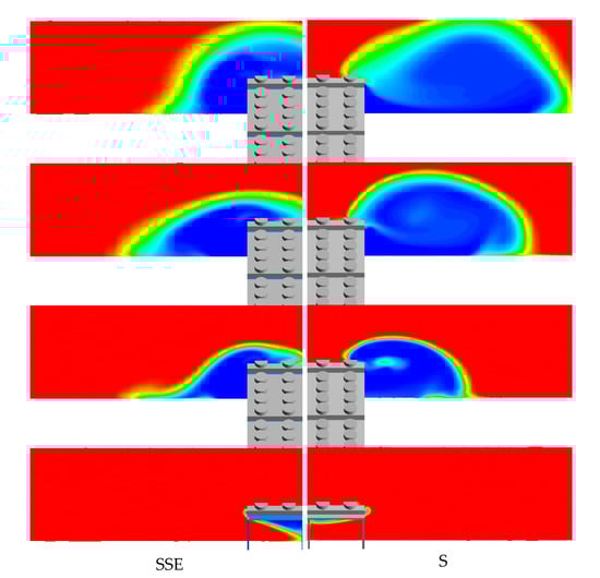
Figure 14.
Temperature contour at different cross-sections (rows 1, 13, 25 and 37) for SSE (left) and S (right) wind directions, uniform field.
4. Results for Real Field Topology
The boundary conditions remained the same as for the uniform field simulations, except for the velocity inlet of the domain. Unlike the uniform field case, the inlet velocity profile was not only dependent on the altitude, but also on the lateral position due to a non-uniform ground level. Consequently, the inlet velocity profile was preliminarily computed by simulating a thin portion of the domain, without any obstacles. The model is shown in Figure 15.
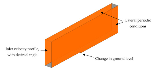
Figure 15.
Preliminary CFD model for determining the inlet velocity profile of the real topology model.
The inlet velocity profile included the wind boundary layer (seen in Figure 4), as well as the wind direction. The lateral periodic conditions force the flow to behave similarly at these two locations. By doing so, the flow inside the domain was forced to follow the angle given at the inlet, while taking into account the effect of the ground depression along the flow direction. The upper surface remains a symmetry plane and the surface opposite to the inlet was set to a pressure outlet. The velocity profile on one of the periodic sides was exported from the preliminary simulation and imported into the final CFD simulation as a velocity inlet.
Finally, the mesh size of the whole model, for all wind configurations, ranged from 35 to 45 M nodes. The simulations were carried out using 96 cores of an Intel Xeon CPU E5-2670 @ 2.6 GHz and 64 GB of RAM. The simulation time was approximately 3 days for 20,000 iterations.
4.1. South Wind
Figure 16 shows the temperature contour around the building and the evaporators at different cross-sections. Similar to the uniform field in Section 4, the vortices grow in size and move away from the evaporators along the flow direction. Lower intensity vortices appear along the building, as well as in the ground depression, due to the sudden change of direction. The locations of the recirculation vortex centres are similar when compared with the uniform field but have different sizes and shapes, which indicates that the presence of a building or a ground depression has a non-negligible influence on the recirculation rate.
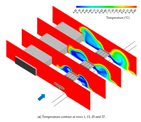
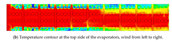
Figure 16.
Temperature contour (a) at different cross-sections and temperature contour at the top side of the evaporators (b), real field and south wind condition.
As can be seen in Figure 16b, the temperature contour is not symmetrical on the two lateral sides of the evaporators. On the building side, the recirculation to the lateral inlets decreases along the flow direction, due to the separation of the vortices from the evaporator side. However, cold air starts to reach the 2nd line of intakes from the 25th row, which corresponds to the position where the vortices reach the building. The building creates a channel on the west side of the evaporator, which forces the vortices to expand in the limited space between these two obstacles and reach the inner evaporator inlets.
On the other hand, the recirculation is lower on the ground depression side. The sudden change of the ground direction creates additional recirculation zones, which locally increases the energy dissipation. Figure 17 shows the turbulent eddy dissipation rate at row 17. The turbulent eddy dissipation rate is higher on the ground depression side compared with the building side, which indicates that there is an enhanced mixing between the cold exhaust stream and the ambient air, resulting in a lower recirculation rate. The total flow recirculation is equal to = 21.9%, which is 17% lower compared to the uniform case with = 26.4%.
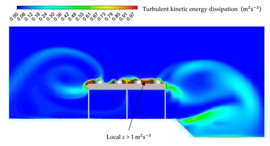
Figure 17.
Turbulent kinetic energy dissipation contour at the cross-section of row 17, real field and south wind condition.
4.2. West Wind
The west wind condition has the particularity of having the evaporators in the wake of the building, which results in a distorted wind profile upstream of the evaporators. Figure 18 shows the velocity vectors and temperature contour at row 17 for west wind conditions.
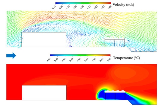
Figure 18.
Velocity streamlines and temperature contour at row 17, real field and west wind condition.
As expected, recirculation zones appear in the wake of the building, which leads to a lower flow velocity upstream of the evaporators and eventually to a change in main flow direction depending on the vortex sizes and intensities. The recirculation intensity depends on the location in the wake of the building. The strongest vortices appear at the centre of the wake region, with a decreasing intensity while moving towards the lateral sides of the building. This effect is shown in Figure 19, which represents the temperature contour on the top of the evaporators.
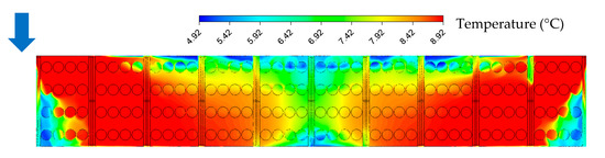
Figure 19.
Temperature contour of the evaporators (top side), no building (up), real field (down) and west wind condition.
Overall, due to the presence of a large obstacle upstream of the evaporators, the total flow recirculation reaches = 20.9%, which is 23.8% higher compared to the perfect field with = 16.9%.
4.3. East Wind
For east wind, the recirculation is largely influenced by the ground depression. Figure 20 shows the velocity vectors and temperature contour at row 17.
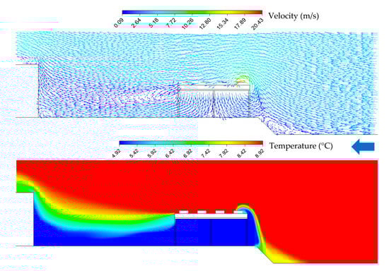
Figure 20.
Velocity streamlines and temperature contour at row 17, real field and east wind condition.
Similar to the west wind condition, the ground depression induces dissipation of kinetic energy due to the sudden change in ground level and results in additional recirculation zones. This results in an overall recirculation ratio of 13.1%, which is 22.7% lower compared to the uniform field with φ = 16.9%. It may be noticed that the building does not have any influence on the recirculation due to the large distance between the two obstacles.
4.4. All Wind Conditions
Figure 21 represents the recirculation rate in function of the angle of the wind, for both uniform field and real field conditions.
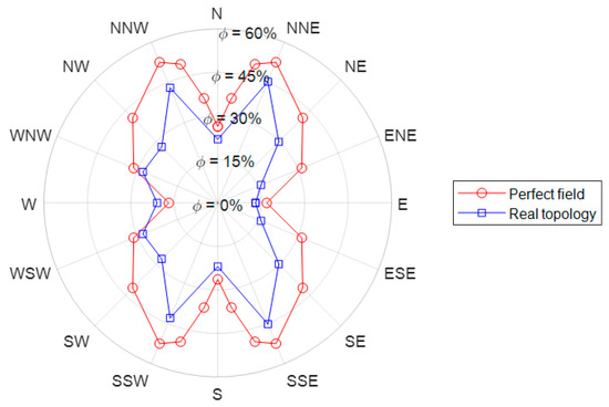
Figure 21.
Global recirculation at the intakes of the evaporators, uniform field (red) and real topology (blue).
First of all, there is a global decrease in recirculation of 28% for the real topology, compared with the uniform field case. The recirculation ratio is higher for the real topology only for the west wind condition, where the evaporators are aligned in the wake of the building. However, the opposite is the case for all other wind directions, which result in a decreased recirculation ratio due to a global reduction in wind velocity upstream of the evaporators.
The east wind cases show a rather constant decrease in recirculation ratio, whichever the wind direction, due to the ground depression and local loss of turbulent kinetic energy of the exhaust flow of the evaporator.
Overall, the lowest recirculation appears for the east wind condition with = 13.1% with a low variation if the wind deviates slightly from the eastern direction. It is therefore recommended to place the evaporators in the crosswind direction where the number of lateral inlets, which might be impacted by the lateral vortices, is the lowest. Furthermore, the average recirculation rate (for real topology) is equal to 27.6%, which will lead to a significant decrease in the COP of the heat pump by lower inlet temperatures.
5. Discussion
The results obtained from CFD simulations describe the complete flow field around the evaporators in term of velocity, temperature and pressure. Obtaining the same detailed results from an experimental investigation would be very difficult considering the geometry of the evaporators and the required number of sensors to capture the flow field along the 51 m of evaporators. A CFD model, therefore, seems to be a suitable tool to provide an initial investigation of the influence of the wind, ground topology and surrounding obstacles on the cold air recirculation of ASHPs.
On the other hand, the numerical results are based on several assumptions and simplifications, which always should be kept in mind. The complexity of the inner and outer geometry of the evaporators had to be reduced to model the air recirculation. As mentioned in Section 3, the main assumption of the CFD model was to completely disregard the inner geometry of the evaporators including the fans and the fins and tubes of the heat exchanger. Consequently, the modelling of the heat transfer inside the evaporators was simplified to a fixed temperature drop of 4 K between the ambient air temperature and the temperature at the evaporator outlet. Therefore, several physical phenomena were omitted in the CFD simulations, such as:
- The effect of swirl and non-uniform flow generated by the fan: In between the fan and the fin and tube heat exchanger, the flow will be strongly impacted by the swirl generated by the fan. However, inside the fin and tube heat exchanger, the free flow area is reduced and the motion of the air flow will become mostly unidirectional along the heat exchanger, guided by the evaporator fins. The assumption of unidirectional flow at the exhaust of the evaporators therefore seems reasonable. However, the flow velocities might in reality not be uniform, with higher velocities below the fans and lower air velocities in the areas between fans. A non-uniform airflow at the outlet was not considered in the present CFD analysis and could affect the validity of the results.
- The pressure change in the fans and the heat exchanger: In the case of flow entering the heat exchanger downstream of a fan, the fan has to provide an increase in static pressure corresponding to, at least, the pressure drop inside the heat exchanger. In the present CFD model, a balance in the pressure variation inside the evaporator was assumed, where the static pressure at the inlet and outlet were considered equal. It is assumed that the effects of this assumption of the validity of the results are small.
- The heat transfer in the heat exchanger: The heat transfer rate inside the heat exchanger would be a function of the flow speed and temperature at the inlet of the evaporator. For the real evaporators, the temperature at the evaporator exhaust will vary depending on the recirculation ratio and chaotic flow behaviour around the evaporators. This was not included in the present CFD model.
Other parameters such as the humidity level, the presence of liquid droplets (for rainy conditions) or the solar radiation were not integrated into the CFD simulations.
The impact of these modelling assumptions on the validity of the results should be investigated by an experimental validation of the results in the future once the given ASHP is in operation. However, the complexity of a CFD model is typically linked to the available resources and the scale of the studied geometry. For the given case, the assumptions are believed to provide a reasonable balance between complexity and validity to investigate the cold air recirculation alone.
As mentioned in the introduction, the choice of a turbulence model has a major impact on the estimation of the turbulence scale of the flow around the evaporators. The RANS turbulence models, such as the realisable k-ε model applied in the present study, generally overestimate the wake region behind buildings, as summarised by Shirzadi et al. [28]. The prediction of the RANS simulation can be improved by changing the semi-empirical coefficients of the turbulence models. However, these coefficients are strongly related to the flow problem and are generally derived from experimental results, which are lacking in the present study. The use of more advanced turbulence models, such as LES or DNS, show more accurate results in capturing the wake region and the vortex intensity around buildings, as reported by Liu and Niu [29]. Nevertheless, the gain in accuracy is counterbalanced by the significant increase in computing power required to run the unstable CFD simulations. Considering the complexity of the evaporator geometry and mesh size (>40 M cells), the RANS turbulence models were preferred for this study.
Finally, the results of this study show that recirculation occurs for all wind directions due to the inherent turbulent behaviour of the flow around the evaporators. This is a crucial outcome to point out for ASHP designers since the inlet temperature of the evaporator will most likely be lower than the expected ambient air temperature. Furthermore, the recirculation is greatly influenced by the wind direction, the geometry of the evaporators and the field topology, which makes difficult to give a right estimation of the recirculation rate. As a general output, it is relevant to assume a decrease in the evaporator’s inlet temperature of ~20%, as a “worst-case condition”, to involve the effect of the cold air recirculation in an ASHP model.
6. Conclusions
The rapid expansion of large-scale air-source heat pumps in urban environments requires that more effort should be dedicated to understand the effect of their surroundings on their performances. This paper provides a first estimation of the cold air recirculation for the evaporators of an ASHP, using a CFD model. The air recirculation was studied for two different ASHP field topologies, with the aim to give useful insights about the effect of close obstacles on the air recirculation around the ASHP’s evaporators.
The results show that cold air recirculation occurs whichever the wind direction, with a global recirculation ratio of 38.3% and 27.6% for the uniform field and the real field, respectively. The recirculation was generated by the formation of vortices on the sides of the evaporators, which catch and recirculate the cold exhaust air of the evaporators back to the fans’ inlets. It appeared that the presence of a building upstream of the evaporators intensified the recirculation due to the presence of turbulent vortices in its wake. On the other hand, a small ground depression (2 m) close to the evaporators helped to reduce the recirculation by dissipating part of the energy of the cold exhaust air of the evaporators, due to the sudden change in ground direction.
Overall, the cold air recirculation was not negligible, with a minimum ratio of 13.1% (pure crosswind wind) and a maximum ratio of 45.2% for the worst-case condition (transverse wind), for the real field topology. These results highlight the need to consider the decrease in the average evaporator inlet temperature when estimating the coefficient of performance (COP) of an air-source heat pump since it will most likely never work without cold air entrainment.
Finally, this study gives an initial understanding of the flow condition to optimise the placement of the evaporators depending on the wind condition, but also explores possible designs to reduce the air recirculation.
Author Contributions
Conceptualization, B.R., J.K.J., S.O.K.H. and W.B.M.; methodology, B.R., J.K.J., S.O.K.H. and W.B.M.; software, B.R.; validation, B.R.; formal analysis, B.R. and W.B.M.; investigation, B.R.; resources, B.R.; data curation, B.R.; writing—original draft preparation, B.R., J.K.J. and W.B.M.; writing—review and editing, B.R. and W.B.M.; visualization, B.R.; supervision, S.O.K.H. and W.B.M.; project administration, S.O.K.H. and W.B.M.; funding acquisition, S.O.K.H. and W.B.M. All authors have read and agreed to the published version of the manuscript.
Funding
This research was funded by the Energy Technology Development and Demonstration Program (EUDP), grant number EUDP2019-I “AirToHeat”.
Conflicts of Interest
The authors declare no conflict of interest.
References
- David, A.; Mathiesen, B.V.; Averfalk, H.; Werner, S.; Lund, H. Heat Roadmap Europe: Large-scale electric heat pumps in district heating systems. Energies 2017, 10, 578. [Google Scholar] [CrossRef]
- Available online: https://www.danskfjernvarme.dk/presse/fakta-om-fjernvarme (accessed on 1 September 2020).
- Lund, R.; Ilic, D.D.; Trygg, L. Socioeconomic potential for introducing large-scale heat pumps in district heating in Denmark. J. Clean. Prod. 2016, 139, 219–229. [Google Scholar] [CrossRef]
- Bach, B.; Werling, J.; Ommen, T.; Münster, M.; Morales, J.M.; Elmegaard, B. Integration of large-scale heat pumps in the district heating systems of Greater Copenhagen. Energy 2016, 107, 321–334. [Google Scholar] [CrossRef]
- Kröger, D.G. Reduction in performance due to recirculation in mechanical draft cooling towers. Heat Transf. Eng. 1989, 10, 37–43. [Google Scholar] [CrossRef]
- Duvenhage, K.; Kröger, D.G. The influence of wind on the performance of forced draught air-cooled heat exchangers. J. Wind Eng. Ind. Aerodyn. 1996, 62, 259–277. [Google Scholar] [CrossRef]
- Rogers, J.A.; Won, K.; Stang, W. Validation of CFD Models for Evaluating Hot-Air Recirculation in Air-Cooled Heat Exchangers. In Proceedings of the AIChE Spring Meeting, Houston, TX, USA, 14–18 March 1999. [Google Scholar]
- Borghei, L.; Ramin, K. Wind effects on air-cooled condenser performance.‖ New Aspects of Fluid Mechanics. In Proceedings of the Heat Transfer, and Environment, 8th IASME/WSEAS International Conference on Fluid Mechanics and Aerodynamics, Taipei, Taiwan, 20–22 August 2010. [Google Scholar]
- Maulbetsch, J.S.; DiFilippo, M.N.; O’Hagan, J. Effect of wind on Air-Cooled condenser performance. In Proceedings of the ASME 2011 International Mechanical Engineering Congress and Exposition, Denver, CO, USA, 11–17 November 2011; Volume 1, pp. 391–396. [Google Scholar] [CrossRef]
- Liu, P.; Duan, H.; Zhao, W. Numerical investigation of hot air recirculation of air-cooled condensers at a large power plant. Appl. Therm. Eng. 2009, 29, 1927–1934. [Google Scholar] [CrossRef]
- Kong, Y.; Wang, W.; Huang, X.; Yang, L.; Du, X.; Yang, Y. Circularly arranged air-cooled condensers to restrain adverse wind effects. Appl. Therm. Eng. 2017, 124, 202–223. [Google Scholar] [CrossRef]
- Jin, R.; Yang, X.; Yang, L.; Du, X.; Yang, Y. Square array of air-cooled condensers to improve thermo-flow performances under windy conditions. Int. J. Heat Mass Transf. 2018, 127, 717–729. [Google Scholar] [CrossRef]
- Yang, L.J.; Du, X.Z.; Yang, Y.P. Influences of wind-break wall configurations upon flow and heat transfer characteristics of air-cooled condensers in a power plant. Int. J. Therm. Sci. 2011, 50, 2050–2061. [Google Scholar] [CrossRef]
- Owen, M.; Kröger, D.G. Contributors to increased fan inlet temperature at an air-cooled steam condenser. Appl. Therm. Eng. 2013, 50, 1149–1156. [Google Scholar] [CrossRef]
- Franke, J.; Hellsten, A.; Schlünzen, H.; Carissimo, B. Best Practice Guideline for the CFD Simulation of Flows in the Urban Environment; University of Hamburg: Hamburg, Germany, 2007; ISBN 3-00-018312-4. [Google Scholar]
- Tominaga, Y.; Mochida, A.; Yoshie, R.; Kataoka, H.; Nozu, T.; Yoshikawa, M.; Shirasawa, T. AIJ guidelines for practical applications of CFD to pedestrian wind environment around buildings. J. Wind Eng. Ind. Aerodyn. 2008, 96, 1749–1761. [Google Scholar] [CrossRef]
- Spalart, P.R.; Allmaras, S.R. A One-equation turbulence model for aerodynamic flows. AIAA J. 1992, 5–21. [Google Scholar] [CrossRef]
- Jones, W.P.; Launder, B.E. The prediction of laminarization with a two-equation model of turbulence. Int. J. Heat Mass Transf. 1972, 15, 301–314. [Google Scholar] [CrossRef]
- Shih, T.-H.; Liou, W.W.; Shabbir, A.; Yang, Z.; Zhu, J. A new k-e Eddy Viscosity Model for High Reynolds Number Turbulent Flows. Comput. Fluids 1995, 24, 227–238. [Google Scholar] [CrossRef]
- Yakhot, V.; Orszag, S.A. Renormalization group analysis of turbulence. I. Basic theory. J. Sci. Comput. 1986, 1, 3–51. [Google Scholar] [CrossRef]
- Menter, F.R. Two-equation eddy-viscosity turbulence models for engineering applications. AIAA J. 1994, 32, 1598–1605. [Google Scholar] [CrossRef]
- Yoshie, R.; Mochida, A.; Tominaga, Y.; Kataoka, H.; Harimoto, K.; Nozu, T.; Shirasawa, T. Cooperative project for CFD predictionof pedestrian wind environment in the Architectural Institute of Japan. J. Wind Eng. Ind. Aerodyn. 2007, 95, 1551–1578. [Google Scholar] [CrossRef]
- Li, B.; Liu, J.; Luo, F.; Man, X. Evaluation of CFD Simulation Using Various Turbulence Models for Wind Pressure on Buildings Based on Wind Tunnel Experiments. Procedia Eng. 2015, 121, 2209–2216. [Google Scholar] [CrossRef]
- Tominaga, Y.; Akabayashi, S.I.; Kitahara, T.; Arinami, Y. Air flow around isolated gable-roof buildings with different roof pitches: Wind tunnel experiments and CFD simulations. Build. Environ. 2015, 84, 204–213. [Google Scholar] [CrossRef]
- Ntinas, G.K.; Shen, X.; Wang, Y.; Zhang, G. Evaluation of CFD turbulence models for simulating external airflow around varied building roof with wind tunnel experiment. Build. Simul. 2018, 11, 115–123. [Google Scholar] [CrossRef]
- JEong, J.; Hussain, F. On the identification of a vortex. J. Fluid Mech. 1995, 285, 69–94. [Google Scholar] [CrossRef]
- Hosker, R.P. Flow and diffusion near obstacles. In Atmospheric Science and Power Production, Technical Information Center; Randerson, D., Ed.; U.S. Department of Energy: Washington, DC, USA, 1984; pp. 241–326. [Google Scholar]
- Shirzadi, M.; Mirzaei, P.A.; Naghashzadegan, M. Improvement of k-epsilon turbulence model for CFD simulation of atmospheric boundary layer around a high-rise building using stochastic optimization and Monte Carlo Sampling technique. J. Wind Eng. Ind. Aerodyn. 2017, 171, 366–379. [Google Scholar] [CrossRef]
- Liu, J.; Niu, J. CFD simulation of the wind environment around an isolated high-rise building: An evaluation of SRANS, LES and DES models. Build. Environ. 2016, 96, 91–106. [Google Scholar] [CrossRef]
Publisher’s Note: MDPI stays neutral with regard to jurisdictional claims in published maps and institutional affiliations. |
© 2020 by the authors. Licensee MDPI, Basel, Switzerland. This article is an open access article distributed under the terms and conditions of the Creative Commons Attribution (CC BY) license (http://creativecommons.org/licenses/by/4.0/).