Article

Altimetry-Based Diagnosis of Deep-Reaching Sub-Mesoscale Ocean Fronts

by
Lia Siegelman
1,2,*,
Patrice Klein
1,2,3,4,
Andrew F. Thompson
1,
Hector S. Torres
2 and
Dimitris Menemenlis
2
1
Environmental Science and Engineering, California Institute of Technology, Pasadena, CA 91125, USA
2
Jet Propulsion Laboratory, California Institute of Technology, Pasadena, CA 91109, USA
3
Laboratory for Ocean Physics and Satellite remote sensing, Ifremer, CNRS, Univ. de Bretagne Occidentale, 29280 Plouzane, France
4
Laboratoire de Meteorologie Dynamique, Ecole Normale Superieure, CNRS, 75005 Paris, France
*
Author to whom correspondence should be addressed.
Fluids 2020, 5(3), 145; https://doi.org/10.3390/fluids5030145
Submission received: 10 August 2020 / Revised: 23 August 2020 / Accepted: 25 August 2020 / Published: 28 August 2020
(This article belongs to the Special Issue Submesoscale Processes in the Ocean)

Abstract

:
Recent studies demonstrate that energetic sub-mesoscale fronts (10–50 km width) extend in the ocean interior, driving large vertical velocities and associated fluxes. However, diagnosing the dynamics of these deep-reaching fronts from in situ observations remains challenging because of the lack of information on the 3-D structure of the horizontal velocity. Here, a realistic numerical simulation in the Antarctic Circumpolar Current (ACC) is used to study the dynamics of submesocale fronts in relation to velocity gradients, responsible for the formation of these fronts. Results highlight that the stirring properties of the flow at depth, which are related to the velocity gradients, can be inferred from finite-size Lyapunov exponent (FSLE) at the surface. Satellite altimetry observations of FSLE and velocity gradients are then used in combination with recent in situ observations collected by an elephant seal in the ACC to reconstruct frontal dynamics and their associated vertical velocities down to 500 m. The approach proposed here is well suited for the analysis of sub-mesoscale-resolving datasets and the design of future sub-mesoscale field campaigns.

1. Introduction

Recent observational and numerical studies revealed the existence of energetic sub-mesoscale fronts (10–50 km width) in regions of elevated Eddy Kinetic Energy (EKE), not only within the surface mixed layer but also below it down to 900 m [1,2,3,4]. These fronts are characterized by Richardson and Rossby numbers of order one, emphasizing their ageostrophic character [1,3,4]. They result from the horizontal stirring of buoyancy anomalies by mesoscale eddies (50–300 km size) and are associated with intense vertical velocities [5]. Their impact on oceanic vertical heat transport is an order of magnitude larger than the one associated with mesoscale eddies [6]. However, inferring the dynamics of these sub-mesoscale fronts requires knowledge of the evolution of the 3-D structure of the horizontal velocity over a few days, which is rarely accessible from high-resolution in situ data. Only the surface 2-D velocity field at moderate resolution provided by satellite altimeter is commonly available.
This study aims to assess the pertinence of using satellite observations to infer the dynamics of deep-reaching sub-mesoscale fronts. The main goal is to provide a proof of concept of the usefulness of altimetry data to diagnose the dynamics of ocean fronts in existing sub-mesoscale-resolving observations, and to help design future in situ experiments focused on sub-mesoscale dynamics.
To do so, we use outputs from a 1/48 -resolution numerical simulation in the Antarctic Circumpolar Current (ACC) during springtime. The model exhibits deep-reaching buoyancy fronts, from the surface down to 500 m, which are characterized by Rossby and Richardson numbers of order one. Numerical results highlight the vertical homogeneity of the horizontal stirring properties of the flow down to 500 m, suggesting that it is possible to infer subsurface dynamics from surface fields. We then explore the use of Finite-Size Lyapunov Exponent (FSLE), indicative of the stirring properties of the flow integrated over a Lagrangian trajectory, to recover the orientation and growth rate of deep-reaching ocean fronts. Based on the numerical results, we then combine FSLE diagnosed from satellite altimetry with in situ observations collected by a southern elephant seal, in a similar region and season as the model, to recover the correct orientation, magnitude and growth rate of deep-reaching sub-mesoscale fronts and their associated vertical velocities.
The numerical model and observations are presented in Section 2. The proof of concept based on the numerical results is developed in Section 3. Frontal dynamics inferred from the analysis of new seal-sampled observations combined with satellite altimetry data are discussed in Section 4. Finally, a discussion is offered in Section 5.

2. Materials and Methods

2.1. LLC4320 Numerical Simulation

We use the LLC4320 simulation, which is based on a global, full-depth ocean and sea ice configuration of the Massachusetts Institute of Technology general circulation model (MITgcm) [7,8]. It includes tides, has a horizontal resolution of 1 / 48 and 90 vertical levels. We refer the reader to Appendix A of Siegelman [4] and Torres et al. [9] for a full description of the characteristics of this simulation and its validation with observations. A sub-domain of the ACC, east of the Kerguelen Islands and spanning 86–90 E, 48–52 S is analyzed. This domain is one of the highest EKE regions of the ACC and has a thermocline that can be as deep as 600 m, whereas the Mixed Layer Depth (MLD) has a relatively shallow average value of 50 m and local maxima of 100 m within cyclonic eddies. The domain is large enough to capture numerous mesoscale eddies and the resolution is sufficiently high to resolve sub-mesoscale features such as elongated fronts and sub-mesoscale vortices (Figure 1). The time period ranges from 27 October to 27 December 2011, i.e., late spring in the Southern Hemisphere.

Finite-Size Lyapunov Exponent

Finite-Size Lyapunov Exponent (FSLE) is a Lagrangian diagnostic that measures the separation of a pair of initially close particles ( δ X ( t ) , with X ( t ) the position of a particle at time t) embedded in a given flow field. The separation’s growth rate is given by the FSLE’s largest eigenvalue, defined as
λ ( d 0 , d f ) = 1 τ l o g ( d f d 0 ) ,
where d 0 ( d f ) is the initial (final) separation distance and τ the first time at which a separation d f is reached. λ has the dimension of time 1 . FSLE’s eigenvector associated with λ gives the orientation of the particles’ separation. Large λ indicate regions of strong stretching [10]. Noteote that FSLE also characterize the growth rate and orientation of lateral gradients of buoyancy [11,12,13] (see Appendix A for an explanation).
FSLE are computed hourly from the model full velocity field and from the model velocity field after application of a low-pass filter with a cutoff wavelength of 20 km (Appendix C). We choose d 0 = 0.01 and d f = 0.2 to capture mesoscale and sub-mesoscale features [10]. FSLE are computed backward in time (negative values) using the code provided by AVISO and available at https://bitbucket.org/cnes_aviso/lagrangian/src/master/.

2.2. Altimetry Data

We use the Ssalto/Duacs 1/4 delayed-time L4 gridded Sea Surface Height and derived variables provided by Copernicus Marine and Environment Monitoring Service from 6 November to 15 November 2018. The data is available at http://marine.copernicus.eu/services-portfolio/access-to-products/. Vorticity, strain rate and the Okubo-Weiss quantity are computed each day from the altimetry-derived geostrophic velocities.
We use the 1/25 delayed-time FSLE value-added product provided by AVISO from 6 November to 15 November 2018. FSLE are computed backward with d 0 = 0.02 and d f = 0.6 . The data is available at https://www.aviso.altimetry.fr/es/data/products/value-added-products/fsle-finite-size-lyapunov-exponents.html.
Lagrangian time series of geostrophic velocities and FSLE’s orientation are extracted along the seal’s path.

2.3. Southern Elephant Seal Dataset

We analyze a new in situ dataset collected by a female southern elephant seal from October 2018 to January 2019 east of the Kerguelen Islands in the ACC. We refer the reader to the Methods in Siegelman et al. [3] for more details on the data and correction procedure. However, briefly, the seal was equipped with a CTD-SRDL (CTD-Satellite Relay Data Logger) tag recording conductivity, temperature and pressure at a frequency of 0.5 Hz, subsequently interpolated onto a vertical grid of 1 m resolution. The transect of interest spans 500 km between 6 November and 15 November 2018 with a median spacing between two dives of 800 m, and is further discussed in Section 4. In this transect, the maximal depth of a dive is 800 m and more than 90% of the dives are deeper than 200 m, 50% deeper than 400 m and 35% reach 500 m or more. The data has been post-processed following the procedure developed in Siegelman et al. [14], yielding a final accuracy of ±0.02 C for temperature and ±0.03 g/kg for salinity. Potential density is calculated from conservative temperature and absolute salinity with the TEOS-10 equation [15]. The data is available at http://www.meop.net/database/meop-databases/meop-sms-database-submesosc.html. Ethical guidelines and experimental protocols set by the Ethics Committee of the Institut Polaire Francais Paul-Emile Victor (IPEV) and the Polar Environment were applied.

2.3.1. Buoyancy

Buoyancy, defined as b = g ( 1 ρ / ρ 0 ) , where g is gravity, ρ is potential density, and ρ 0 = 1025 kg m 3 , is calculated along the seal’s track. Buoyancy was first linearly interpolated along the seal’s track onto a regular grid of 100 m resolution (i.e., the shortest distance between two consecutive dives) and a moving average with a 1 km window was subsequently applied. As such, the final dataset has a horizontal resolution of 1 km and a vertical resolution of 1 m. Buoyancy anomalies are coherent over multiple profiles, such that aliasing of the along-track data does not contaminate the data.

2.3.2. Vertical Velocities

The omega equation has proved to be powerful to diagnose vertical velocities [16,17]. Here, we use a 2-D quasi-geostrophic (QG) version of it [3]. The rationale is that buoyancy fronts are assumed to be elongated in the along-front direction (y-direction) such that the along-front gradient of buoyancy can be neglected per respect to the cross-front one (in the x-direction). This equation reads:
N 2 w x x + f 2 w z z = 2 ( u x b x ) x ,
where subscripts indicate derivatives, x is the cross-front direction, w is the vertical velocity field, u the cross-front horizontal velocity, N the mean Brunt-Väisälä frequency that depends only on z. Equation (2) is solved using the flexible framework for spectrally solving differential equations provided by Dedalus [18]. The validity of using this version of the omega equation is discussed in the supplementary information of Siegelman et al. [3].

3. Numerical Results

3.1. Physical Context

The study region is in the ACC, east of the Kerguelen plateau. It is situated in an energetic hot-spot of the ACC in terms of EKE [19]. Multiple mesoscale eddies interact, leading to horizontal velocities of 1 m·s 1 , with a root-mean-square value of 0.3 m·s 1 , as well as strong horizontal velocity gradients. Indeed, both the relative vorticity ζ = v x u y and strain rate σ = σ n + σ s with σ n = u x v y the normal strain rate and σ s = v x + u y the shear strain rate, are of the order of f, with f the Coriolis frequency (Figure 1a). Mesoscale buoyancy anomalies are present throughout the domain (Figure 1b) and are consistent with the thermal wind balance, i.e., positive (negative) within anticyclones (cylcones). Buoyancy anomalies are stretched by the background mesoscale field, creating lateral gradients of buoyancy ( b ) on the edges of and in between mesoscale eddies (Figure 1c). Lateral gradients of buoyancy are mostly at sub-mesoscale: they have a width of ∼10 km and are meandering over length-scale of tens of kilometers. b ’s magnitude reaches 4 × 10 7 s 2 , which corresponds to a Richardson number of order one. The Richardson number is defined as Ri = N 2 / ( u z 2 + v z 2 ) with N the local Brunt-Väisälä frequency and u = (u,v) the horizontal velocity vector. Rossby and Richardson numbers of order one are indicative of an ageostrophic regime [5].
The ageostrophic character of the ocean interior is apparent on the meridional/vertical section at 87.5 E (Figure 2). Figure 2a highlights the vertical structure of the mesoscale eddies [20]: buoyancy anomalies are negative and reversed bowl shaped in cyclonic eddies. The eddy topology is diverse: some eddies are trapped at the surface, others extend well below the mixed layer (gray line in Figure 2), and some are only present at depth. The MLD has an average value of 50 m. Hence, in this study, the properties diagnosed at 39 m are representative of the mixed layer, including the surface. The depth extension of the eddies varies between ∼100 m to at least 500 m. Intense b are located at their periphery, both within and below the mixed layer. b border buoyancy anomalies, consistent with the maps in Figure 1b,c and what is observed in in situ observations, as will be discussed in Section 4. b are often slanted along buoyancy anomalies, as can be observed between 49–49.5 S in Figure 2b. These slanted b are known to result from the competition between horizontal strain and vertical shear [21,22,23]. Lateral gradients of buoyancy are also present at the base of the mixed layer (48.2–49 S), likely the signature of Internal Gravity Waves (IGWs), similar to what has been observed in sub-mesoscale-resolving observations [1,3]. The strongest b are associated with a Rossby number of order one (Figure 2c). Anticyclonic eddies are surrounded by rings of ζ of opposite sign. At depth, diamond patterns of ζ / f are present (50.5–51 S in Figure 2c), illustrating the IGWs’ impact below the permanent thermocline. The distribution of Ri 1 closely resembles that of b despite a background stratification characterized by N / f 60 . Large Ri 1 are collocated with large b (Figure 2d). These large Ri 1 (≥0.1–0.2) further highlight the ageostrophic nature of the ocean interior, known to be conducive to intense frontogenesis.
Furthermore, the wavenumber spectrum of b -amplitude displays a slope shallower than k 1 from 39 to 299 m and steeper below in the spectral band 10 2 10 1 cpkm (Figure 3). Quasi-geostrophic (QG) scaling predicts a k 3 spectral difference between b -amplitude at the surface and in the interior [24,25]. This is clearly not the case here, highlighting the departure from QG dynamics in the ocean interior, consistent with previous numerical studies [4,26].
Filaments and vortices of relative vorticity (or Ro = ζ / f ) can be separated with the Okubo-Weiss quantity (Figure 4, Equation (A3) in Appendix A). Indeed, although filaments and vortices may have similar Ro, filaments are characterized by much larger strain ( σ ) that vortices [27] and the Okubo-Weiss quantity is just the difference between ζ 2 and σ 2 . Using this partition, Roullet and Klein [27] showed that filaments of vorticity have a larger positive skewness than vortices due to ageostrophic frontogenesis. Here, we use the same Okubo-Weiss partitioning as Roullet and Klein [27] to exclude coherent vortices (Figure 4). | b | and vorticity filaments are positively and asymmetrically correlated down to 506 m. Indeed, cyclonic (anticyclonic) filaments of vorticity are collocated with strong (weak) | b | . This illustrates the ageostrophic character of deep sub-mesoscale ocean fronts considered in this study.
The simulation includes energetic IGWs, which comprises internal tides, near-inertial motions and a higher frequency IGWs continuum. To distinguish IGWs from balanced motions, i.e., flows in geostrophic or gradient wind balance that comprises meso- and submesoscales [28], we use frequency-wavenumber ( ω -k) spectra (see Appendix B in Siegelman [4] for the methodology). Overall, ω -k spectra show that strain rate and | b | are principally explained by scales ≤ 50 km and that linear IGWs have a weak signature away from the seasonal and permanent thermocline (Figure A2 in Appendix B), emphasizing the existence of deep-reaching energetic frontal dynamics.

3.2. Frontal Dynamics

Frontal dynamics are well captured by the equation for the time evolution of a buoyancy gradient, given by [29]:
d b d t = A b N 2 w ,
with w the vertical velocity field, N 2 the vertical stratification, = ( x , y ) the horizontal gradient operator and A the velocity gradient tensor, defined as:
A 1 2 σ n σ s + ζ σ s ζ σ n
with ζ the relative vorticity, σ n the normal strain rate, and σ s the shear strain rate (defined in Appendix A) [30]. Equation (3) expresses the balance between the growth of a buoyancy gradient, i.e., A b , that destroys the thermal wind balance and the emergence of a vertical velocity field, i.e., N 2 w , that acts to restore the thermal wind balance. The first term on the RHS of Equation (3) captures the gradient production by the horizontal velocity gradients, and in particular the strain field. This relation is verified in the model: b -amplitudes are stronger in regions of intense strain (Figure 5).
Many studies have examined the growth rate and orientation of b driven by the velocity gradient tensor A (Equation (4)) [30,31,32]. A brief synthesis of their results is given in Appendix A. In the context of this study, three major results need to be pointed out. First, the orientation of b at a given depth results from the competition between the strain field at this depth that tends to align b along the compressional strain axis and an “effective” rotation (involving the relative vorticity) at the same depth that tends to remove b from the compressional axis (see Figure A1 in Appendix A). As a consequence, the orientation of b may differ from the compressional strain axis and its growth rate may be smaller than the total strain rate σ (with σ = σ n 2 + σ s 2 ). Second, the orientation of b at a given time is not determined by A at this time but depends on the history of A over one to a few days. Third, an estimation of the b -growth rate can be recovered from the orientation of b and the strain rate at this depth. This means that the knowledge of the 3-D evolution of the horizontal velocity gradients over a few days is required to infer the dynamics of sub-mesoscale fronts in the ocean interior. Unfortunately, this complete set of information is rarely accessible from in situ experiments, presenting a major challenge to the observational community.
However, it appears possible to bypass this lack of information using FSLE, in particular those at the ocean surface. First, FSLE at any depth take into account the Lagrangian evolution of the velocity gradient tensor over a few days to estimate the rate and orientation of particles’ separation ( δ X , see Section 2.1). FSLE also characterize the orientation of buoyancy gradients [11,12,13]. This is because b T . δ X = δ b is conserved along a Lagrangian trajectory as it is a buoyancy difference between two particles (the buoyancy of each of them being conserved along the trajectory) [11,31]. Second, mesoscale velocities in high EKE regions are usually captured by the first baroclinic mode [33,34]. This implies that FSLE at the surface and at depth should be similar. The accuracy of these two comments is illustrated in Figure 1c, in which FSLE near the surface are aligned with b at depth (and at the surface, not shown). Based on these comments, the next section explores the relationship between FSLE at different depths and therefore the possibility to infer the dynamics of deep-reaching sub-mesoscale fronts from the observations of b using FSLE at the ocean surface (as those diagnosed from altimeter data).

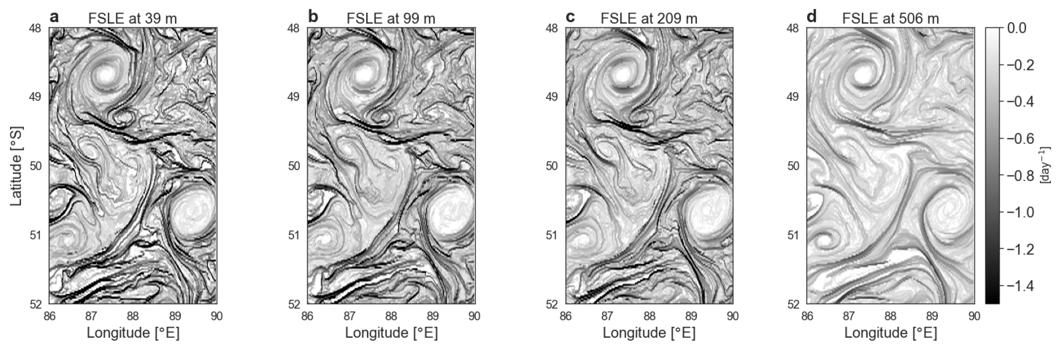
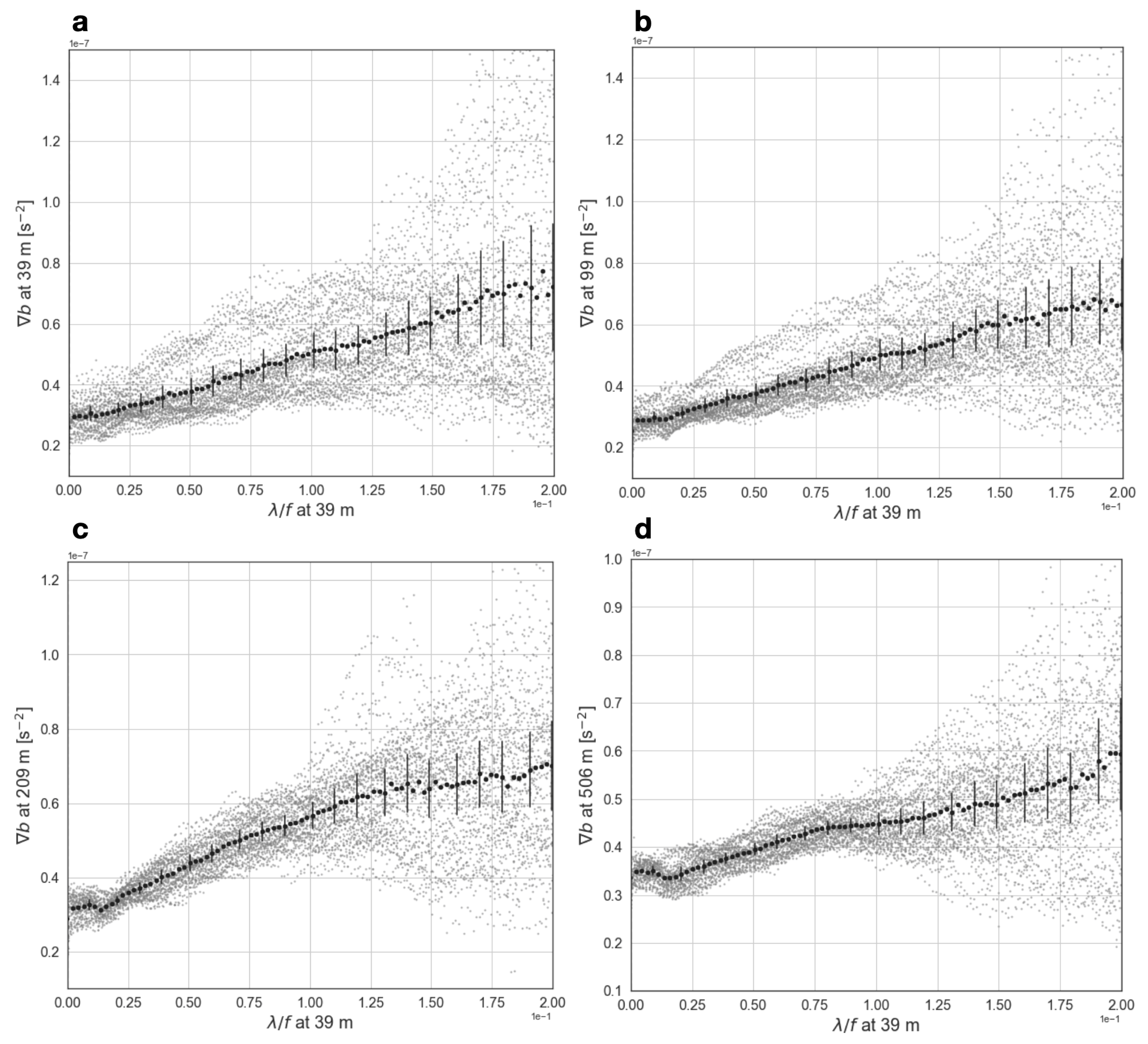
3.3. Recovering Frontal Dynamics at Depth from Finite-Size Lyapunov Exponent at the Surface

Figure 6 presents FSLE computed from the full model horizontal velocity at different depths. FSLE are elevated around and in between coherent eddies. FSLE filaments are either strongly curved over a small region, typically around sub-mesoscale eddies, or weakly curved over a large region, typically in between mesoscale eddies (Figure 6). This is especially true near the surface (Figure 6a). FSLE associated with sub-mesoscale eddies are shallow and vanish at depth, whereas those associated with mesoscale eddies are deep and persist down to depths of at least 500 m (Figure 6b–d), consistent with the fact that energetic eddies are essentially captured by the first baroclinic mode [33,34].
A key question that arises is how to identify the part of the strain field that drives the formation of sub-mesoscale buoyancy fronts at the surface and at depth. In other words, is it the mesoscale (50–300 km) or the sub-mesoscale (<50 km) part of the flow that controls the creation of buoyancy fronts? One way to answer this question is to compute the ratio between the strain rate at a given scale and the strain rate at larger scales, as done in Foussard et al. [35]. This ratio can be expressed as:
R k = k / 2 k l 2 E ( l ) d l k m i n k l 2 E ( l ) d l ,
with k the wavenumber and E ( k ) the velocity spectrum. The numerator represents the strain rate associated with eddies of wavenumber k and the denominator captures the strain rate associated with larger eddies [35,36]. Regardless of depth, R k is close to 1 for k 10 2 cpkm but quickly decreases for smaller length-scales (larger k) and reaches a plateau or a local minimum at length-scales of ∼20 km (Figure 7). This indicates that only scales larger than 20 km impact the stirring of buoyancy anomalies [35,36].
New FSLE are now computed from the model horizontal velocities after application of a low-pass filter with a cutoff wavelength of 20 km on u and v (see Appendix C for more details on the filter). These FSLE capture the part of the flow that contributes to the stirring of buoyancy anomalies, based on the analysis carried in the previous paragraph (Figure 7). They will exclusively be used in the rest of this section and are referred to as FSLE f i l t . FSLE f i l t look alike at all depths both in terms of magnitude and co-location in physical space (Figure 8a–d). More quantitatively, FSLE f i l t at 39 m versus at 209 m and 506 m follow a 1-1 relationship (Figure 9). This highlights the good correspondence between FSLE f i l t at the surface and at depth, and thus the homogeneity of the stirring properties of the flow down to at least 506 m. A sensitivity analysis indicates that the correlation between FSLE f i l t near the surface and at depth decreases when scales smaller than 20 km are included (not shown).
Figure 8 (top and bottom panels) reveal the strong similitude between patterns of FLSE f i l t and | b | : both quantities are elongated and/or curved over ten of kms in the same direction. Furthermore, strong | b | values are almost collocated with strong FSLE f i l t , expect at 506 m where the relationship seems to break down. This may be because at 506 m (i.e., below the permanent thermocline), IGWs have a signature on | b | (Figure A2i and Figure 8h) but they are not correlated with the horizontal velocity gradients. A simple reason explaining this regime shift could be that the depth of the permanent thermocline is set by the depth of the winter mixed layer. Figure 10 confirms the overall similitude between patterns of FLSE f i l t and | b | . It emphasizes that FSLE f i l t and | b | are statistically collocated. Since they are elongated and/or curved over long distances, this result indicates they have statistically the same orientation. These results are consistent with the empirical relation obtained in Siegelman et al. [3], although FSLE from the model have a stronger magnitude than those in Siegelman et al. [3] derived from altimetry. This is due to the different spatial and temporal resolution of both velocity fields (hourly and at 1/48 in the model versus daily and at 1/4 in the altimetry product). These findings suggest that strong | b | , both at the surface and in the ocean interior, are preferentially located in regions of intense surface FSLE, i.e., in regions of strong velocity gradients.
However, one caveat needs to be mentioned. There is a dispersion in the scatter plots of | b | and FSLE f i l t (Figure 10), which can be explained by the phase-lag observed in physical space between the two quantities (Figure 1c). However, even in the presence of a spatial lag, the present results indicate that b is aligned with its neighboring FSLE f i l t (Figure 1c and Figure 8).
In summary, these numerical results demonstrate that the stirring properties of buoyancy gradients at every depth, i.e., the growth rate and orientation of these gradients (explained by the characteristics of the 3D velocity gradient tensor A , see Equations (3) and (4)), can be inferred from surface velocity fields in high EKE regions, characterized by N / f 60 . It suggests that altimetry data can be used to improve the diagnosis of deep-reaching sub-mesoscale dynamics, as discussed in the next section.

4. Application to In Situ Data

Building upon the numerical results of Section 3, we use FSLE and surface geostrophic currents diagnosed from satellite altimetry observations to refine the analysis of sub-mesoscale-resolving in situ observations. The goals of this section are to (i) retrieve the correct orientation, magnitude and growth rate of b observations, and (ii) derive their associated vertical velocities. Indeed, when a sampling device does not perpendicularly cross a front, it leads to an underestimation of the front’s magnitude [1,3].
To achieve (i) and correct for the sampling orientation, the observed buoyancy gradients b x , with x the curvilinear abscissa along the instrument’s trajectory, are normalized as follows:
b x norm = b x sin ( | γ θ | ) ,
with γ the angle between the instrument’s trajectory and the x-axis of the Cartesian coordinate system and θ the angle given by the eigenvector associated with the FSLE eigenvalue λ , which is used to retrieve the orientation of the front with assumptions (see Figure A1 and Appendix A). Equation (6) orients b x norm in the cross-front direction (with x now the cross-front direction) and adjusts its magnitude. As discussed in the preceding section and in Appendix A, the resulting growth rate of b x norm is equal to:
1 b x norm d b x norm d t = u x norm ,
with u norm the cross-front horizontal velocity, x the cross-front direction and u x norm the cross-front velocity gradient (i.e., x u norm ). u x norm is estimated from geostrophic surface currents (u and v) derived from satellite altimetry rotated in the frontal coordinate system by θ (given by the FSLE’s eigenvector, see Appendix A). Note that this method differs from the one developed in Siegelman et al. [3]. Indeed, Siegelman et al. [3] only normalized buoyancy gradients associated with λ > 0.15 day 1 and u x norm was approximated by λ along the instrument’s trajectory in Equation (7). However, λ underestimates the gradients’ growth rate [13], which is more accurately given by Equation (7) [11,32,37] (see also Appendix A).
In the frontogenesis framework, the emergence of vertical velocities counterbalances the formation of sharp sub-mesoscale fronts generated by the velocity gradients (Equation (3)). This equilibrium is captured by the classical omega equation [16]. Thanks to the normalization performed in Equation (6), we can achieve (ii) by using a 2-D (x,z) QG version of the omega equation to compute vertical velocities w, with x the cross-front direction (see methods for more details on the choice of this equation). We recall the 2-D QG omega equation:
N 2 w x x + f 2 w z z = 2 ( u x norm b x norm ) x ,
with u x norm the cross-front horizontal velocity gradient, N the mean Brunt-Väisälä frequency that depends only on z and b x norm the normalized buoyancy gradient. N is estimated from the in situ measurements.
We solve Equations (6) and (8) using a newly available dataset collected by a southern elephant seal east of the Kerguelen plateau in the same season and area as the one studied in Section 3. The transect of interest (in color in Figure 11) has the particularity of sampling several co-interacting mesoscale eddies. As a result, the seal crosses multiple sub-mesoscale fronts that are located at the periphery and in between the mesoscale eddies. The seal’s trajectory is often oblique rather than perpendicular to the FSLE’s orientation, which makes it an ideal case study to evaluate the impact of our method.
At latitudes of 50 S, Sea Surface Height (SSH) products distributed by AVISO have an effective resolution of ∼100 km [38], i.e., not fine enough to recover the part of the horizontal velocity field in the range 20–100 km identified in the previous section as being active in the production of frontogenesis-induced b (Figure 7). Indeed, vorticity, strain rate and the Okubo-Weiss quantity derived from SSH are pixel-like and do not allow the identification of sub-mesoscale fronts and filaments (Figure 11a–c). However, it is possible to recover scales in the 20–100 km range with the FSLE value-added product distributed by AVISO (Figure 11d). This is because, in the Lagrangian advection framework, fine scales are created through time as a result of the direct cascade of potential energy [11]. FSLE derived from altimetry exhibit filamentary structures that are not present in the other quantities (Figure 11). FSLE’s magnitude broadly coincide with the background strain rate’s magnitude (Figure 11b,d). In regions of strong strain, i.e., when the Okubo-Weiss quantity is positive (in red in Figure 11c), FSLE are elevated. Note that as in the model results, FSLE are an order of magnitude lower than strain and vorticity. Hence, from these observations and the theoretical arguments developed in Appendix A, it appears necessary to know both the FSLE’s eigenvector and the velocity gradients to recover the orientation and growth rate of buoyancy gradients, respectively.
The impact of the normalization (Equation (6)) is significant (Figure 12). On average, | b | are 1.8 times larger after normalization and can be as much as 4 times larger (at 1330 km in Figure 12c). This highlights the usefulness of incorporating the FSLE’s orientation into the analysis of sub-mesoscale-resolving datasets. The section sampled by the seal shares a lot of common features with the section from the model (Figure 2). Lateral gradients of buoyancy ( b x norm ) are located in between and on the border of mesoscale eddies. They are slanted and follow isopycnals (at 1300–1370 km in Figure 12b) or the MLD (at 1050–1090 km in Figure 12b). b x norm extend at depth down to at least 500 m, highlighting the presence of energetic submesoscales in the ocean interior. Similar to the model, the signature of IGWs is noticeable at the base of the mixed layer, where b x norm are organized in thin vertical bands of alternating sign (at ∼1100 km in Figure 12b). The inverse Richardson number, defined as Ri 1 = f 2 N 2 / b x norm 2 , assuming thermal wind balance, is of order one at the location of strong b x norm (not shown), similar to what is found in the model and in other in situ observations from 2014 in the same area and season [3]. This suggests an energetic ageostrophic regime associated with an elevated growth rate of buoyancy gradients and intense vertical velocities w [5]. As mentioned above, using the growth rate u x n o r m instead of λ (as done in Siegelman et al. [3]) makes a considerable difference. Indeed, λ consistently underestimates u x n o r m (Figure 13), which should then impact the vertical velocities’ magnitude, as investigated below.
Vertical velocities are presented in Figure 14. In the first panel, Equation (2) is solved in the along-track direction, i.e., with x the curvilinear abscissa along the seal’s track. This equation involves b x and u x along the seal’s path and yields w (Figure 14a). In the second panel, Equation (8) is now solved in the cross-front direction. This is equivalent to changing the orientation of the fronts along the seal’s trajectory such that the fronts are perpendicular to this trajectory (or, equivalently, changing locally the seal’s trajectory such that this trajectory is perpendicular to the fronts). This equation involves b x norm and u x norm cross-front and yields w n o r m (Figure 14b). Finally, the third panel shows the ratio between w n o r m and w (Figure 14c). Consistent with the buoyancy gradient’s normalization (Figure 12), computing vertical velocities in the cross-front direction instead of in the along-track direction makes a significant difference. On average, w n o r m is 2.15 times larger than w and can be as much as 15.6 times larger (at 180 m depth/1335 km in Figure 14) for w > 20 m day 1 . Even though the sign of the vertical velocity rarely changes between w n o r m and w, instances where it does (in blue in Figure 14c), as well as instances where w are overestimated compared to w n o r m (i.e., when 0 < w n o r m / w < 1 ), further highlight the importance of considering the horizontal velocity field in the frontal coordinate system. The vertical section of w n o r m reveals positive and negative values with large magnitudes of hundreds of meters per day (Figure 14b), i.e., an order of magnitude greater than what is attributed to mesoscale eddies alone [39]. Vertical velocities have a width of 5 to 10 km. They are intensified in the ocean interior, below the mixed layer down to at least 500 m. Large values of w are collocated with strong buoyancy gradients, and are therefore mostly found on the edges of, and in between, eddies. The vertical velocity field is coherent over a few dives, suggesting that IGWs do not contribute to it. Around 1100 km for example, the signature of IGWs is noticeable on buoyancy gradients below the MLD (Figure 12b) but vertical velocities are weak (Figure 14b). This is consistent with the physics captured by the omega equation, in the sense that b due to IGWs are not necessarily correlated with velocity gradients and hence do not contribute to the vertical velocity field derived from the omega equation [17]. In addition, IGWs are known to impact buoyancy gradients when N / f 300 [40], which is not the case here as N / f 60 .
Note that compared to the Sawyer Eliassen equation [41], there is a tendency for w diagnosed here to be underestimated by ∼1.4 [3]. However, the validity of using the omega equation to reconstruct the vertical velocity field has been explored by numerous studies [42,43] (see in particular Figure 3 in Qiu et al. [43]) and a comparison with w from the model is presented in the supplementary material of Siegelman et al. [3]. Applying the same methodology to a synthetic trajectory extracted from the model would also be valuable to pursue in future work.

5. Discussion

in situ CTD observations at high-resolution can now be acquired by numerous platforms, including ocean/sea glider, shipboard-ADCP, SeaSoar, saildrone or animal-borne instrument [1,2,3,4,6]. Resulting 2-D (xz) sections often reveal numerous sub-mesoscale fronts extending down to ∼500 m, especially in high EKE regions, that are characterized by high Rossby and low Richardson numbers. It emphasizes their energetic dynamics, which includes vertical velocities. As such, it has been suggested that these fronts considerably impact oceanic vertical transport [6]. However, inferring their dynamics requires knowledge of the past evolution of the 3-D structure of the horizontal velocity field over a few days, which is rarely accessible from high-resolution in situ data. To meet this challenge, we use a numerical simulation that includes numerous deep-reaching fronts associated with Rossby and Richardson numbers of order one. Results demonstrate that it is possible to recover the correct orientation, magnitude and growth rate of b observations at depth from FSLE’s orientation at the surface. In turn, this enables the inference of deep-reaching frontal dynamics in terms of vertical velocities.
However, the present study solely considers a region of high EKE of the ACC [19] characterized by N / f 60 , in springtime. This area might not be characteristic of the entire ACC in terms of EKE and vertical stratification, nor of other seasons (e.g., in winter one can expect submesoscales to be more energetic [6,44]). As such, these findings call for extended analyses at different seasons and throughout the world oceans to explore the generic character of our results.
However, based on the present numerical results, we propose a two-step procedure for the analysis of existing sub-mesoscale-resolving dataset using satellite altimetry observations:
A1.
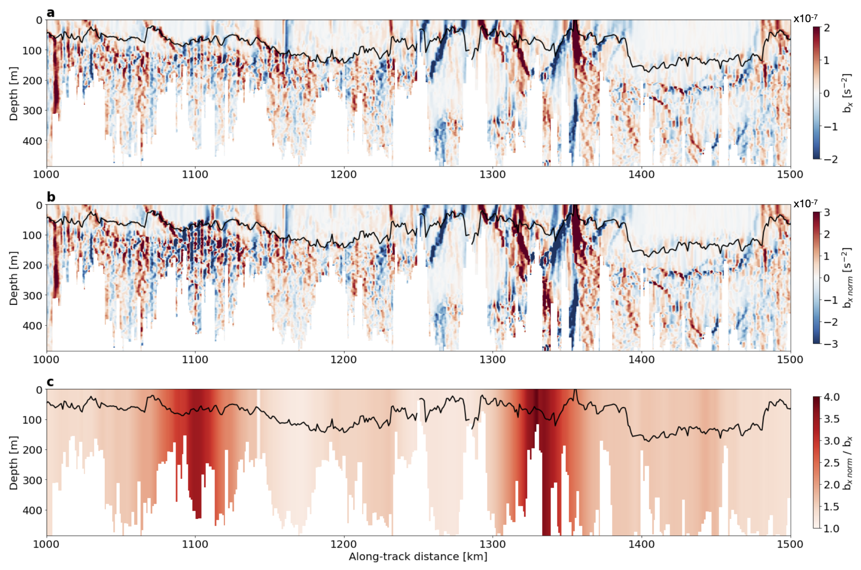
We recover the orientation of sampled lateral buoyancy gradients, and subsequently their correct magnitude through a normalization scheme. This normalization takes into account the angle between the sampling platform and the front’s orientation deduced from the FSLE’s eigenvector.
A2.
We diagnose vertical velocities from the normalized lateral buoyancy gradients using a 2-D QG version of the omega equation.
A weakness of step A1. is that it fails when the platform moves in the along-front direction. In this case, the sine of the angle between the front and the platform is close to 0, which may lead to spurious normalized values. Furthermore, as mentioned in the main text, the QG omega equation used in step A2. underestimates vertical velocities (see supplementary information in Siegelman et al. [3] for a discussion).
Results of the present study can also be applied to the planning of in situ experiments, using satellite altimetry data in real time to design an optimal sampling strategy of sub-mesoscale ocean fronts. We would like to suggest the following strategy, intended for ship-board instruments or remote piloting of an ocean robot:
B1.
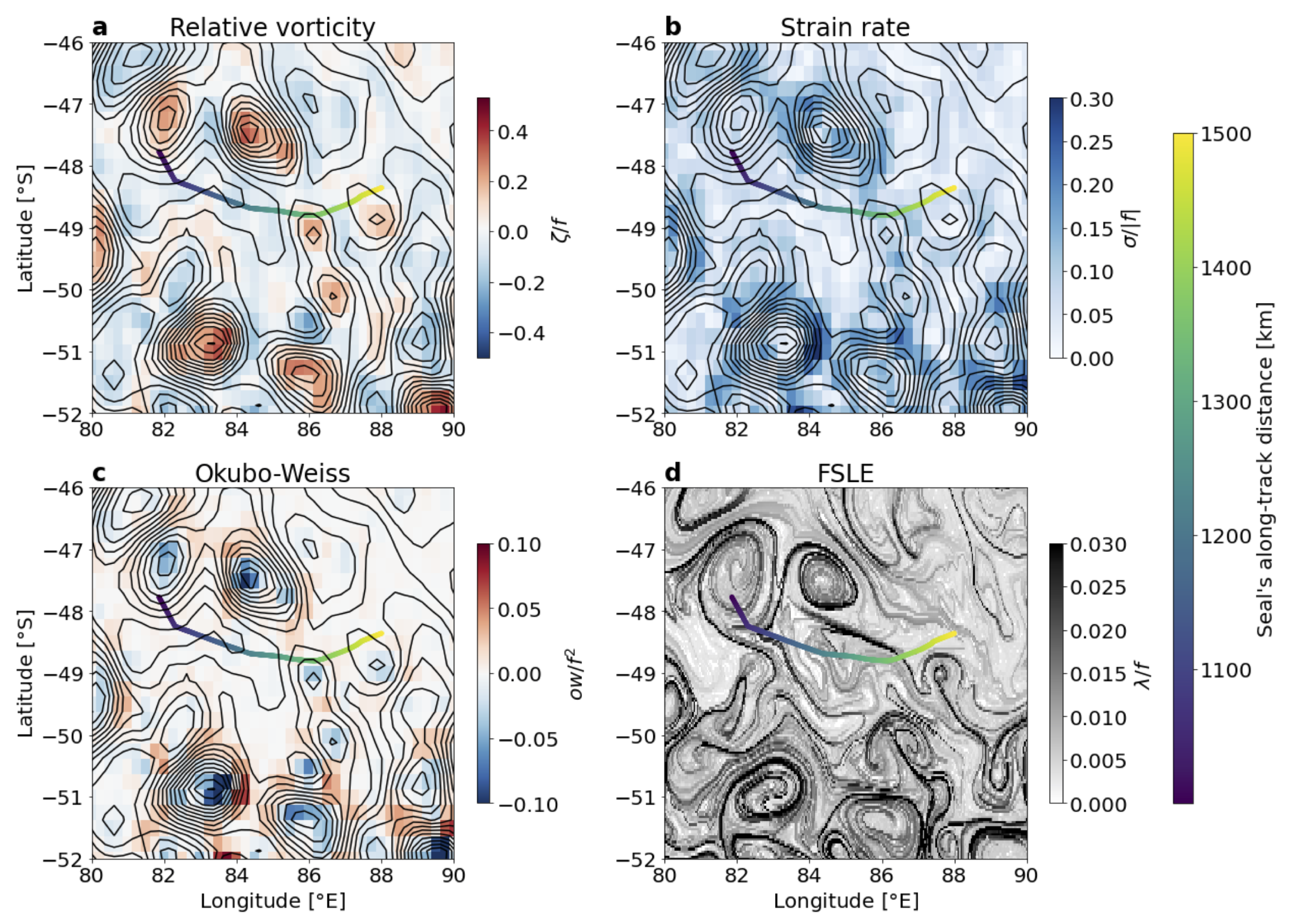
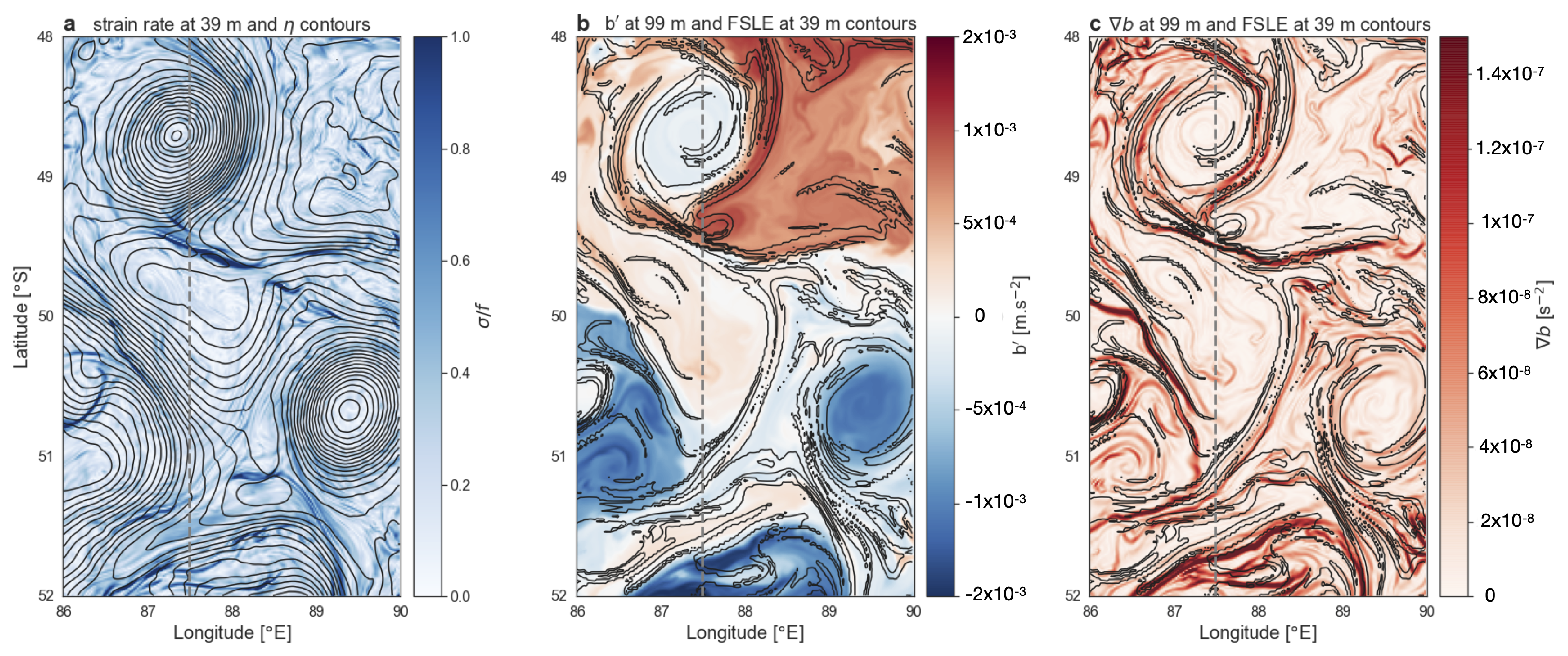
Identify areas of strong background strain from near-real time satellite observations of geostrophic currents (i.e., when the Okubo-Weiss quantity is positive, Figure 11c).
B2.
Use near-real time AVISO-FSLE products to identify the location and orientation of FSLE filaments (Figure 11d).
B3.
Pilot the ship/robot perpendicular to this orientation. One should then perpendicularly cross sub-mesoscale fronts embedded in the background flow.
Note that even though mesoscale eddies evolve slowly compared to sub-mesoscale fronts, their geometry, and therefore stirring properties, can change on timescales of O(day) as mentioned in Appendix A. As a result, FSLE vary quickly in time and their maxima can move from a quarter of a degree in just two days (see for example at 50.75 S and 51 S in Figure 15). As such, it is important to use near-real time FSLE distributed by AVISO in step B2. When possible, we encourage users to compute their own FSLE from near-real time SSH observations as near-real-time FSLE are provided by AVISO with a 20-day delay. In addition, while this method is viable for a ship that travels ≥ 200 km/day, it is not suitable for every instrument. For instance, gliders only travel ∼ 20 km/day so the features are evolving at scales that make it difficult to achieve this planning.
Step B3. accounts for the potential co-location mismatch between b and FSLE, despite their common alignment. Indeed, the position of a large FSLE filament is not necessarily indicative of the presence of a deep sub-mesoscale front at this exact location, but rather, of the presence of one or several fronts in its vicinity, that are aligned with the FSLE’s orientation (Figure 1c). As such, repeating long-enough transect perpendicular to the FSLE’s orientation should enable the crossing of several sub-mesoscale fronts at an angle of 90 (for example ∼50 km-long transects separated by ∼10 km each). Furthermore, the sampling time should take into account the synoptic scale associated with the time evolution of the mesoscale field’s geometry (O(day)), and ideally each transect should be collected in less than ∼10 h. This method appears well suited for deep-reaching sub-mesoscale fronts that are elongated over tens of kilometers (a variant of which has been successfully used in Legal et al. [45]) but a potential drawback is that it may fail for shorter and smaller fronts, such as those present within the mixed layer.
Results of this study should gain increasing utility in the context of upcoming satellite missions, such as SWOT or WACM, that will provide high-resolution observations of the surface currents on a global scale. These future observations should help refine our results and eventually extend them to smaller scales. Given the recent technological advances in in situ sampling, sub-mesoscale-resolving datasets are expected to become increasingly available such that the approaches proposed here should have increasing utility (e.g., the upcoming S-MODE experiment).

Author Contributions

Methodology, L.S. and P.K.; formal analysis, L.S., P.K.; writing—original draft preparation, L.S., P.K. and A.F.T.; writing—review and editing, L.S., P.K., A.F.T., H.S.T., D.M.; numerical simulation, D.M., H.S.T. All authors have read and agreed to the published version of the manuscript.

Funding

L.S., H.S.T. and D.M. carried research at the Jet Propulsion Laboratory, California Institute of Technology, under a contract with NASA with support from the Physical Oceanography (PO) and Modeling, Analysis, and Prediction (MAP) Programs. L.S. is a NASA-JVSRP affiliate and is supported by a Caltech-JPL postdoctoral fellowship. P.K. is supported by a NASA NPP Senior Fellowship and by the SWOT and S-Mode projects. A.F.T. is supported by the David and Lucille Packard Foundation and NASA grant NNX16AG42G.

Acknowledgments

High-end computing resources for the numerical simulation were provided by the NASA Advanced Supercomputing (NAS) Division at the Ames Research Center. Thanks to Christopher Henze at NASA Ames Hyperwall and MITgcm developers and NAS scientists that made available the model outputs. This work was supported by the CNES-TOSCA project Elephant seals as Oceanographic Samplers of sub-mesoscale features led by C. Guinet with support of the French Polar Institute (Programs 109 and 1201). Thanks to Fabien Roquet and Baptiste Picard that made available the seal’s data.

Conflicts of Interest

The authors declare no conflict of interest.

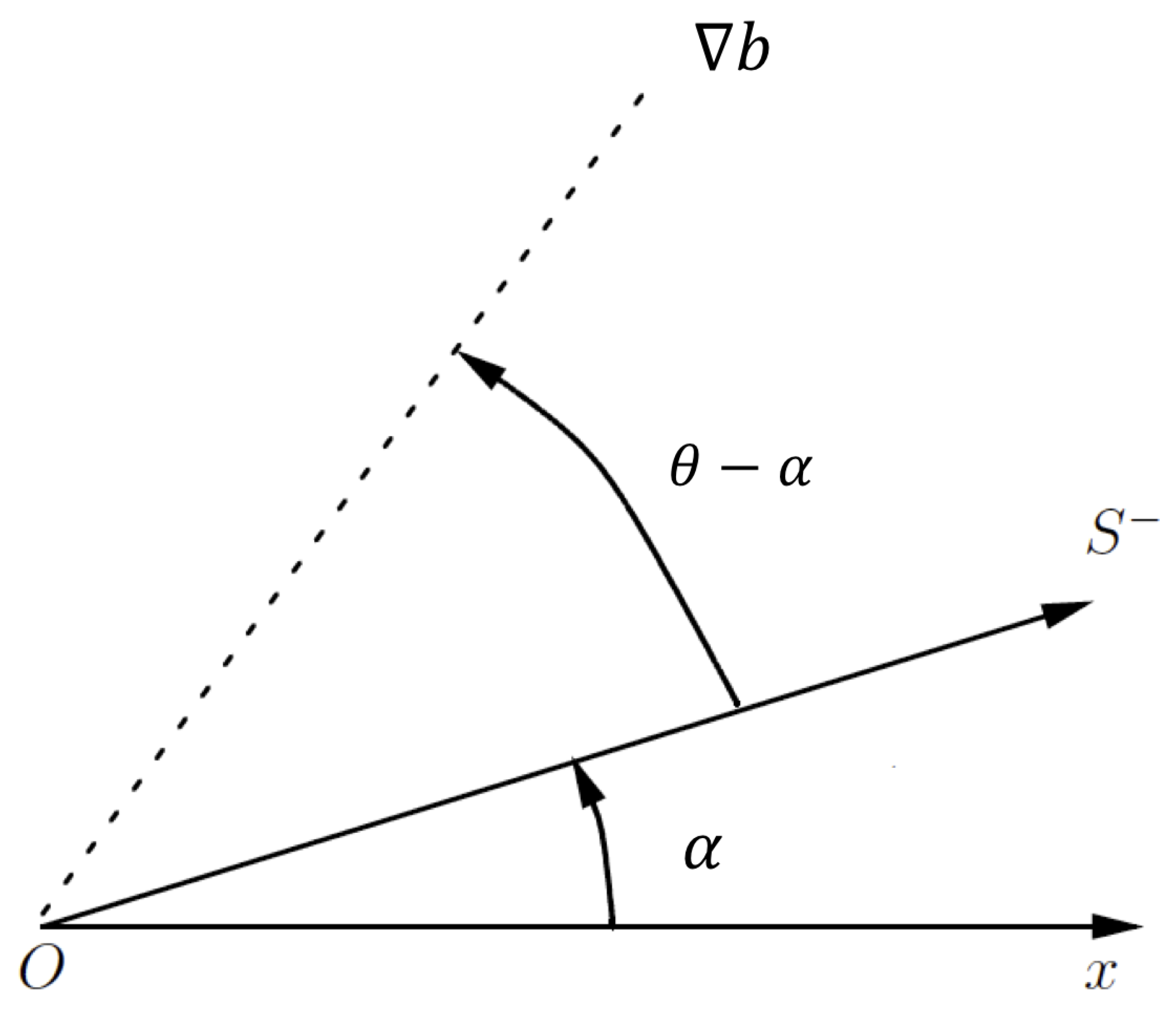
Appendix A. On the Growth Rate and Orientation of Buoyancy Gradient

As mentioned in the main text, the time evolution of a buoyancy gradient is given by:
d b d t = A b N 2 w ,
with b the lateral buoyancy gradient, w the vertical velocity field, N 2 the vertical stratification and A the velocity gradient tensor, defined as:
A 1 2 σ n σ s + ζ σ s ζ σ n ,
with ζ = x v y u the relative vorticity, σ n = x u y v the normal strain rate, and σ s = x v + y u the shear strain rate [29].
From Equation (A1), one can see that the growth of b depends on the eigenvalues of A . A commonly used criterion to infer the production of b is the Okubo-Weiss quantity (W), derived by Okubo [30] and Weiss [46,47]. W is the squared eigenvalues of A:
W = 1 4 ( σ n 2 + σ s 2 ζ 2 ) .
The Okubo-Weiss quantity is used in Section 3 to partition the fluid into elliptic regions dominated by ζ , and hyperbolic regions dominated by σ n and σ s . Hyperbolic regions coincide with an excess of the magnitude of strain over vorticity and conversely for elliptic ones. Under the assumption that the velocity gradient is slowly varying along a Lagrangian trajectory, the behavior of b can be determined by W: | b | do not grow in vortex cores where W < 0 since the eigenvalues of A are purely imaginary. In this case, the gradient vector experiences a simple rotation. On the other hand, in strain-dominated areas where W > 0 , the eigenvalues of A are real and | b | exponentially grow. Thus, strain-dominated areas are particularly prone to the formation of sub-mesoscale fronts. These mechanisms are further detailed in many studies [32,48,49,50,51] and we summarize some of them below.
The asymmetric part of A is explained by the relative vorticity whose effect is only to rotate b . The symmetric part is explained by the strain field whose effects are (i) to align b toward the compressional strain direction (one of the eigenvectors of the symmetric part of A ) and (ii) to increase the magnitude of b with a maximum growth rate equal to σ = σ n 2 + σ s 2 . Using ( σ n , σ s ) = σ ( sin ( 2 ϕ ) , cos ( 2 ϕ ) ) , the compressional strain direction has an angle with the x-axis equal to α = ϕ π / 4 [32] (Figure A1). Using b = | b | ( cos ( θ ) , sin ( θ ) ) , with θ the angle between b and the x-axis (Figure A1), and ignoring w, the growth and alignment properties of b are given by [32]:
1 | b | d | b | d t = σ 2 cos 2 ( θ α ) ,
d ( θ α ) d t = σ ζ + d ϕ / d t σ sin 2 ( θ α ) ,
with d ϕ / d t the rotation of the strain axis along a Lagrangian trajectory, which has a typical magnitude of ζ [31,32]. Thus, from Equation (A4), the growth rate of b is σ cos ( 2 ( θ α ) ) [32]. The typical time scale for θ α to reach a steady state is of the order of σ 1 (i.e., O(day)) [32]. Equation (A5) means that in most cases, the orientation of b ( θ ) differs from the orientation of the strain compressional axis ( α ). The growth rate and orientation of tracer gradients given by Equations (A4) and (A5) have been validated using numerical simulations with high resolution [32,37].
Figure A1. θ is the angle between b and the x-axis and α is the angle between the compressional strain vector ( S ) and the x-axis.
Fluids 05 00145 g0a1
Integrating Equation (A5) to get b -orientation requires knowledge of the time evolution of A . A simpler method to get θ is to estimate FSLE that implicitly use the same information for the velocity field [11,12,13]. Equation (A4) can then be used to estimate the growth rate of b from satellite observations. Indeed, in addition to θ diagnosed from FSLE (using satellite observations), α and σ can be retrieved from the strain components estimated from surface geostrophic currents (diagnosed from altimetry) via α = 1 2 arctan ( σ s σ n ) and σ = σ n 2 + σ s 2 . However, the growth rate of b can be further simplified if expressed in terms of the velocity field in the Cartesian frame associated with b ’s orientation. Indeed, using the definition of σ n and σ s , the growth rate in Equation (A4) can be written as:
G R = σ 2 cos 2 ( θ α ) = 1 2 2 x u cos 2 θ + ( x v + y u ) sin 2 θ .
with GR the growth rate. Then, when the Cartesian frame of reference, as well as the velocity field, are rotated by θ , the growth rate becomes:
G R = u x norm ,
with u norm the cross-front horizontal velocity, x the cross-front direction and u x norm (i.e., x u norm ) the cross-front velocity gradient. The growth rate given by Equation (A7) is the one used in Section 4 (Equation (7)). Note that a more accurate estimation of the growth rate has been proposed by previous studies [31,52]. This estimation is based on the Lagrangian acceleration that drive the time evolution of the velocity field [31] and, consequently, explicitly takes into account the time evolution of the strain field σ . However, because of the assumptions considered in this study and in particular the use of only a 2-D quasi-geostrophic Omega equation, we have chosen the simplest estimation of the growth rate, i.e., the one given by Equations (A6) and (A7).

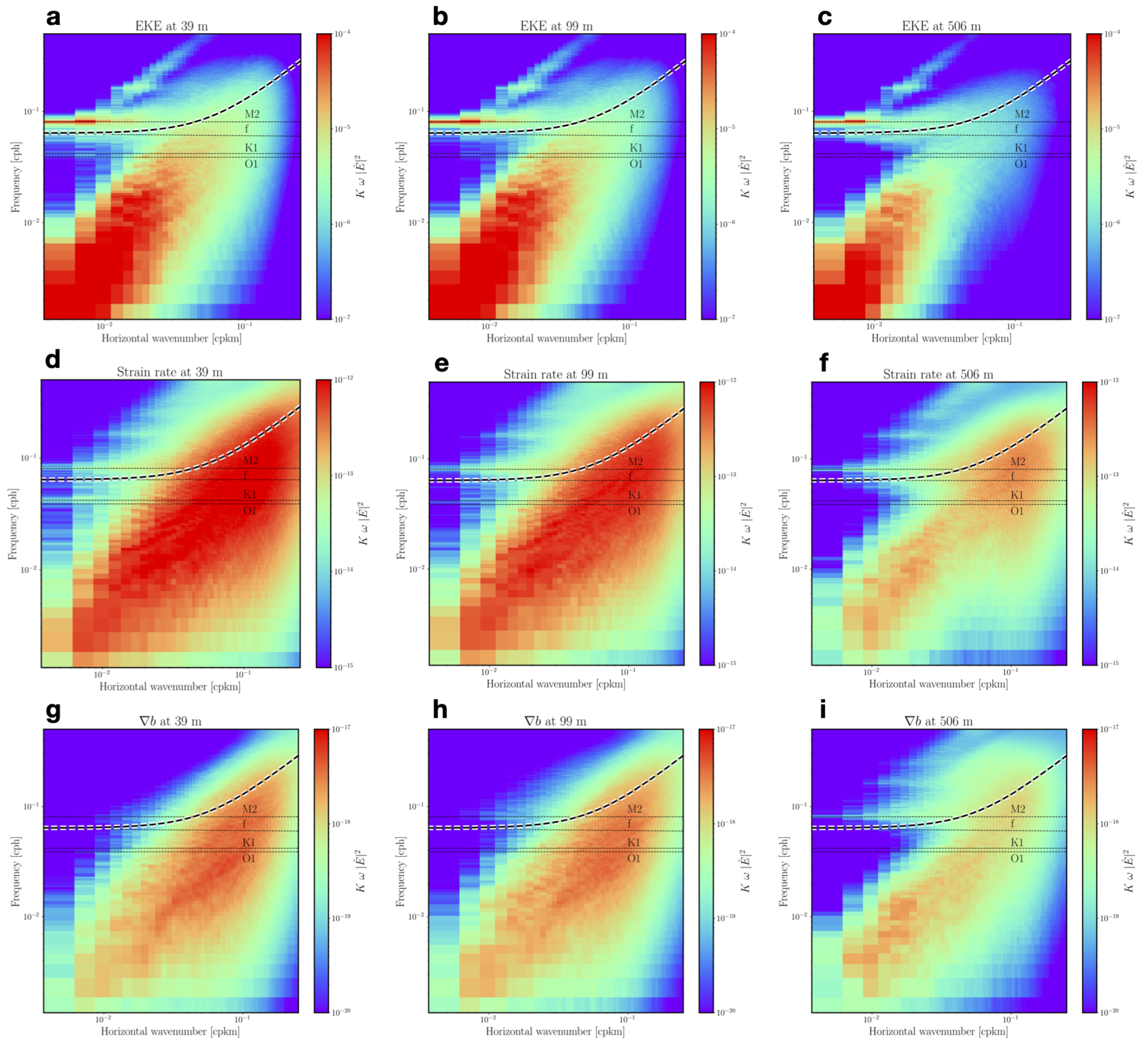
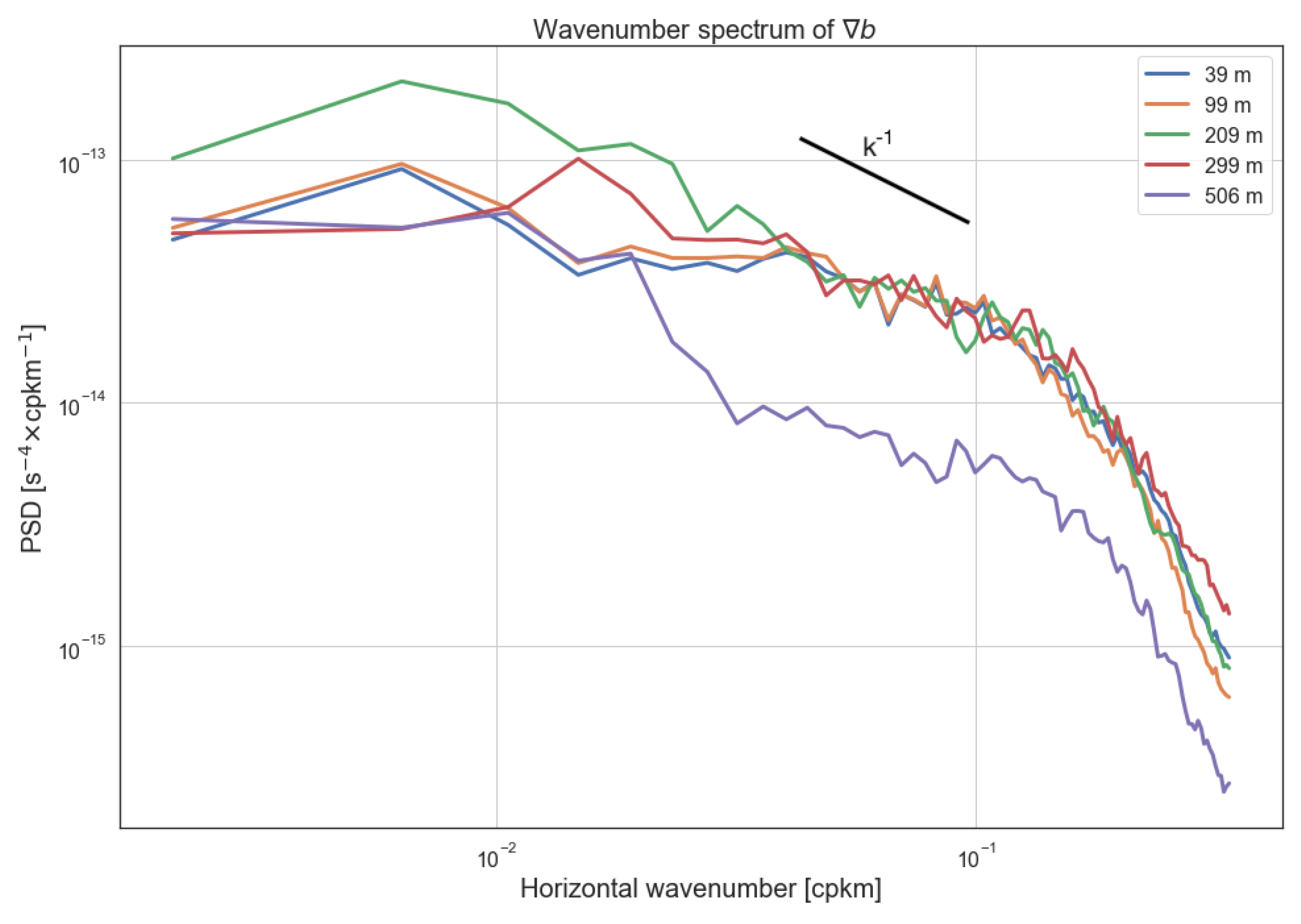
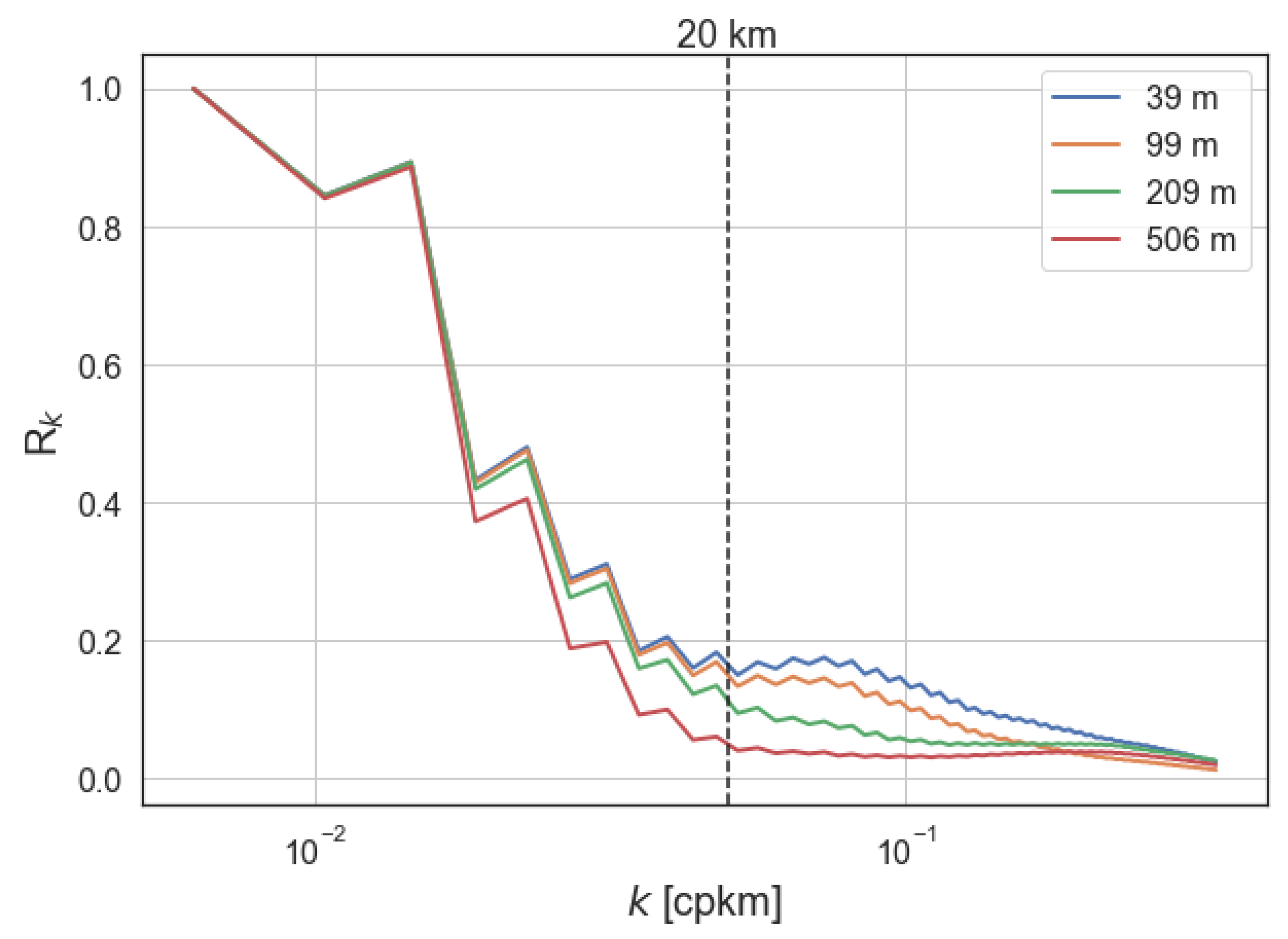
Appendix B. Frequency-Wavenumber Spectrum

We refer the reader to [9] for the methodology used to compute ω -k spectrum. Figure A2 shows ω -k spectra of KE, strain rate and | b | at 39 m, 99 m and 506 m computed in the study area from 27 October to 27 December 2011. They have a similar shape from the surface down to 506 m. As expected, most of the KE is contained at mesoscale (>50 km) and low frequencies (Figure A2a–c). The relative contribution of IGWs is weak compared to that of balanced motions. The strain rate and | b | exhibit a different distribution with a large part of the variance contained at submesoscales (<50 km, Figure A2d–i). Above 506 m, strain rate and | b | are only weakly affected by linear IGWs (above the dashed line), whereas at 506 m the impact of linear IGWs is proportionally greater. Overall, the ω -k spectra indicate that the contribution of submesoscales ( 50 km) to the strain rate and to b is significant and that linear IGWs have a weak impact away from the seasonal and permanent thermocline. These results emphasize the existence of energetic submesoscales in the ocean interior.
Figure A2. Frequency-wavenumber spectra computed from October 27 to December 27, 2011 of (a) KE at 39 m, (b) KE at 99 m, (c) KE at 506 m, (d) Strain rate at 39 m, (e) Strain rate at 99 m, (f) Strain rate at 506 m, (g) | b | at 39 m, (h) | b | at 99 m, (i) | b | at 506 m. The dashed line corresponds to the dispersion relation curve (associated with linear internal gravity waves, IGWs) that corresponds to the highest baroclinic mode resolved by the simulation. This curve allows for the partition between balanced motions (below the curve) and IGWs (above the curve). These spectra are presented in a variance preserving form, which allows the direct comparison of the relative contribution of different time and spatial scales to the total variance.
Fluids 05 00145 g0a2

Appendix C. Filter Cutoff Wavelength

A 2-D Gaussian smoother filter is applied isotropically to the model horizontal velocities field with a cutoff wavelength λ c = 20 km. This filter is thoroughly described in Appendix C of Chelton et al. [53]. However, briefly, the 2-D weighting function for isotropic smoothing can be expressed as
w 2 d ( x , y ) = w 2 d ( r ) ,
where r = ( x 2 + y 2 ) 1 / 2 is the radial distance from the estimation location to each data point within the 2-D span of the smoother. Here, we use a Gaussian-weighted smoother for which the weighting function in one dimension is
w G ( x ) = 1 π L G e x 2 / L G 2 ,
where L G defines the e-folding scale of Gaussian weighting. The normalization factor π L G constrains the weighting function (A9) to have unit area, as required for unbiased smoothing. The parameter L G of the Gaussian smoother (A9) is related to the desired half-power filter cutoff wavenumber k c and associated wavelength λ c = k c 1 by
L G = ln ( 0.5 ) 2 π 2 1 / 2 1 k c = 0.187 λ c .

References

  1. Thompson, A.F.; Lazar, A.; Buckingham, C.; Naveira Garabato, A.C.; Damerell, G.M.; Heywood, K.J. Open-ocean submesoscale motions: A full seasonal cycle of mixed layer instabilities from gliders. J. Phys. Oceanogr. 2016, 46, 1285–1307. [Google Scholar] [CrossRef] [Green Version]
  2. Yu, X.; Naveira Garabato, A.C.; Martin, A.P.; Buckingham, C.E.; Brannigan, L.; Su, Z. An annual cycle of submesoscale vertical flow and restratification in the upper ocean. J. Phys. Oceanogr. 2019, 49, 1439–1461. [Google Scholar] [CrossRef]
  3. Siegelman, L.; Klein, P.; Rivière, P.; Thompson, A.F.; Torres, H.S.; Flexas, M.; Menemenlis, D. Enhanced upward heat transport at deep submesoscale ocean fronts. Nat. Geosci. 2020, 13, 50–55. [Google Scholar] [CrossRef]
  4. Siegelman, L. Energetic submesoscale dynamics in the ocean interior. J. Phys. Oceanogr. 2020, 50, 727–749. [Google Scholar] [CrossRef] [Green Version]
  5. Thomas, L.N.; Tandon, A.; Mahadevan, A. Submesoscale processes and dynamics. Ocean. Model. Eddying Regime 2008, 177, 17–38. [Google Scholar]
  6. Su, Z.; Wang, J.; Klein, P.; Thompson, A.F.; Menemenlis, D. Ocean submesoscales as a key component of the global heat budget. Nat. Commun. 2018, 9, 775. [Google Scholar] [CrossRef] [Green Version]
  7. Marshall, J.; Adcroft, A.; Hill, C.; Perelman, L.; Heisey, C. A finite-volume, incompressible Navier Stokes model for studies of the ocean on parallel computers. J. Geophys. Res. Ocean. 1997, 102, 5753–5766. [Google Scholar] [CrossRef] [Green Version]
  8. Hill, C.; Menemenlis, D.; Ciotti, B.; Henze, C. Investigating solution convergence in a global ocean model using a 2048-processor cluster of distributed shared memory machines. Sci. Program. 2007, 15, 107–115. [Google Scholar] [CrossRef]
  9. Torres, H.S.; Klein, P.; Menemenlis, D.; Qiu, B.; Su, Z.; Wang, J.; Chen, S.; Fu, L.L. Partitioning ocean motions into balanced motions and internal gravity waves: A modeling study in anticipation of future space missions. J. Geophys. Res. Ocean. 2018, 123, 8084–8105. [Google Scholar] [CrossRef] [Green Version]
  10. d’Ovidio, F.; Fernández, V.; Hernández-García, E.; López, C. Mixing structures in the Mediterranean Sea from finite-size Lyapunov exponents. Geophys. Res. Lett. 2004, 31. [Google Scholar] [CrossRef] [Green Version]
  11. Lapeyre, G. Characterization of finite-time Lyapunov exponents and vectors in two-dimensional turbulence. Chaos Interdiscip. J. Nonlinear Sci. 2002, 12, 688–698. [Google Scholar] [CrossRef] [PubMed] [Green Version]
  12. Keating, S.R.; Smith, K.S.; Kramer, P.R. Diagnosing lateral mixing in the upper ocean with virtual tracers: Spatial and temporal resolution dependence. J. Phys. Oceanogr. 2011, 41, 1512–1534. [Google Scholar] [CrossRef] [Green Version]
  13. Waugh, D.W.; Abraham, E.R. Stirring in the global surface ocean. Geophys. Res. Lett. 2008, 35. [Google Scholar] [CrossRef] [Green Version]
  14. Siegelman, L.; Roquet, F.; Mensah, V.; Rivière, P.; Pauthenet, E.; Picard, B.; Guinet, C. Correction and accuracy of high-and low-resolution ctd data from animal-borne instruments. J. Atmos. Ocean. Technol. 2019, 36, 745–760. [Google Scholar] [CrossRef]
  15. Intergovernmental-Oceanographic-Commission. The International Thermodynamic Equation of Seawater—2010: Calculation and Use of Thermodynamic Properties. [Includes Corrections Up to 31st October 2015]; UNESCO: Paris, France, 2010. [Google Scholar]
  16. Hoskins, B.J.; Draghici, I.; Davies, H.C. A new look at the ω-equation. Q. J. R. Meteorol. Soc. 1978, 104, 31–38. [Google Scholar] [CrossRef]
  17. Giordani, H.; Prieur, L.; Caniaux, G. Advanced insights into sources of vertical velocity in the ocean. Ocean. Dyn. 2006, 56, 513–524. [Google Scholar] [CrossRef]
  18. Burns, K.J.; Vasil, G.M.; Oishi, J.S.; Lecoanet, D.; Brown, B. Dedalus: Dedalus: A flexible framework for numerical simulations with spectral methods. Phys. Rev. Res. 2020, 2, 023068. [Google Scholar] [CrossRef] [Green Version]
  19. Thompson, A.F.; Naveira Garabato, A.C. Equilibration of the Antarctic Circumpolar Current by standing meanders. J. Phys. Oceanogr. 2014, 44, 1811–1828. [Google Scholar] [CrossRef]
  20. Vallis, G.K. Atmospheric and Oceanic Fluid Dynamics; Cambridge University Press: Cambridge, UK, 2017. [Google Scholar]
  21. Haynes, P.; Anglade, J. The vertical-scale cascade in atmospheric tracers due to large-scale differential advection. J. Atmos. Sci. 1997, 54, 1121–1136. [Google Scholar] [CrossRef]
  22. Klein, P.; Treguier, A.M.; Hua, B.L. Three-dimensional stirring of thermohaline fronts. J. Mar. Res. 1998, 56, 589–612. [Google Scholar] [CrossRef]
  23. Meunier, T.; Ménesguen, C.; Schopp, R.; Le Gentil, S. Tracer stirring around a meddy: The formation of layering. J. Phys. Oceanogr. 2015, 45, 407–423. [Google Scholar] [CrossRef] [Green Version]
  24. Hua, B.L.; Haidvogel, D.B. Numerical simulations of the vertical structure of quasi-geostrophic turbulence. J. Atmos. Sci. 1986, 43, 2923–2936. [Google Scholar] [CrossRef] [Green Version]
  25. Smith, K.S.; Ferrari, R. The production and dissipation of compensated thermohaline variance by mesoscale stirring. J. Phys. Oceanogr. 2009, 39, 2477–2501. [Google Scholar] [CrossRef]
  26. Molemaker, M.J.; McWilliams, J.C.; Capet, X. Balanced and unbalanced routes to dissipation in an equilibrated Eady flow. J. Fluid Mech. 2010, 654, 35–63. [Google Scholar] [CrossRef]
  27. Roullet, G.; Klein, P. Cyclone-anticyclone asymmetry in geophysical turbulence. Phys. Rev. Lett. 2010, 104, 218501. [Google Scholar] [CrossRef] [PubMed]
  28. Klein, P.; Lapeyre, G.; Siegelman, L.; Qiu, B.; Fu, L.L.; Torres, H.; Su, Z.; Menemenlis, D.; Le Gentil, S. Ocean-Scale Interactions From Space. Earth Space Sci. 2019, 6, 795–817. [Google Scholar] [CrossRef] [Green Version]
  29. Lapeyre, G.; Klein, P.; Hua, B.L. Oceanic Restratification Forced by Surface Frontogenesis. J. Phys. Oceanogr. 2006, 36, 1577–1590. [Google Scholar] [CrossRef]
  30. Okubo, A. Horizontal dispersion of floatable particles in the vicinity of velocity singularities such as convergences. Deep. Sea Res. Oceanogr. Abstr. 1970, 17, 445–454. [Google Scholar] [CrossRef]
  31. Hua, B.L.; Klein, P. An exact criterion for the stirring properties of nearly two-dimensional turbulence. Phys. D Nonlinear Phenom. 1998, 113, 98–110. [Google Scholar] [CrossRef]
  32. Lapeyre, G.; Klein, P.; Hua, B.L. Does the tracer gradient vector align with the strain eigenvectors in 2D turbulence? Phys. Fluids 1999, 11, 3729–3737. [Google Scholar] [CrossRef] [Green Version]
  33. Smith, K.S.; Vallis, G.K. The scales and equilibration of midocean eddies: Freely evolving flow. J. Phys. Oceanogr. 2001, 31, 554–571. [Google Scholar] [CrossRef] [Green Version]
  34. Lapeyre, G. What vertical mode does the altimeter reflect? On the decomposition in baroclinic modes and on a surface-trapped mode. J. Phys. Oceanogr. 2009, 39, 2857–2874. [Google Scholar] [CrossRef]
  35. Foussard, A.; Berti, S.; Perrot, X.; Lapeyre, G. Relative dispersion in generalized two-dimensional turbulence. J. Fluid Mech. 2017, 821, 358–383. [Google Scholar] [CrossRef]
  36. Scott, R. Local and nonlocal advection of a passive scalar. Phys. Fluids 2006, 18, 116601. [Google Scholar] [CrossRef]
  37. Lapeyre, G.; Hua, B.L.; Klein, P. Dynamics of the orientation of active and passive scalars in two-dimensional turbulence. Phys. Fluids 2001, 13, 251–264. [Google Scholar] [CrossRef] [Green Version]
  38. Ballarotta, M.; Ubelmann, C.; Pujol, M.I.; Taburet, G.; Fournier, F.; Legeais, J.F.; Faugère, Y.; Delepoulle, A.; Chelton, D.; Dibarboure, G.; et al. On the resolutions of ocean altimetry maps. Ocean. Sci. 2019, 15, 1091–1109. [Google Scholar] [CrossRef] [Green Version]
  39. McGillicuddy, D.J., Jr. Mechanisms of physical-biological-biogeochemical interaction at the oceanic mesoscale. Annu. Rev. Mar. Sci. 2016, 8, 125–159. [Google Scholar] [CrossRef] [Green Version]
  40. Kunze, E. Near-inertial wave propagation in geostrophic shear. J. Phys. Oceanogr. 1985, 15, 544–565. [Google Scholar] [CrossRef]
  41. Hakim, G.; Keyser, D. Canonical frontal circulation patterns in terms of Green’s functions for the Sawyer-Eliassen equation. Q. J. R. Meteorol. Soc. 2001, 127, 1795–1814. [Google Scholar] [CrossRef]
  42. Viúdez, Á.; Tintoré, J.; Haney, R.L. About the nature of the generalized omega equation. J. Atmos. Sci. 1996, 53, 787–795. [Google Scholar] [CrossRef] [Green Version]
  43. Qiu, B.; Chen, S.; Klein, P.; Torres, H.; Wang, J.; Fu, L.L.; Menemenlis, D. Reconstructing Upper-Ocean Vertical Velocity Field from Sea Surface Height in the Presence of Unbalanced Motion. J. Phys. Oceanogr. 2020, 50, 55–79. [Google Scholar] [CrossRef]
  44. Sasaki, H.; Klein, P.; Qiu, B.; Sasai, Y. Impact of oceanic-scale interactions on the seasonal modulation of ocean dynamics by the atmosphere. Nat. Commun. 2014, 5, 6636. [Google Scholar] [CrossRef] [PubMed] [Green Version]
  45. Legal, C.; Klein, P.; Tréguier, A.M.; Paillet, J. Diagnosis of the vertical motions in a mesoscale stirring region. J. Phys. Oceanogr. 2007, 37, 1413–1424. [Google Scholar] [CrossRef]
  46. Weiss, J. The dynamics of enstrophy transfer in two-dimensional hydrodynamics. Phys. D Nonlinear Phenom. 1991, 48, 273–294. [Google Scholar] [CrossRef]
  47. Weiss, J. Report LJI-TN-81-121; La Jolla Inst.: San Diego, CA, USA, 1981. [Google Scholar]
  48. Gent, P.R.; McWilliams, J.C. Consistent balanced models in bounded and periodic domains. Dyn. Atmos. Ocean. 1983, 7, 67–93. [Google Scholar] [CrossRef]
  49. Basdevant, C.; Philipovitch, T. On the validity of the “Weiss criterion” in two-dimensional turbulence. Phys. D Nonlinear Phenom. 1994, 73, 17–30. [Google Scholar] [CrossRef]
  50. Hua, B.L.; McWilliams, J.C.; Klein, P. Lagrangian accelerations in geostrophic turbulence. J. Fluid Mech. 1998, 366, 87–108. [Google Scholar] [CrossRef]
  51. Muraki, D.J.; Snyder, C.; Rotunno, R. The next-order corrections to quasigeostrophic theory. J. Atmos. Sci. 1999, 56, 1547–1560. [Google Scholar] [CrossRef]
  52. Klein, P.; Hua, B.L.; Lapeyre, G. Alignment of tracer gradient vectors in 2D turbulence. Phys. D Nonlinear Phenom. 2000, 146, 246–260. [Google Scholar] [CrossRef] [Green Version]
  53. Chelton, D.B.; Schlax, M.G.; Samelson, R.M.; Farrar, J.T.; Molemaker, M.J.; McWilliams, J.C.; Gula, J. Prospects for future satellite estimation of small-scale variability of ocean surface velocity and vorticity. Prog. Oceanogr. 2019, 173, 256–350. [Google Scholar] [CrossRef]
Figure 1. Map of (a) strain rate σ normalized by f at 39 m superimposed with contours of η ranging from −1.85 to −0.85 m at 0.03 m interval. (b) Buoyancy anomaly b’, defined as the anomaly with respect to the domain-averaged value, at 99 m superimposed with contours of finite-size Lyapunov exponent (FSLE) at 39 m ranging from −2.25 to −0.4 day 1 at 0.5 day 1 interval. (c) Buoyancy gradients | b | at 99 m superimposed with the same FSLE contours as in (b). The dashed gray line at 87.5 E corresponds to the section in Figure 2. Randomly selected snapshot on 27 October 2011 00:00:00 UTC.
Fluids 05 00145 g001
Figure 2. Vertical/meridional section taken at a longitude of 87.5 E (dashed gray line in Figure 1) of (a) buoyancy anomaly b . (b) Buoyancy gradient | b | . (c) Rossby number ζ / f . (d) Inverse Richardson number Ri 1 . The MLD is shown in gray and corresponds to a density increase of 0.03 kg m 3 from the density at 10 m. Randomly selected snapshot on 27 October 2011 00:00:00 UTC.
Fluids 05 00145 g002
Figure 3. Wavenumber spectrum of b -amplitude at different depths for a randomly selected snapshot taken on 27 October 2011 00:00:00 UTC.
Fluids 05 00145 g003
Figure 4. Scatter plots of | b | and ζ / f partitioned by Okubo-Weiss/ f 2 such that ∼20% of the domain points are kept in order to exclude coherent vortices and retain fronts and filaments (see main text, Equation (A3) in Appendix A and Roullet and Klein [27] for more details) at (a) 39 m, (b) 99 m, (c) 209 m, (d) 506 m. Randomly selected snapshot on 27 October 2011 00:00:00 UTC. Dots corresponds to an average over each grid interval on the abscissa (that has a total of 200 grid intervals), and thin vertical lines show std dev around the average. There is a strong asymmetry between positive and negative ζ / f and | b | , highlighting the ageostrophic regime.
Fluids 05 00145 g004
Figure 5. Scatter plot between | b | and strain rate σ normalized by f at 39 m between 27 October and 27 December 2011. Gray points represent the average over each grid interval on the abscissa for a given day (that has a total of 200 grid intervals), black points represents the average over the time period and thin vertical lines show std dev around the average.
Fluids 05 00145 g005
Figure 6. Finite-size Lyapunov exponent (FSLE) computed from the full model velocity field at (a) 39 m, (b) 99m, (c) 209 m, (d) 506 m. Randomly selected snapshot taken on 27 October 2011 00:00:00 UTC. Negative FSLE (computed backward in time [10]) indicate that patches of particles are being stretched and elongated by the background strain field. Large negative FSLE values indicate regions of strong stretching and sub-mesoscale fronts are preferentially located around and in between mesoscale eddies.
Fluids 05 00145 g006
Figure 7. Ratio R k of the strain rate explained by eddies of size k and the strain rate explained by larger eddies. The “effective” strain rate is captured by wavelengths larger than 20 km.
Fluids 05 00145 g007
Figure 8. FSLE computed from filtered horizontal velocities (referred to as FSLE f i l t in the main text) at (a) 39 m, (b) 99 m, (c) 209 m, (d) 506 m and | b | at (e) 39 m, (f) 99 m, (g) 209 m, (h) 506 m. Randomly selected snapshot taken on 27 October 2011 00:00:00 UTC. The dashed gray line corresponds to the sections in Figure 2.
Fluids 05 00145 g008
Figure 9. Scatterplot of FSLE f i l t at 39 m and FSLE f i l t at (a) 99 m, (b) 209 m, (c) 506 m from 27 October to 27 December 2011. The scatterplots are binned on the y-axis over 100 bins. FSLE f i l t at 39 m strongly correlate with FSLE f i l t at depth, highlighting the persistence of the vertical structure of the mesoscale strain field down to depths of 506 m. Thin vertical lines show std dev around the average.
Fluids 05 00145 g009
Figure 10. Scatter plots between FSLE f i l t ( λ ) normalized by f at 39 m and | b | at (a) 39m, (b) 99 m, (c) 209 m, (d) 506 m between 27 October and 27 December 2011. Gray points represent the average over each grid interval on the abscissa for a given day (that has a total of 200 grid intervals), black points represents the average over the time period and thin vertical lines show std dev around the average.
Fluids 05 00145 g010
Figure 11. Map of physical quantities derived from AVISO SSH on 11 November 2018 (i.e., at the seal’s mid-date trajectory). (a) Relative vorticity normalized by f. (b) Strain rate normalized by f. (c) Okubo-Weiss quantity normalized by f 2 . (d) FSLE normalized by f. The seal’s transect is colored by its along-track distance. Note that the mesoscale eddy field considerably evolved during the seal’s transect.
Fluids 05 00145 g011
Figure 12. Vertical section of (a) b x sampled by the seal along its trajectory (in color in Figure 11), (b) b x normalized by the angle between the front and the seal’s trajectory ( b x norm , see main text and methods), (c) b x norm / b x . The MLD is shown in black and is defined as the level of a 0.03 kg m 3 density increase from 15 m depth.
Fluids 05 00145 g012
Figure 13. Time series of λ (blue curve) and u x n o r m (orange curve) along the seal’s track.
Fluids 05 00145 g013
Figure 14. Vertical section of (a) vertical velocities w along x the curvilinear abscissa following the seal’s trajectory (in color in Figure 11), (b) vertical velocities w n o r m in the across-front direction, (c) w n o r m / w for | w | > 5 m day 1 . Vertical velocities are derived by solving a 2-D QG omega equation (Equation (2)). The MLD is shown in black and is defined as the level of a 0.03 kg m 3 density increase from 15 m depth.
Fluids 05 00145 g014
Figure 15. (a) FSLE f i l t at 39 m on 27 October 2011 00:00:00 UTC. (b) FSLE f i l t at 39 m on 29 October 2011 00:00:00 UTC. The dashed gray line at 87.5 E corresponds to the section in (c). (c) Meridional profile of FSLE f i l t at 39 m and 87.5 E on 27 October 2011 00:00:00 UTC, 2011 (blue line) and 29 October 2011 00:00:00 UTC (orange line).
Fluids 05 00145 g015

