Abstract
We hereby present two different spectral methods for calculating the density anomaly and the vertical energy flux from synthetic Schlieren data, for a periodic field of linear internal waves (IW) in a density-stratified fluid with a uniform buoyancy frequency. The two approaches operate under different assumptions. The first method (hereafter Mxzt) relies on the assumption of a perfectly periodic IW field in the three dimensions (x, z, t), whereas the second method (hereafter MxtUp) assumes that the IW field is periodic in x and t and composed solely of wave components with downward phase velocity. The two methods have been applied to synthetic Schlieren data collected in the CNRM large stratified water flume. Both methods succeed in reconstructing the density anomaly field. We identify and quantify the source of errors of both methods. A new method mixing the two approaches and combining their respective advantages is then proposed for the upward energy flux. The work presented in this article opens new perspectives for density and energy flux estimates from laboratory experiments data.
1. Introduction
Ocean circulation is forced mechanically by wind stress at the surface and vertical mixing in the interior [1]. Vertical mixing is caused by breaking internal waves, and in the deep ocean internal waves are mainly excited by tidal currents flowing over rough topography. For this reason, tidally generated internal waves are studied intensively. The main goal in this research field is to calculate the energy conversion from the barotropic tides to internal waves, and the location and strength of the vertical mixing that the waves give rise to.
By using linear wave theory, it is feasible to compute the tidal energy conversion for realistic topography over large areas [2]. However, the linear theory is only valid if the bottom slope is subcritical, i.e., less than (here is the bottom topography, is the tidal frequency, and N the buoyancy frequency). Indeed this is necessary in order to linearize the boundary condition at the bottom [3]. Furthermore, in the detailed global computation by Nycander [2], a significant fraction of the energy conversion occurs in places where the bottom slope is supercritical, and the computation therefore is not valid. The ad hoc corrections for supercritical slope that were employed by Melet et al. [4] were not based on a solid understanding of the wave generation, thus understanding the energy conversion for supercritical slopes is one of the main unsolved problems. In the subcritical regime, it is well-known [3] that the energy conversion C is proportional to , where H is the height of the bottom topography. Several numerical and analytic studies [5,6,7] show that the linear scaling continues into the supercritical regime for a single two-dimensional ridge. However, topography with multiple seamounts and ridges is principally different because of “shadowing”. This phenomenon means that there is a region in the valleys between the ridges from which wave rays cannot reach the water above the ridges without reflecting at the sides of the ridges. It has been argued [8] that this leads to a saturation of the energy conversion, so that C no longer increases with increasing H in the supercritical regime. A few analytic and semi-analytic studies [8,9] support this idea, but the topography used was two-dimensional and very idealized, and the issue has not yet been settled. The supercritical regime is very challenging for numerical simulations, since much of the energy is concentrated into narrow beams. If one wants to go beyond the highly idealized topographies accessible by analytic or semi-analytic methods, and particularly if one wants to study three-dimensional topography, laboratory experiments may be necessary. Some laboratory experiments [10,11,12] with tidal generation of internal waves have been performed, but they have generally used a single object, such as a ridge or an oscillating cylinder, and the energy conversion has rarely been measured. Our aim is to study wave generation by extended topography with many ridges. The wave field then extends over a large region, and it is impossible to measure the entire wave field. We circumvent this problem by using periodic topography, which allows us to confine the measurements to a finite window, and to use FFT in the periodic direction with high accuracy when analysing the data.
The computation of energy fluxes and density from laboratory experiments data remains quite challenging, as it requires the knowledge of at least two wave components (for example pressure and vertical velocity) and also the phase shift between them. Our aim is to develop a method for computing the energy flux of the internal waves from synthetic Schlieren data. The conversion rate from the barotropic tide to internal waves can be obtained by integrating the vertical energy flux averaged over a period, where is the pressure perturbation caused by the topography and is the vertical component of the velocity. In laboratory experiments, the pressure perturbation field is difficult to measure directly, and obtaining the vertical velocity field requires another simultaneous measurement. We present, here, two methods for the retrieval of the density field, the velocity fields, the pressure perturbation field and the energy flux solely from synthetic Schlieren data. They are designed for experiments in which internal waves are excited by a bottom periodic topography oscillating horizontally and wave reflections in the horizontal direction and from the surface are prevented.
The vertical displacement of the Schlieren image is proportional to the perturbation of the vertical density gradient, , and hence to the perturbation of the Brunt–Väisälä frequency, . If the density perturbation can also be obtained from these observational data, it is then possible to obtain , and the energy flux from the linearized wave equations, assuming the internal waves to have a sufficiently small amplitude to justify the linearization [13,14]. However, to obtain by integrating vertically, one must specify an integration constant, or a vertical boundary condition. Sutherland et al. [15] specified this constant so that the average density perturbation over each vertical section vanished. This may be justified in their study of the internal waves generated by an oscillating cylinder, but not necessarily in our case, in which wave reflection from the bottom topography is an essential ingredient. Another problem with integrating vertically is the accumulation of errors in the upper part of the domain. In our experiment, wave absorbers are installed in the upper part of the tank. We can therefore replace the vertical boundary condition by a radiation condition that only permits waves with upward energy flux in the region above the topography. A similar condition was effectively used by Clark and Sutherland in a study of the internal waves generated by an oscillating cylinder [14]. However, they did not investigate whether the experimental data supported the assumption that the diagnosed region contained no reflected waves, as will be done here, and the uncertainty of the measured energy flux was very large (a factor of ten).
Another feature of our experiment is the horizontal periodicity caused by the periodic topography. The ideal linearized fluid equations translate this to vertical periodicity of the wave field. Assuming vertical periodicity, we can obtain from by Fourier transformation in the vertical, as an alternative to the radiation condition. However, this approach neglects the fact that the amplitude of the waves decreases upwards due to viscosity and other effects.
Both of these methods are tested on analytic fields and in a water tank experiment. In the experiment, the topography consists of a periodic array of 10 ridges, which are relatively close to each other so that all downward propagating wave rays are reflected by a ridge before and/or after being reflected at the bottom. The methods are presented in Section 2. The analytical applications are described in Section 3.1, while the laboratory experiments and synthetic Schlieren measurements used are described in Section 3.2. Finally, Section 4 presents our conclusions and the perspectives.
2. Methods
Synthetic Schlieren data provide the squared Brunt–Väisälä frequency anomaly . We want to use this to calculate the density perturbation, the velocity field, the pressure field (Section 2.1 and Section 2.2) and the vertical energy flux (Section 2.3). We start from the inviscid and linearized two-dimensional Boussinesq equations
where u and w are the horizontal and vertical velocity components, x and z denote the horizontal and vertical coordinates, is the gravitational acceleration, is a constant, the background density profile and the time-dependent density perturbation (, the pressure perturbation, and the Brunt–Väisälä frequency N is given by
We neglect viscosity and advection. From the Equations (1)–(4), one can derive the dispersion relation for non-hydrostatic internal waves:
where k and m are the horizontal and vertical wavenumbers, respectively, and ω the angular frequency.
We will derive expressions for the pressure and velocity perturbations in terms of the perturbation of the Brunt–Väisälä frequency, defined by
This will be performed by Fourier transformation, which is computed numerically using the Fast Fourier Transform (FFT). In general, FFT is applied to a signal on a finite interval, and implicitly assumes that the signal is periodic. This means that if the signal is in fact not periodic, it is interpreted as a periodic but discontinuous signal, and the discontinuity will distort the spectrum.
In our case, the forcing is periodic in time, and using FFT in time therefore works well. Furthermore, since the topography is periodic, the data can be assumed to be nearly periodic in x, and using FFT in x therefore also works well. However, the amplitude of the internal waves in the experiment decreases upwards, and the data are therefore not periodic in z. We will try two different approaches in order to deal with this problem.
Section 2.1 presents the relationships between the velocity components, the pressure perturbation and the measured Brunt–Väisälä frequency anomaly (i.e., the polarization relations) for an internal wave (IW) field based on Fourier transformation in both t, x and z, hereafter called the “Mxzt-method”. In Section 2.2, we present an alternative method, where we assume that the group velocity of the internal waves is upward, i.e., that there are no reflected waves. By using this assumption, we can avoid Fourier transformation along z, where the data are not periodic. This is hereafter called the “MxtUp method”. Finally, the expression for the vertical energy flux (EF) is found in Section 2.3.
2.1. The Mxzt Method
In order to calculate the pressure, velocity and density perturbation fields, we solve the equations of motion in Fourier space, assuming that the internal wave field is periodic in time (t) and space (x, z), and that N is constant. We use the following notation for the fast Fourier transform (FFT) in space and time :
The density perturbation and the other variables u, w, δp are considered proportional to . By transforming the equations of motion (1)–(4) to Fourier space, and assuming that the background stratification is constant, we can express the resulting Fourier transformed variables in terms of the density perturbation. From (2), we obtain the vertical velocity
Using (1) and (9) gives the horizontal velocity
From (3) and (10), we obtain the pressure
By transforming (7) to Fourier space we obtain
Using (12) and the expressions for the Fourier transformed variables (9)–(11), we express these variables in real space in terms of the Brunt–Väisälä frequency anomaly
With this approach, we assume that the internal wave field is periodic in z. However, because of viscosity and other effects, the internal wave amplitude decreases upward, away from the source. We will see that this introduces errors when calculating the energy flux.
2.2. The MxtUp Method
This second approach avoids the assumption of IW field periodicity along z. It instead relies on the hypothesis that the group velocity, and hence the energy propagation, is upward. We start from the dispersion relation for internal waves (6). For upward energy propagation, the vertical phase velocity is negative. Thus, the solution of the dispersion relation for upward energy propagation is
From (9)–(11) and the upward energy propagation solution (16), we express the variables in terms of k and ω. Introducing the notation
and using Equation (16), Equations (12)–(15) can be rewritten as:
To conclude, the “MxtUp approach” rests on the upward propagation hypothesis and only requires FFT in the two dimensions (t, x).
2.3. Vertical Energy Flux
The mechanical energy is expressed as follows:
where
and
are the kinetic and potential energy, respectively. The equation describing the temporal evolution of the mechanical energy of internal waves can be obtained from the equations of motion (1)–(4):
Here, is the energy flux vector. The conversion rate from the barotropic tide to internal waves is obtained by integrating the vertical energy flux over a control surface above the topography (here indicates averaging over one time period). In our case, we integrate over an x-interval containing an integer number of periods. The surface is located above the generation zone and below the reflection zone. We obtain
where nx is the number of periods in the x-interval.
The two methods for calculating the energy flux are summarized in the schematic chart in Figure 1. (The frequency filter and the downward propagation filter will be explained below).
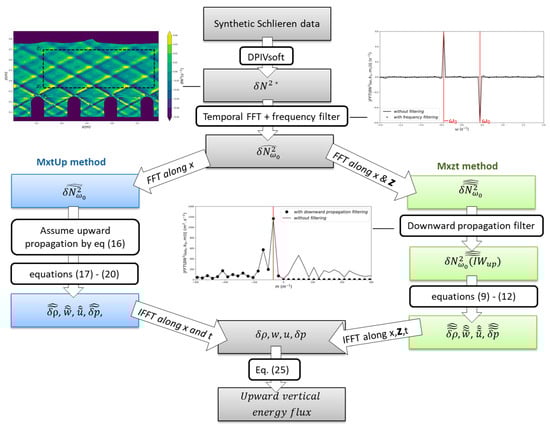
Figure 1.
Schematic chart of the Mxzt and MxtUp methods for calculating the density anomaly and the upward vertical energy flux from synthetic Schlieren data. * When applied to internal wave fields observed in the laboratory experiments (Section 3.2), a moving mean is applied along the z axis to the experimental data () in order to reduce the small-scale noise.
3. Results
To test our approaches, we will apply them to the data of for both analytical and experimentally measured internal wave fields. The analytical applications are described in Section 3.1, whilst the laboratory experiments and synthetic Schlieren measurements used are described in Section 3.2.
3.1. Evaluation of the Methods on Analytic Fields
The purpose of this section is to test and compare both methods on simple analytical fields (presented in the Section 3.1.1). To evaluate them, we quantify the error introduced on the resulting fields (Section 3.1.2) and on the vertical energy flux (Section 3.1.3).
3.1.1. Analytic IW Fields
• Ideal IW field
In a first test, we apply both methods to a linear and monochromatic IW field (referred to as IWideal), periodic in time (t) and space (x, z) and containing only waves with upward group velocity, i.e., downward phase velocity:
where the vertical wave number is given by:
where A is the amplitude, is the horizontal wavenumber, and corresponds to the angular frequency. By choosing the positive sign above, we ensure that the vertical phase velocity is negative, i.e., that the group velocity is positive and the energy flux upward.
• Damped IW field
In a second test, we apply our methods to a more realistic IW field (referred to as IWdamped), closer to experimental observations. The amplitude of the internal waves in laboratory experiments decreases upwards, away from the generation source. To represent this vertical damping analytically, we multiply the Brunt–Väisälä frequency anomaly in (26) by a decreasing exponential
where a is the vertical damping coefficient. The IWdamped field is therefore not periodic in z, in contrast to the IWideal field.
• Mixed IW field
The purpose of the final test is to test the strong hypothesis of upward energy propagation made in MxtUp. To this end, we add to the IWideal field in (26) an IW field containing only waves with downward group velocity (referred to as IWdown):
where B is the amplitude of the downward propagating waves. We choose B = 0.2 A.
In each case, internal waves propagate in a two-dimensional domain with and and in a time interval of . The size of this two-dimensional domain is selected to resemble the laboratory experiment of Section 3.2. This domain contains an integer number of wavelengths (two vertical wavelengths: m−1, ; three horizontal wavelengths: ; 10 time periods: as in the experiment of Section 3.2). The density stratification is linear, so that the Brunt–Väisälä frequency N is constant (N = 0.85 s−1) and larger than the angular frequency of the internal wave. The amplitude A is set to 0.02 s−2, and the vertical damping coefficient a is set to 0.62 . The vertical damping coefficient a is chosen to correspond to the mean vertical decrease observed in the experiment (τ = −20%, see below in Section 3.2.2).
The analytical density perturbation field corresponding to the Brunt–Väisälä frequency anomaly given by (26), (28) and (29) is obtained from (7) by integration along z:
3.1.2. Validation and Comparison of Reconstructed Fields
We will hereby test the two methods described in Section 2 on the analytic fields given by (26), (28) and (29). By applying (12) or (17) on these fields, we obtain the corresponding density perturbation fields numerically. They are then compared to the exact fields given by (30). We also differentiate the numerical fields along z to reconstruct the Brunt–Väisälä frequency anomaly using (7). The differentiation is performed using second order centred differences. The result is then compared to the original analytic fields . This comparison can also be executed for the laboratory experiment, where we have access to observational data for but not for .
To quantify the errors introduced by our methods, we calculate the normalized root mean squared (nrms) difference between the numerically reconstructed field () and the analytical field ()
where is either or .
The first step in determining from with the method Mxzt is to calculate the Fourier transform by FFT. Particular slices (for given values of and ) of the resulting 3D spectra for the three analytic fields are compared in Figure 2. The spectrum of (plain lines) is zero everywhere except at the fundamental vertical wavenumber . The spectral amplitude of (dashed lines) is slightly smaller at than that of , and the imaginary part of also shows peaks at and . These “artificial” harmonics in the spectrum of are caused by the non-periodicity of the IWdamped signal. The non-periodic signal is seen as a periodic discontinuous signal by the FFT, and the discontinuity distorts the spectrum by adding false overtones that are aliased into the spectrum. The figure also shows the spectrum of (dashed-dotted lines with circle markers). The real part has an additional peak at , which is the signature of the downward propagating beam (IWdown).
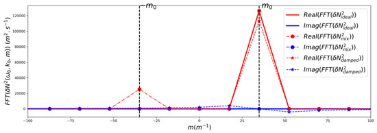
Figure 2.
Spectra of (solid lines), (dashed lines with star markers) and (dashed-dotted lines with circle markers) as a function of for and . Blue lines: imaginary part; red lines: real part.
• Ideal IW field
For the ideal IW field (IWideal), the nrms difference between δρ from the Mxzt method and the analytical δρ is . With the MxtUp method, the nrms difference for δρ is . As expected, therefore, in the ideal case, both methods give very small errors. The nrms difference between the reconstructed δN2 and the analytical δN2 is the same for both methods: . This error comes from differentiating along z by finite differences when using (7) to calculate δN2. The same error is obtained when differentiating numerically and comparing to .
• Damped IW field
For IWdamped, with the Mxzt method is , whereas with the MxtUp method is less than 2%. As expected, therefore, the non-periodicity of the signal degrades the accuracy of the Mxzt method. The MxtUp method, which doesn’t rely on the z-periodicity hypothesis, is the most accurate in this case. However, the MxtUp method still gives a larger error than in the ideal case ( instead of ). The larger the coefficient , the larger is the error of the resulting density field. For example, for a coefficient a of 1.7 , the error of the resulting density field is increased to 4.8%. One reason for this error may be that the ideal polarization relations for an inviscid fluid are used to reconstruct the density field. It would be possible, but more complicated, to use instead the viscous polarization relations, both when constructing the analytical solution and when reconstructing the density field. However, it is not clear that the damping in the experiment is in fact mainly caused by viscosity, and this error is in any case small compared to other error sources in the experiment.
Figure 3a compares the vertical profile of the rms error of the density anomaly field obtained with the Mxzt and MxtUp methods, averaged over and . With Mxzt, the largest errors occur at the upper and lower vertical boundaries. These errors are linked to Gibb’s oscillations. The FFT along z introduces artificial values of m (Figure 2), which result in an overestimate of the IW amplitude near the boundaries. With MxtUp, the errors increase with depth, as does the amplitude of the density anomaly field. This is because the error is not normalized by the local amplitude.
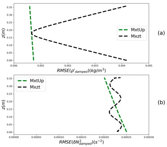
Figure 3.
Vertical profiles of the root mean square (rms) error, averaged over and , of the reconstructed fields for IWdamped resulting from the Mxzt and MxtUp methods. (a) rms error of . (b) rms error of .
The reconstructed field is obtained from the vertical derivative of the reconstructed field , using Equation (7). The normalized rms differences over the entire domain between the original and the reconstructed from the Mxzt and MxtUp methods are both 1.8%. Thus, for the Mxzt method, the error of the reconstructed field () is smaller than that of the reconstructed field (. Figure 3b compares the vertical profiles of the rms error of averaged over and for both Mxzt and MxtUp. For Mxzt (dashed black line), the rmse vertical profile presents several oscillations related to Gibb’s oscillation phenomenon.
• Mixed IW field
In the test case with the mixed wave field, our aim is to reconstruct only the upward wave component. We therefore calculate the nrms difference between the reconstructed fields of upward propagating waves and the IWideal analytical fields (not IWmix). The reference density anomaly field is thus . When using the Mxzt method, therefore, we first filter away (in Fourier space) all downward propagating wave components (with upward phase velocity) from the IWmix field () = 0), in order to reconstruct only the upward propagating wave’s field. The same filtering will be done below, when calculating the vertical energy flux from the experimental data in Section 3.2.2. This filter cannot be applied when using the MxtUp method, since it does not involve Fourier transformation in z.
For IWmix, with the Mxzt method is , wheras with the MxtUp method, is around 20%. Thus, as expected, the presence of downward propagating waves in the original signal degrades the accuracy of the MxtUp method. The error in the density field obtained with MxtUp is of the same magnitude as B/A (20%), the ratio of the amplitude of the downward propagating waves to the amplitude of the upward propagating waves. The Mxzt method is thus the most accurate in this case.
Figure 4a compares the vertical profile of the rms error of the reconstructed density anomaly field obtained with the Mxzt and MxtUp methods, averaged over and . With both methods, the error is homogeneous in depth.
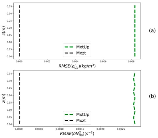
Figure 4.
Vertical profiles of the rms error, averaged over and , of the reconstructed upward propagating wave fields of IWmix resulting from the Mxzt and MxtUp methods. (a) rms error of . (b) rms error of .
The normalized rms difference over the entire domain between and the reconstructed from the Mxzt method is . This is the same as the error when calculating the vertical derivative. The value of with the MxtUp method (with as reference field) is around 20% (the same magnitude as B/A). Taking , the original signal, as reference field, the value of rises to above 39%.
Figure 4b compares the vertical profiles of the rms error of averaged over and for both Mxzt and MxtUp. For MxtUp (dashed green line), the rmse vertical profile presents several oscillations (four periods of oscillation). The downward propagating waves therefore induce artificial oscillations of the resulting field. The number of oscillations is proportional to the number of vertical wavelengths inside the domain ().
If we include x-variability in IWdown, for example, by multiplying it by a cosine function of x, the error induced by MxtUp on the reconstructed fields is no longer homogeneous along x. The rmse of the and fields are maximal where the amplitude of the downward propagating waves is maximal. This change has no impact on the resulting Mxzt fields, as the downward propagation is filtered away, and with it the heterogeneity along x.
On the other hand, if we include z-variability in IWdown, for example, by multiplying it by (a vertical damping similar to IWdamped but in the opposite direction), boundary errors appear on the resulting Mxzt field. The associated nrmse is therefore slightly increased: 0.4% and 0.6% for a = 0.62 .
3.1.3. Vertical Energy Flux
We hereby compare the vertical energy flux obtained from the reconstructed velocity and pressure fields with the analytical value. For the ideal IW field, we can obtain a simple analytical expression of the vertical energy flux from Equation (25):
where nx is the number of periods in the x-interval. The numerical energy flux is calculated by using the reconstructed fields w and in (25). The reconstructed fields w and are obtained from either (13) or (15) (for the Mxzt method), or (18) and (20) (for the MxtUp method).
Figure 5a shows the energy flux for the ideal IW field (IWideal, plain curves) and the damped IW field (IWdamped, dashed curves). The value given by (32) is shown by the red line. For IWideal, the nrms difference between the analytical value and the energy flux from both the Mxzt and MxtUp method is . This is of the same magnitude as the error caused by numerical differentiation. The results from both methods agree: the green and black plain lines are indistinguishable on Figure 5a, and the nrms difference between the energy flux from Mxzt and MxtUp is less than .
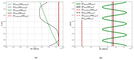
Figure 5.
(a) The vertical energy flux for IWdamped (dashed curves) and IWideal (plain curves) resulting from the MxtUp (green curves) and Mxzt (black curves) methods. The red curve represents the analytic vertical energy flux for IWideal, as defined by Equation (32). (b) Vertical energy flux for IWmix, obtained with MxtUp (green curve) and Mxzt (black curves); analytic flux in red, as defined by Equation (32). Plain curves are upward and dashed curves are downward flux. The black dotted line shows the total flux (upward minus downward) obtained with Mxzt and the combined field IWmix.
For IWdamped, the profiles of the vertical energy flux are very different with the two methods. With Mxzt (dashed black curve) the profile presents Gibb’s oscillations related to the non-periodicity of the IW field in z. The assumption that the fields are periodic in z forces the energy flux to be periodic, which means that it is overestimated at the upper boundary and underestimated at the lower boundary. The method MxtUp, on the other hand, accurately captures the vertical damping of the radiated energy away from the generation source.
Figure 5b shows the energy flux obtained from the mixed field IWmix. The analytic value obtained from (32) is shown separately for the upward and downward components (red lines). The values obtained with Mxzt are shown by the black lines. The nrms difference between the analytical value of the upward energy flux and the upward energy flux from the Mxzt method (plain black line) is . The Mxzt method also gives a very accurate solution for the downward energy flux (dashed black line), the nrms difference to the analytical value being only . The dotted line shows the flux obtained with the Mxzt method if the modes with (downward group velocity) are not filtered away from the Fourier spectrum of the mixed field. It is equal to the difference between the solutions for the upward and downward energy flux.
With MxtUp (green solid line), the profile has artificial oscillations linked to the existence of downward propagating waves in IWmix. The number of oscillations is proportional to the number of vertical wavelengths inside the domain. The nrms difference between the analytical profile of the upward vertical energy flux (red plain line) and the upward energy flux from the MxtUp method is 28%, which is in the same range as B/A (20%). Averaging over z, and comparing the mean of the MxtUp EF to the analytical value of the upward EF, the nrmse falls to 3.73%. This average overestimate is in the same range as the ratio of the downward flux EF to the upward EF: .
If we include x-variability in IWdown, for example, by multiplying it by a cosine function, IWdown is no longer perfectly periodic along x. Thus, the FFT along x introduces artificial harmonics of k, which affect the MxtUp method. The most significant impact is a slightly larger overestimation of the MxtUp EF average. This change has no impact on the Mxzt energy flux, as the downward propagating component is filtered away.
On the contrary, if we add z-variability to IWdown, for example, by multiplying it by (a vertical damping similar to IWdamped but in the opposite direction), Gibb’s oscillations appear in the Mxzt EF (both upward and downward). The nrmse on the upward EF profile is thus slightly increased: for a = 0.62 . However, the mean of the upward EF stays very close to the analytical value: 0.28% for 0.62 .
To conclude, for the ideal internal wave field (IWideal), both methods are very accurate and the errors of the reconstructed fields are close to zero. For the damped wave field (IWdamped), the signal is not periodic in z, and the periodic extension of the input signal is discontinuous at the upper and lower boundaries. Thus, the FFT along z introduces artificial higher harmonics of m (Figure 2). The false overtones corrupt the Mxzt method, creating Gibb’s oscillations. These oscillations result in errors near the upper and lower boundaries, both for the fields (Figure 3) and for the energy flux (Figure 5). Nevertheless, for a weak vertical damping, the errors stay in an acceptable range. The false overtones also slightly affect the MxtUp method by creating artificial modes with upward phase velocity. However, the induced errors in the calculated energy flux are very small even for a large vertical damping coefficient. The MxtUp method is therefore the most accurate one for the damped field.
On the other hand, since the MxtUp method rests on an upward propagation hypothesis, this method is not the most appropriate when the original wave field includes downward propagating waves. The downward propagating waves induce artificial oscillations in both the resulting field and the vertical energy flux. In addition, in this case, MxtUp overestimates the upward energy flux by slightly less than the ratio of the downward EF to the upward EF. For such a field, therefore, the Mxzt method is the most accurate one.
Both methods therefore have different strengths and weaknesses, closely related to the nature of the IW field investigated. In some cases, they can be complementary.
3.2. Application to Experimental Data
The intended application of these methods is for synthetic Schlieren obtained in water tank experiments. Thus, having verified the methods in the previous section, we now test them on experimental data (Section 3.2). In the tank-based experiment used, synthetic Schlieren measurements are made to obtain the Brunt–Väisälä frequency anomaly field.
3.2.1. Presentation of the Laboratory Experiments
To test our methods, data from experiments carried out in the large stratified water flume at the geophysical fluid dynamics laboratory of CNRM in Toulouse (France) are used. Built in 1982, this flume was initially designed for applied studies of atmospheric flows over complex terrain. It soon became used for research purposes, in particular for studies [16,17,18,19] on internal waves and boundary layers. The present experiments were designed to study internal waves generated over multiple ridges. Different topographic shapes and a large range of parameters have been studied. Here one selected case using a periodic topography composed of 10 ridges will be used.
The experiments were conducted in the flume used as a 22-m-long, 3-m-wide, and 1-m-high closed glass tank. A glass wall divided the tank into two parts, respectively 0.5 m and 2.5 m wide (Figure 6). The ridges were towed in the narrow part of the tank, while the wide part was used to dampen waves propagating horizontally from the two ends of the narrow part. Those waves were reflected into the wider part of the tank by deflectors covered with wave-damping material. The waves were then attenuated along sloping plates also covered with wave-damping material.
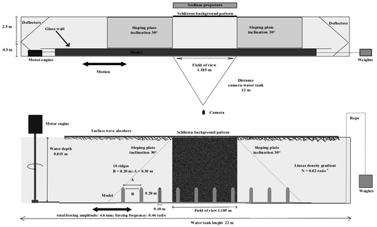
Figure 6.
Sketch of the experimental set-up. The top panel shows a view from the top whereas the bottom panel shows a view from the side. The rope and weights are used to create a symmetry in the forces moving the plate in both directions and improving the quality of the forcing. The horizontal to vertical ratio is not maintained for the sloping plates on the bottom panel.
The stratification was controlled by the salinity, while the laboratory air and water temperature were regulated at 20 °C. Two reservoirs filled with freshwater and brine, respectively, were connected to pumps that supply the tank with water. The mixture of freshwater and brine was then diffused through floating diffusers on the free surface. A computer controlled the flow of each pump to obtain a linear stratification over a depth of H = 81.5 cm. The background density profile was measured before and after each run in the fluid at rest using a carefully calibrated conductivity probe. A second similar density probe is placed in the tank at a fixed position in order to validate the density field reconstruction.
The topography is composed of 10 ridges with vertical side walls and rounded tops in order to mimic experimentally a periodic array of thin vertical walls as in the theoretical study of Nycander [8]. The distance between adjacent ridges is 20 cm, the width of each ridge is l = 10 cm, and the total height of the ridge is h0 = 20 cm (15 cm for the vertical part plus 5 cm for the half-circle with a radius of 5 cm covering the top). This periodic topography is attached to a long plate, in turn linked to a motor, forcing a sinusoidal back and forth motion at a precisely controlled frequency and amplitude. After the initial density profile has been established and measured, therefore, the topographic obstacle is moved at a given tidal frequency. This allows a better control of the forcing amplitude and frequency than in a set up with a fluid being pushed back and forth, as in the ocean. The equivalence between forcing by the barotropic tide and the oscillating topography for the generation of internal gravity waves has been shown by Gerkema and Zimmerman [20] in the linear case.
In the experiment used here, the amplitude of the forcing is 4.6 mm (defined as the distance between the extreme positions), the forcing frequency is 0.44 rad/s and the Brunt–Väisälä frequency of the background density profile is N = 0.82 rad/s. Wave absorbers are used at the top with a thickness of about 10 cm in order to avoid waves reflected at the upper surface, and thereby mimic an infinitely deep ocean as in the theoretical study of Nycander [8]. The wave absorbers at the top are made of the same wave-damping material that covers the deflectors and sloping plates mentioned above.
The laboratory system for determining the Brunt–Väisälä frequency anomaly field by the synthetic Schlieren method is shown in Figure 6. The measurements are performed using a PCO2000 CCD camera of the brand PCO, placed 12 m from the tank. Sodium lamps are placed behind a background pattern. The camera images a 1.185 m-wide region extending along 4 of the 10 ridges. Images are taken at a frequency of 20 images per period of ridge oscillation.
The processing is performed as follows. First of all the apparent distortion of the background pattern, due to the bending of optical rays related to wave induced local density changes in the tank, is captured by the camera. This apparent displacement relative to the image captured by the camera when there are no waves in the tank (fluid at rest) is quantified on a regular grid with a horizontal and vertical step of 2.2 mm using the PIV software DPIVsoft (described in detail by Meunier and Leweke [21] and Meunier et al. [22]). This displacement is then converted to the corresponding Brunt–Väisälä frequency anomaly on the same grid. The linear relation between the vertical apparent displacement and the index of refraction of the density-stratified fluid is given in detail by Dossmann et al. [23].
3.2.2. Application to Experimental Data
We apply both methods for calculating the wave fields and the energy flux to an experiment with forcing frequency ω = 0.44 rad/s (T = 14.2 s). Figure 7a shows the basic experimental data, the Brunt–Väisälä frequency anomaly field obtained from synthetic Schlieren measurements at t = 24 T. In this experiment, the downward propagating IW beams generated at the ridge tops are first reflected on the neighbouring ridge and then on the tank bottom, midway between two ridges, and finally on the original ridge, as illustrated in Figure 8. This leads to a constructive interference between the IW beams. The experiment is thus characterized by an intense generation of internal waves due to a resonance phenomenon with the periodic topography.
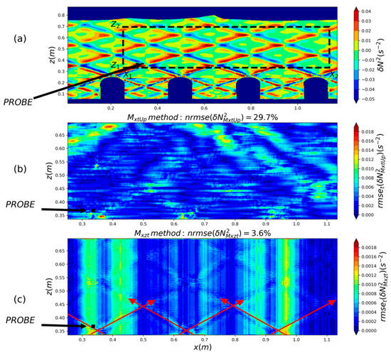
Figure 7.
Application of the two methods to experimental data. (a) Brunt–Väisälä frequency anomaly obtained from synthetic Schlieren measurements at t = 24 T. The black square represents the conductivity probe position. The dashed line locates the finite-space window () selected for the Mxzt & MxtUp methods, and used in the lower panels. (b) Root mean square error of the reconstructed field. To calculate the rmse, the field filtered at the fundamental frequency (denoted ) is used as the reference field. (c) Root mean square error of the reconstructed field (with reference field ). The red arrows represent the path of the primary beams.
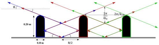
Figure 8.
Sketch of the experimental arrangement in the second resonance condition (. The arrows represent the path of the primary beams. The downward propagating IW beams are first reflected on the neighbouring wall and then on the tank bottom, midway between two rounded ridges, and finally on the original ridge. The phase is constant along each beam, and changes by at each reflection on a solid surface. This leads to a constructive interference between the IW beams: the downward propagating IW beam generated by the blue ridge (blue arrow) is superimposed on the upward propagating IW beam generated by the red ridge (red arrow).
The forcing frequency determines the IW beam angle, , and thus influences the reflection point on the neighboring obstacle and on the ground. Hence, the interference between the IW beams is determined by the forcing frequency ω and by the distance B between two ridges. Several IW beam angles can lead to constructive interference, depending on the number of reflections of the IW beams. For the first resonance, there is only one reflection, on the ground, and the downward propagating beam is inclined 58.7° to the horizontal. For the second resonance (illustrated in Figure 8), there are three reflections, two at ridges and one on the ground, and the downward propagating beam is inclined 30.7° to the horizontal. For some forcing frequency between the first two resonances, the downward propagating IWs beams are reflected in the corner between the ridge and the ground. In this case, the interference between the beams is destructive and the energy is trapped between the ridges.
The IW beam angle observed on the Schlieren data in Figure 7a is 32°. This is quite close to the theoretical beam angle calculated from the forcing frequency and the Brunt–Väisälä frequency of the experiment ().
• Selection of a finite-extent window
To apply the Mxzt & MxtUp methods to the experimental data, we need to define a finite space-time window with an integer number of periods along t, x and z. Otherwise, artificial harmonics appear in the FFT spectrum. To optimize the x- and z-intervals, we calculated the rms difference between the signals at the boundaries of the finite-space window (the dashed lines in Figure 7a). If the field is perfectly periodic and if the finite-space window contains an integer number of periods, then the signals at opposite boundaries of the finite-space window are identical. Hence, the x- and z-boundaries are chosen to minimize the rms difference.
Selecting a finite-time interval is easier, since we know exactly the initialization time and the forcing period (determined by the motor frequency). The experiments are conducted during 30 periods. We select the last ten periods, which is well after any noticeable transient effects. To reduce the small-scale noise, a moving mean with a short window of five points along the z axis is applied to the experimental data. Since harmonics can be generated by the ridges and by nonlinear processes, the experimental data inside the finite-extent window, , are filtered in frequency space, keeping only the component with frequency . The Mxzt and MxtUp methods are then applied to this filtered field, denoted .
• Validation and density field reconstruction
Given the filtered Brunt–Väisälä frequency anomaly fields obtained from the synthetic Schlieren measurements, we calculate the instantaneous density anomaly, vertical velocity and pressure either from (12), (13) and (15), for the Mxzt method, or from (17), (18) and (20), for the MxtUp method. The energy flux is then calculated from (25), and the reconstructed field from (7). It was not possible to measure the density anomaly field everywhere in the experiments, but one conductivity probe measured it locally (black square on Figure 7).
To quantify the errors introduced by both methods, we calculate the rms difference between the reconstructed Brunt–Väisälä frequency anomaly fields ( and ) and the corresponding fields obtained from the synthetic Schlieren measurements (). As in the analytic examples, the reconstructed Brunt–Väisälä frequency anomaly fields are obtained by numerical differentiation of the instantaneous density anomalies ( and ) using (7). Figure 7 shows the spatial distribution of the errors introduced by the MxtUp method in Figure 7b, and by the Mxzt method in Figure 7c.
For both methods, the errors are larger near the beams. This is expected, since the rms errors are not normalized by the local amplitude. Judging from the analytic examples, we should use the MxtUp method, since in the experimental data, the periodicity is much better along x than along z. However, the global and normalized rms difference between and is more than , wheras it is only 3.6% between and . Mxzt therefore seems to be the most accurate method. To understand this result, we take a closer look at the differences between the MxtUp and Mxzt reconstructed Brunt–Väisälä frequency anomaly fields.
It can be seen from Figure 7 that although the vertical variations of the reference field were smoothed, the small-scale noise is much stronger with the MxtUp method than with the Mxzt method. One reason for that is that the calculation of the density anomaly field is made independently for each value of z in the MxtUp method. In contrast, in Mxzt, the Fourier transformation along z effectively acts as a filter (less small-scale noise on Figure 7c).
The Mxzt method slightly underestimates the anomalies at the lower vertical boundaries, inducing the largest errors at the bottom of the finite-space window (Figure 7c). In the analytic examples, the largest errors at the vertical boundary are induced indirectly by the vertical damping of the IW field. Such damping corrupts the periodicity of the signal along z and induces Gibbs oscillation (Section 3.1.2). To quantify the vertical damping of the IW field, the decrease factor is calculated. At each time step, , a damping coefficient is first determined by fitting (averaged over x) to the form , where A is the amplitude of the Brunt–Väisälä frequency anomaly. We obtained a mean decrease of −20% defined from the damping coefficient and the domain vertical length ΔZ as . Using such a damping coefficient in the formula of the ideal IW field (Section 3.1.1 Equation (28)) gives an estimation of the error in the field of 2%, which is reasonably small.
The experimental IW field has another important feature. There are visible peaks in the m-k spectrum corresponding to wave components with upward phase velocity (downward energy flux). These could be caused by partial reflection at the upper boundary, as wave absorbers used at the top may not completely suppress the reflected waves. They could also be generated inside the water volume by nonlinear interactions. These wave components are treated incorrectly by the assumption of upward energy propagation made in MxtUp. In Figure 7b, supplementary patterns appear in both of the upper corners of the finite-space window, resembling downward propagating beams. Hence, in this experiment, upward propagating beams are indeed partially reflected, inducing the propagation of downward IW beams. The MxtUp method assumes that these downward propagating IWs don’t exist, which is a source of errors (as shown in Section 3.1.2).
To perform a local validation of our methods, density measurements are performed at a fixed position inside the IW beam with a conductivity probe. A local averaging of the density anomaly or , which was obtained from Mxzt or MxtUp, is performed over a square of side 1.1 cm around the conductivity probe location (corresponding roughly to the measurement volume of the conductivity probe). The comparison between the time series is shown in Figure 9. As our “spectral” methods are applied to synthetic Schlieren measurements filtered at the forcing frequency, the measurements of the conductivity probe are also filtered at the forcing frequency (black dashed curve). The amplitudes of these curves are very similar and the lag between them is not significant. Both methods (blue and green curves) induce a relative bias compared to the filtered conductivity measurement of 0.4% and a standard deviation of less than 18%. Both methods are therefore able to reconstruct the actual density field from synthetic Schlieren data.
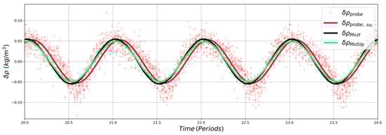
Figure 9.
Density measurement filtered at the fundamental frequency ω0 (red curve) and estimation (black and green curves) of the density anomaly from synthetic Schlieren using our two methods. Measurements are taken at a location (black square on Figure 7) in the middle of an upward propagating ray. The red crosses represent the raw probe data.
• Vertical energy fluxes
Given the reconstructed velocity and pressure fields, we obtain by numerical integration the vertical energy flux (cf Section 2.3) using both methods (EFMxzt & EFMxtUp). When using the Mxzt method, we first filter away all downward propagating wave components (with upward phase velocity) from the experimental data, as illustrated in Figure 10. This filtering cannot be done with the MxtUp method. This filtering was also not performed when calculating the error of the reconstructed in Figure 7, and when comparing the calculated to the probe measurements in Figure 9. The resulting profiles of the energy flux are shown in Figure 11.
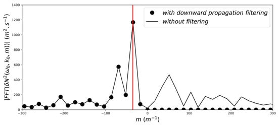
Figure 10.
Spectrum of as a function of for and . The plain line represents the spectrum of the raw data () whereas the dotted line represents the spectrum of the filtered data (without the downward propagation). The red vertical line indicates the value of m0.
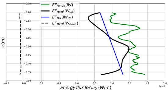
Figure 11.
Upward (plain curves) and downward (dashed curve, only for the Mxzt method) energy flux resulting from the MxtUp (green curve) and Mxzt (black curve) methods, associated with the fundamental frequency ω0. The blue line represents a mixed solution for the upward energy flux constructed from the mean slope of the MxtUp solution and the mean of the Mxzt solution.
The Mxzt upward energy flux (black plain line) contains Gibb’s oscillations related to the non-periodicity of the IWs field in z. In particular, one can see that the Mxzt method forces the computed energy flux to be the same at the upper and lower boundaries, which clearly is not the case in reality. As in the analytic examples, the number of oscillations is proportional to the number of vertical wavelengths inside the finite-space windows.
The MxtUp EF profile (green line) exhibits larger artificial oscillations, particularly in the upper part of the profile. These oscillations are related to the underlying assumption of upward energy propagation. Indeed, in this experiment, the upward propagating beams are partially reflected, inducing the propagation of downward IW beams. These downward propagating IWs induce errors when using MxtUp with the experimental data. And the mean of MxtUp EF is 16% larger than the mean of Mxzt EF. This overestimate of the upward EF using MxtUp is also related to the existence of downward propagating IWs (cf. Section 3.1.3). Nevertheless, the nrms difference between the upward energy flux obtained with the two methods is less than 2. Both profiles also tend to decrease vertically. This is consistent with the vertical damping of the wave field away from the generation source. The trend of the MxtUp EF profile should be the most accurate one, as the Mxzt EF trend is corrupted by the Gibb’s oscillations.
A mixed solution for the upward EF is proposed in Figure 11 (blue line). This mixed solution takes advantage of both methods. The slope of this solution is calculated from the MxtUp EF profile with a linear least squares fitting method whereas the mean is calculated from the Mxzt EF profile.
The Mxzt downward EF (black dashed line) also presents Gibb’s oscillations related to the non-periodicity of the IW field in z. The ratio of the downward flux to the upward flux is around 4%.
We finally compare the measured vertical energy flux to the theory of Nycander [8] and the numerical simulations by Zhang and Swinney [24]. According to Equation (9) in Nycander [8], the energy conversion by a periodic array of thin walls per meter along one of the walls is given by
where
Here, is the distance between the walls, the maximum velocity of the barotropic tide, and the nondimensional ridge height (or slope parameter). The conversion by an isolated ridge is obtained in the limit . In this limit, , which gives
The expressions have here been corrected for non-hydrostatic effects by replacing by .
We use the following parameters from our experiment: ω = 0.44 s−1, N = 0.82 s−1, H = 0.2 m, L = 0.2 m and , where the tidal amplitude is 2.3 mm. With these values, we obtain k = 0.29 × 10⁻⁶ W/m and Ciso = 22.3 × 10⁻⁶ W/m. The energy flux measured in our experiment is approximately 1 × 10⁻⁶ W/m per ridge, as seen in Figure 11. It is difficult to compare this to the theoretical value given by Equation (33), since the geometric factor is singular at the resonances, and therefore very sensitive to the exact value of S near a resonance. Furthermore, the theoretical value is certainly not singular when there is a finite number of ridges rather than a periodic array, and the ridges in the experiment are rather broad and have rounded tops. Nevertheless, it is interesting to note that the measured energy flux is slightly more than three times larger than the dimensional factor k in Equation (33).
According to Figure 1 in Zhang and Swinney (2014), the simulated energy conversion at the second resonance is around 10% of the theoretical conversion by a single ridge of the same height, while the energy flux in our experiment is around 5% of the value for a single ridge. Again, we cannot expect a close agreement with the numerical simulations, since the energy conversion is sensitive to the exact value of the ridge height close to resonance, and since the ridges were much thinner in the numerical simulations than in our experiment. Considering this, we believe that there is a satisfactory agreement between the energy fluxes from our experiment and the numerical simulations of Zhang and Swinney (2014).
4. Discussion and Conclusions
We have presented two different spectral methods for calculating the density and the vertical energy flux from synthetic Schlieren measurement data (fields of ), valid for a periodic field of linear internal waves in a density-stratified fluid with a uniform buoyancy frequency N. With both methods, the various fields are obtained from by Fourier transformation (using FFT) and assuming linear relations. Then, the energy flux is obtained as the product of the fields and w. The two approaches operate under different assumptions, and the choice between them depends on the situation. The Mxzt method rests on the assumption of a periodic IW field in the three dimensions (x, z, t), whereas the MxtUp method assumes that the IW field is periodic in x and t and composed solely of wave components with downward phase velocity (i.e., upward group velocity and energy flux).
Both methods were verified using analytic fields , and then applied to synthetic Schlieren data obtained from a water tank experiment. The experiment was designed to study internal waves generated over multiple ridges. In this experiment, internal waves are generated by a periodic topography composed of 10 ridges. The basic assumptions of x- and t- periodicity are therefore well satisfied. However, the z-periodicity assumption of Mxzt is not strictly valid since the internal wave amplitude decreases weakly upwards, mainly because of viscosity. The assumption of upward propagation is also not fully satisfied in the experiment, as some residual reflections from the wave absorbers at the upper boundary still exist.
The two methods succeed in reconstructing the density anomaly field. The reconstructed from the Schlieren data with the Mxzt method agrees within 4% with the Schlieren data. The errors in therefore remain in a very acceptable range. With the MxtUp method, the calculation of the density anomaly, velocity, pressure, and energy flux is made independently for each value of z, which results in small-scale noise. This small-scale noise is partly responsible for a larger error in the resulting .
In the experiment, there is a weak vertical decrease in the internal wave amplitude (τ ≈ −20%). The effect of this upward-decreasing amplitude was tested analytically by adding a vertical damping to the ideal IW field. In that case, the FFT along z introduces artificial higher harmonics of the vertical wavenumber m, which corrupt the Mxzt method by creating Gibb’s oscillations. These oscillations result in errors near the upper and lower boundaries, both for the fields (ρ, p, w) and for the energy flux. Nevertheless, for a weak vertical damping, the errors of the fields stay in an acceptable range (2% for τ ≈ −20%, as in the experiment). The false overtones can also slightly affect the MxtUp method by creating artificial modes with upward phase velocity. However, the induced errors are very small even for large vertical damping (<5% for τ = −45%). Hence, the upward-decreasing amplitude is not a major issue for the two methods when applied to laboratory experiments.
A substantial part of the errors induced by the MxtUp method is linked to the assumption of upward propagation. As shown when the Mxzt method is applied, some reflected waves propagate downwards in the experiment. The effect of these residual reflections was tested analytically by adding downward propagating waves to the ideal IW field. As expected, the presence of downward propagating waves in the signal degrades the accuracy of the MxtUp method. It induces artificial oscillations in the fields () and in the energy flux. The average energy flux is also overestimated by an amount slightly smaller than the downward energy flux. This error doesn’t exist in the Mxzt method as it takes into account both propagation directions.
Hence, on the one hand, the Mxzt method induces artificial Gibb’s oscillations but can be used to estimate the mean upward energy flux. On the other hand, the MxtUp method overestimates the mean upward energy flux but can be used to estimate the average vertical profile of the upward energy flux. Consequently, a mixed solution is proposed for the upward energy flux using the benefits of both methods: the trend from the MxtUp energy flux and the mean from the Mxzt energy flux. However, the Mxzt method is the only method that can be used to calculate the downward part of the energy flux. This estimate cannot be done with MxtUp, which simply assumes that all flux is upward.
The methods presented in this paper could likely still be improved. For example, inspired by Hazewinkel et al. [25], one could use both the horizontal and the vertical components of the synthetic Schlieren apparent displacement, which may contribute to removing some small-scale noise. Another possibility for future improvement could be to include viscous damping in the polarization relations used to obtain the velocity and the pressure field.
Besides energy fluxes, the methods allow the computation of the density field from synthetic Schlieren data collected in laboratory experiments, which opens interesting perspectives for this type of data analysis. Future work will focus on determining the scaling of the energy flux with topographic height in the supercritical regime using the whole dataset from which the experiment used in this paper has been extracted. This is an important issue for the computation of energy flux from barotropic tides to internal waves in the global ocean. Resonance phenomena with periodic supercritical topography [8] will also be part of this future work. Another step could be to extend this work for laboratory experiments to three-dimensional topography with two possible approaches: (i) with synthetic Schlieren but looking at the experiment from different angles using multiple-cameras or a plenoptic camera (see for example [26]), (ii) from multi-planes 2D PIV or from 3D PIV.
Author Contributions
Conceptualization, J.N. and A.P.; Data curation, A.P.; Funding acquisition, J.N. and A.P.; Methodology, J.N.; Project administration, J.N. and A.P.; Supervision, J.N. and A.P.; Validation, L.B.; Writing—original draft preparation, L.B.; Writing—review and editing, J.N. and A.P. All authors have read and agreed to the published version of the manuscript.
Funding
The synthetic Schlieren data used in this study came from experiments supported by the European Union’s Seventh Framework Programme, through the grant to the budget of the Integrating Activity HYDRALAB IV, within the Transnational Access Activities, Contract No. 261520. The contribution of Lucie Bordois to this study was supported by CNRS, METEO-FRANCE and the University of Stockholm.
Acknowledgments
We thankfully acknowledge Anne Belleudy, Radiance Calmer, Jean-Christophe Canonici, Frédéric Murguet and Vivian Valette for their contribution to setting up and running the experiments, as well as Yong Sung Park and Saeed Falahat for their participation in these experiments. Figure 6 was inspired by an original sketch of Anne Belleudy and Radiance Calmer.
Conflicts of Interest
The authors declare no conflict of interest. The funders had no role in the design of the study; in the collection, analyses, or interpretation of data; in the writing of the manuscript, or in the decision to publish the results.
References
- Munk, W.; Wunsch, C. Abyssal recipes II: Energetics of tidal and wind mixing. Deep Sea Res. Part Oceanogr. Res. Pap. 1998, 45, 1977–2010. [Google Scholar] [CrossRef]
- Nycander, J. Generation of internal waves in the deep ocean by tides. J. Geophys. Res. Oceans 2005, 110. [Google Scholar] [CrossRef]
- Bell, T.H. Lee waves in stratified flows with simple harmonic time dependence. J. Fluid Mech. 1975, 67, 705–722. [Google Scholar] [CrossRef]
- Melet, A.; Nikurashin, M.; Muller, C.; Falahat, S.; Nycander, J.; Timko, P.G.; Arbic, B.K.; Goff, J.A. Internal tide generation by abyssal hills using analytical theory. J. Geophys. Res. Oceans 2013, 118, 6303–6318. [Google Scholar] [CrossRef]
- Smith, S.G.L.; Young, W.R. Tidal conversion at a very steep ridge. J. Fluid Mech. 2003, 495, 175–191. [Google Scholar] [CrossRef]
- Laurent, L.S.; Stringer, S.; Garrett, C.; Perrault-Joncas, D. The generation of internal tides at abrupt topography. Deep Sea Res. Part Oceanogr. Res. Pap. 2003, 50, 987–1003. [Google Scholar] [CrossRef]
- Pétrélis, F.; Smith, S.L.; Young, W.R. Tidal conversion at a submarine ridge. J. Phys. Oceanogr. 2006, 36, 1053–1071. [Google Scholar] [CrossRef]
- Nycander, J. Tidal generation of internal waves from a periodic array of steep ridges. J. Fluid Mech. 2006, 567, 415–432. [Google Scholar] [CrossRef]
- Balmforth, N.J.; Peacock, T. Tidal conversion by supercritical topography. J. Phys. Oceanogr. 2009, 39, 1965–1974. [Google Scholar] [CrossRef]
- Peacock, T.; Echeverri, P.; Balmforth, N.J. An Experimental investigation of internal tide generation by two-dimensional topography. J. Phys. Oceanogr. 2008, 38, 235–242. [Google Scholar] [CrossRef]
- Echeverri, P.; Flynn, M.R.; Winters, K.B.; Peacock, T. Low-mode internal tide generation by topography: An experimental and numerical investigation. J. Fluid Mech. 2009, 636, 91–108. [Google Scholar] [CrossRef]
- King, B.; Zhang, H.P.; Swinney, H.L. Tidal flow over three-dimensional topography in a stratified fluid. Phys. Fluids 2009, 21, 116601. [Google Scholar] [CrossRef]
- Allshouse, M.R.; Lee, F.M.; Morrison, P.J.; Swinney, H.L. Internal wave pressure, velocity, and energy flux from density perturbations. Phys. Rev. Fluids 2016, 1, 014301. [Google Scholar] [CrossRef]
- Clark, H.A.; Sutherland, B.R. Generation, propagation, and breaking of an internal wave beam. Phys. Fluids 2010, 22, 076601. [Google Scholar] [CrossRef]
- Sutherland, B.R.; Dalziel, S.B.; Hughes, G.O.; Linden, P.F. Visualization and measurement of internal waves by ‘synthetic schlieren’. Part 1. Vertically oscillating cylinder. J. Fluid Mech. 1999, 390, 93–126. [Google Scholar] [CrossRef]
- Knigge, C.; Etling, D.; Paci, A.; Eiff, O. Laboratory experiments on mountain-induced rotors. Q. J. R. Meteorol. Soc. 2010, 136, 442–450. [Google Scholar] [CrossRef]
- Lacaze, L.; Paci, A.; Cid, E.; Cazin, S.; Eiff, O.; Esler, J.G.; Johnson, E.R. Wave patterns generated by an axisymmetric obstacle in a two-layer flow. Exp. Fluids 2013, 54, 1618. [Google Scholar] [CrossRef][Green Version]
- Dossmann, Y.; Paci, A.; Auclair, F.; Lepilliez, M.; Cid, E. Topographically induced internal solitary waves in a pycnocline: Ultrasonic probes and stereo-correlation measurements. Phys. Fluids 1994 Present 2014, 26, 056601. [Google Scholar] [CrossRef]
- Stiperski, I.; Serafin, S.; Paci, A.; Ágústsson, H.; Belleudy, A.; Calmer, R.; Horvath, K.; Knigge, C.; Sachsperger, J.; Strauss, L.; et al. Water tank experiments on stratified flow over double mountain-shaped obstacles at high-reynolds number. Atmosphere 2017, 8, 13. [Google Scholar] [CrossRef]
- Gerkema, T.; Zimmerman, J.T.F. Generation of nonlinear internal tides and solitary waves. J. Phys. Oceanogr. 1995, 25, 1081–1094. [Google Scholar] [CrossRef]
- Meunier, P.; Leweke, T. Analysis and treatment of errors due to high velocity gradients in particle image velocimetry. Exp. Fluids 2003, 35, 408–421. [Google Scholar] [CrossRef]
- Meunier, P.; Leweke, T.; Lebescond, R.; van Aughem, B.; Wang, C. DPIVsoft User Guide; Institut de Recherches sur les Phénomènes Hors Equilibre, Universités Aix-Marseille I et II: Marseille, France, 2004. [Google Scholar]
- Dossmann, Y.; Paci, A.; Auclair, F.; Floor, J.W. Simultaneous velocity and density measurements for an energy-based approach to internal waves generated over a ridge. Exp. Fluids 2011, 51, 1013–1028. [Google Scholar] [CrossRef]
- Zhang, L.; Swinney, H.L. Virtual seafloor reduces internal wave generation by tidal flow. Phys. Rev. Lett. 2014, 112, 104502. [Google Scholar] [CrossRef] [PubMed]
- Hazewinkel, J.; Grisouard, N.; Dalziel, S. Comparison of laboratory and numerically observed scalar fields of an internal wave attractor. Eur. J. Mech. B Fluids 2011, 30, 51–56. [Google Scholar] [CrossRef]
- Bichal, A. Development of 3D Background Oriented Schlieren with a Plenoptic Camera. Ph.D. Thesis, Auburn University, Auburn, AL, USA, August 2015. Available online: http://hdl.handle.net/10415/4827 (accessed on 24 June 2020).


© 2020 by the authors. Licensee MDPI, Basel, Switzerland. This article is an open access article distributed under the terms and conditions of the Creative Commons Attribution (CC BY) license (http://creativecommons.org/licenses/by/4.0/).