Numerical Simulation of Breathing Mode Oscillation on Bubble Detachment

Abstract

When a bubble detaches from a nozzle immersed in water, a sound is emitted owing to the detachment. The bubble deformation and sound emission generated after detachment has been investigated in many studies, in which the breathing mode with a natural frequency was discussed based on the dynamics of the interface between the air and water. In this study, the deformation of a bubble was observed, and the sound emitted upon detachment was measured experimentally. To analyze the bubble deformation process, a computational fluid dynamics (CFD) simulation was conducted using the volume of fluid (VOF) method to predict the sound emission. In the analysis, the deformation behavior, the oscillation frequencies, sound pressure, and radius variation were discussed by comparing the numerical and experimental data. Furthermore, the natural frequency and low frequency vibrations were discussed based on the interference between the detached bubbles and the air column vibrations.

1. Introduction

An instant deformation of a bubble observed on bubble detachment or collision in water frequently accompanies sound emission. Such sound or noise has been a concern in many devices and equipment in engineering. For this two-phase flow problem, many studies have been conducted. Before discussing such engineering problems, we introduce a relevant, interesting, and simple traditional instrument used in the Japanese traditional culture “Suikinkutsu”. This Japanese word translates to “water pot harp” and produces a pleasant and favorable sound when droplets collide on the surface of water. In addition to the common musical instrument, Suikinkutsu consists of a sound generator and resonator. The resonator is constructed using chinaware, and the resonating sound is emitted through a bamboo duct. The sound generation system is significantly sophisticated to generate a favorite sound. Such a sound generation protocol was reported in previous studies [1,2], which may be influential and of interest to subjects in the field of fluid dynamics. Watanabe [1] reported that the sound was generated by the detachment of bubbles, which was introduced by the collision of a series of droplets attacking the water surface. Here, one should note that the musical instruments are constructed with a sound source with natural frequency and the resonator (water pot), which enhances the original sound. Our present research focuses on the sound source accompanied by bubble detachment.

Regarding engineering problems, we sometimes experience sound emission in a two-phase flow of air, water, or cavitation flow. Studies on the sound and vibrations of submerged air bubbles began with Rayleigh’s experiment on the collapse of cavitation bubbles [3] and Minnaert’s experiment on running water with air bubbles [4]. Rayleigh investigated the collapse time of a spherical vacuum cavity in water in terms of the energy conservation law. Afterward, that model was expanded to the general problem, in which the cavity was replaced with a gas bubble, as done in the Rayleigh model. The equation of motion derived in the Rayleigh model was developed using Rayleigh’s equation, considering the various effects of physical properties such as viscosity, compressibility, surface tension, evaporation, and condensation. The fundamental equation is currently known as the Rayleigh and Plesset equation [5]. Furthermore, Minnaert experimented by introducing air into the flowing water. The bubble detached from the nozzle into the water, vibrated continuously, and appeared to be a single resonance system such as a mass addition to the surrounding fluid. An air bubble that vibrates in water is often called the “Minnaert bubble.” The formula of the oscillatory frequency is called Minnaert’s equation, and it is still used for estimating the natural frequency of the radiated sound. In this analysis, the primary natural oscillation is called the breathing mode. Strasberg [6] and Longuet-Higgins [7,8,9] also conducted experimental and theoretical studies on bubble shapes and sound wave generation. Theoretical and experimental studies were conducted by Oguz [10] and the natural frequency of a gas bubble in a tube was also studied by the same authors [11]. A theoretical approach for the Minnaert bubble was developed by Leighton [12] and Devaud et al. [13]. In their studies, the acoustic signal propagation was analyzed for the pulsating air bubble under different boundary conditions, and a singular resonant motion was represented in detail.

Manasseh et al. [14] experimentally measured the sound generation on bubble coalescence. In addition, regarding the acoustic emission from the bubble, Czerski and Deane [15] studied the acoustic excitation of bubbles and tested a simple analytical model of the collapse of the bubble neck. They discussed the role of the surface tension by capturing the surface behavior with a high-speed video camera. They concluded that the neck collapse progressed due to the local dynamics, which depended on the surface tension and the shape of the neck but not on the rest of the bubble. Recently, the sound accompanying the dripped tap was measured experimentally [16]. This report discussed the oscillation of an entrapped air bubble. In addition, Bari and Robinson investigated the bubble shape and local pressure acting on the bubble interface and forces in an experimental study [17].

Annaland et al. [18], Quan and Hua [19], Hanafizadeh [20], Ambrose et al. [21], and Xi [22] conducted numerical studies to investigate the bubble deformation process by adopting the higher-order polynomial interface capturing scheme, and the volume of fluid (VOF) method. The VOF method is an interface-capturing technique and has the advantage of a simple algorithm and versatile applicability. These reports were successful in simulating the deformation process of rising bubbles in water. Furthermore, some papers discussed the deformation process with acoustic signal prediction. Bui and Manasseh [23] reported the pressure profiles obtained by experiment and simulation. The pressure waveform obtained by the simulation showed agreement within the same order as the experimental data during the first few cycles. However, the frequency of the simulation disagreed with the experimental data, which was three times higher than the experimental data. Liu et al. [24,25] performed a bubble deformation and acoustic characteristics simulation using a combination of the large eddy simulation (LES), VOF, and Ffowcs Williams–Hawkings (FW-H) methods. In their study, the hybrid method was successfully used to simulate the bubble deformation and calculate the acoustic signal. In addition, they concluded that the nozzle wall structure affected the bubble formation. Unfortunately, the acoustic pressure signal was too small, and we could not find a comparison between the experimental and numerical pressure signals.

In the present study, the sound pressure generated by single bubble detachment was a target reproduced by CFD. Using a finite volume differential scheme combined with the VOF method, the pressure profile and bubble radius variation were discussed. The pressure level was compared with the experimental result, and the temporal pressure field was demonstrated to discuss the acoustical resonance process.

2. Experiment

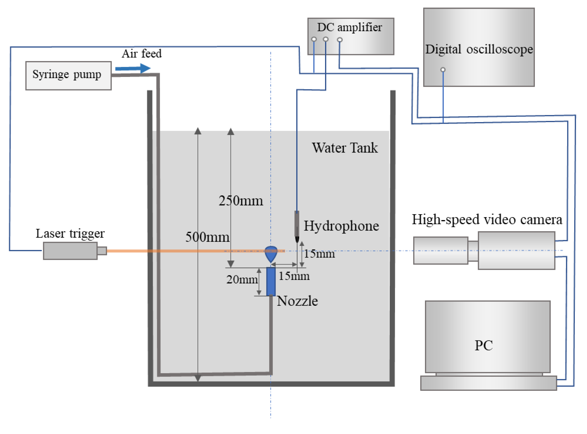
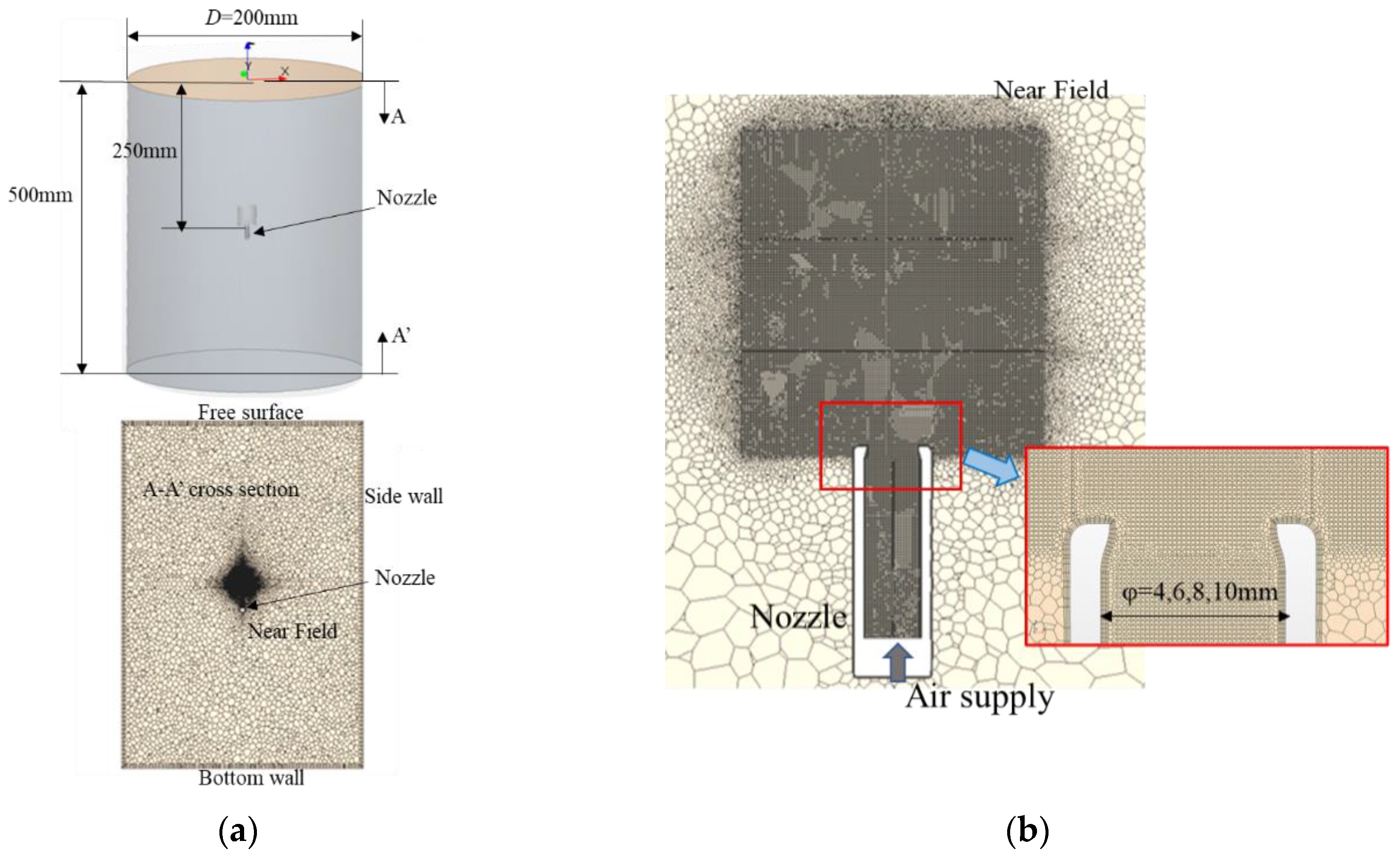
2.1. Experimental Apparatus

Figure 1 shows the experimental apparatus used in the present experiment. Air bubbles were generated from a nozzle immersed in water. The deformation of the bubble was visualized using a high-speed camera (IDT, XS5), and the sound emission was measured using a hydrophone (Bruel & Kjaer, type-8103, sensitivity 25.6 μV/Pa). The pressure signal, which was amplified using a charge amplifier (Bruel & Kjaer, type-2635), was transferred to a personal computer via an AD converter (NI, 6251). Because the natural frequency of the breathing mode accompanied by bubble release was approximately 1 kHz, the pressure was measured at a 40-kHz sampling rate. This transient signal was processed in the computer through the IIR filter using Labview. The frequency dependency was almost constant in the range <20 kHz. We also verified the present calibration by using additional hydrophone (ACO Co., Ltd. Type 7800; 1 kHz ± 0.1%, 94 dB ± 0.3 dB). Bubbles of different sizes were generated with four different nozzles made of glass. The inner diameters were φ = 4, 6, 8, and 10 mm, and the length was L = 20 mm. Additionally, the flow rate of the supplied air was adjusted to obtain the isolated bubble series. An acrylic chamber with dimensions of W(width) × D(depth) × H(height) = 400 × 200 × 600 mm was charged with ion-exchanged water of 500 mm depth. The test air was supplied to the nozzle with a syringe pump. The nozzle was installed 250 mm below the water surface. By controlling the air feeding flow rate for a suitable nozzle diameter, bubbles with diameters of approximately 6–10 mm were produced. The bubble generation rate was one or two bubbles per second to avoid interference between the bubbles. The emitted sound, as well as the images, was recorded by triggered with a laser sensor. The hydrophone was installed 15 mm apart from the center of the nozzle exit in both the horizontal and vertical directions, that is, the distance was 21.2 mm. The images were acquired with 2k fps.

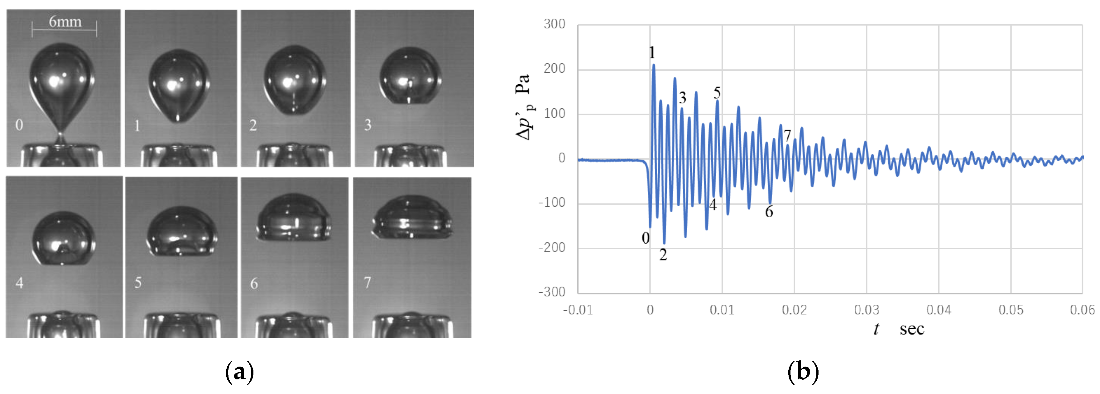
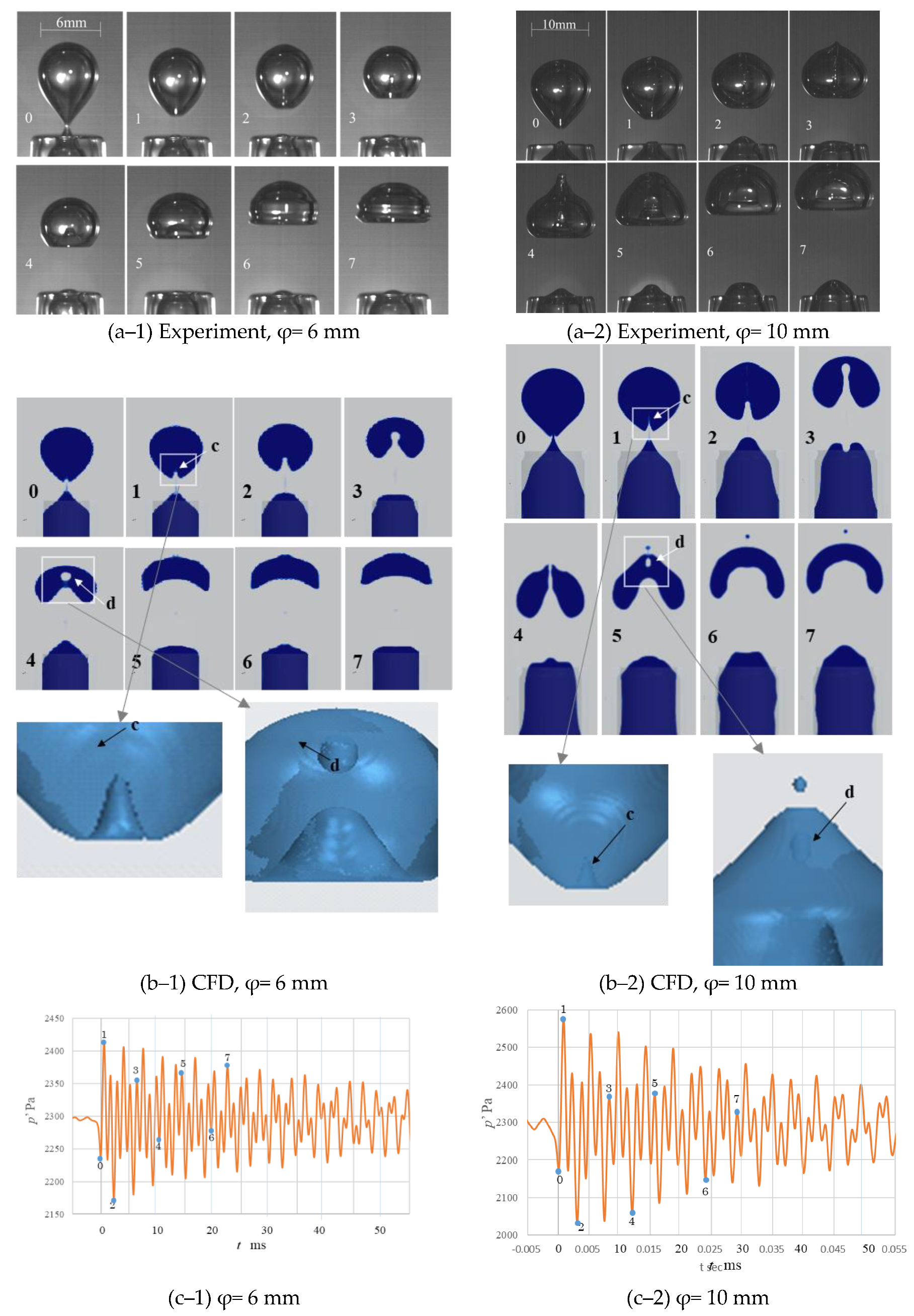
2.2. Overview of Experimental Results

The experimental values are shown in

Table 1. Experimental conditions.

φ mm	$R^{*}$ mm	$v$ m/s	Re	Eo
4	3.2	0.24	7.7 × 102	1.39
6	3.5	0.19	6.6 × 102	1.66
8	4.8	0.17	8.1 × 102	3.13
10	5.0	0.17	8.5 × 102	3.39

, and Figure 2 shows the exemplary results of the bubble deformation images acquired with the high-speed camera and pressure waveform measured by using the hydrophone. The experimental conditions were as follows: φ = 6 mm and supply air flow rate, Q = 0.186 mL/s. The labeled numbers from 0–7 shown in Figure 2a correspond to the sampling times in Figure 2b. Here, the frame rate of the high-speed video camera is 2 kHz, and the hydrophone is 40 kHz. Photograph observation and pressure waveform recordings were recorded synchronously by using a laser trigger signal as shown in Figure 1, and these were correlated based on the time recording. The deformation of a bubble shape rising in water was inspected by Clift et al. [26]. They observed the deformation as spherical, ellipsoidal, and spherical-cap types, which were classified in terms of the Reynolds and Eötvös numbers.

$$Re=\frac{{\rho }_w{R}^{*}v}{{\mu }_w}$$

(1)

$$Eo=\frac{g({\rho }_w-{\rho }_a)R^{*2}}{\sigma }$$

(2)

Additionally, in the deformation process described in the report [26], the bubble configuration was spherical like a balloon at the moment of detachment, deformed to ellipsoidal or wobbling, and finally, was a spherical-cap shape through rising under the present experimental conditions. Preliminarily, according to his classification, we checked all deformation processes in the present experiment. From the flow visualization, it was confirmed that the current results qualitatively followed the classification performed in the aforementioned study.

As shown in the pressure waveform in Figure 2b, a negative pressure drop $\Delta p_p^{\prime }$ appeared when the bubble was detached from the nozzle, as is indicated at the time index number “0”, i.e., t = 0 ms. Thereafter, a damped oscillation started. $\Delta p_p^{\prime }$ should be determined by the critical balance of the forces with the buoyancy force and surface tension, and therefore, in this case, $\Delta p_p^{\prime }$ was detected as approximately −150 Pa, as the output of the hydrophone and the oscillation attenuated within 60 ms. The waveform does not show a monotonous damped oscillation, such as a single discrete frequency oscillation; instead, it seems to involve multiple frequencies. The additional frequencies may be attributed to the higher oscillation modes of the bubble interface or the interactions between the external boundaries.

The primary frequency was obtained via an FFT analysis, which is plotted for the bubble diameter 2R* in Figure 3. 2R* was scattered because the bubble release was very sensitive to experimental conditions, such as the discharge air flow rate, water surface disturbance, and the influence of pre-release bubble behavior. As shown in this figure, one can see that the primary frequency as the breathing mode agrees well with the natural frequency by the following Equation (3). Under the assumption of isentropic change of air bubbles, in this equation, we assume $\gamma =\kappa$.

$$f=\frac{1}{2\pi R^{*}\sqrt{{\rho }_w}}\sqrt{3\gamma p_{\infty }-\frac{2\sigma }{R^{*}}}$$

(3)

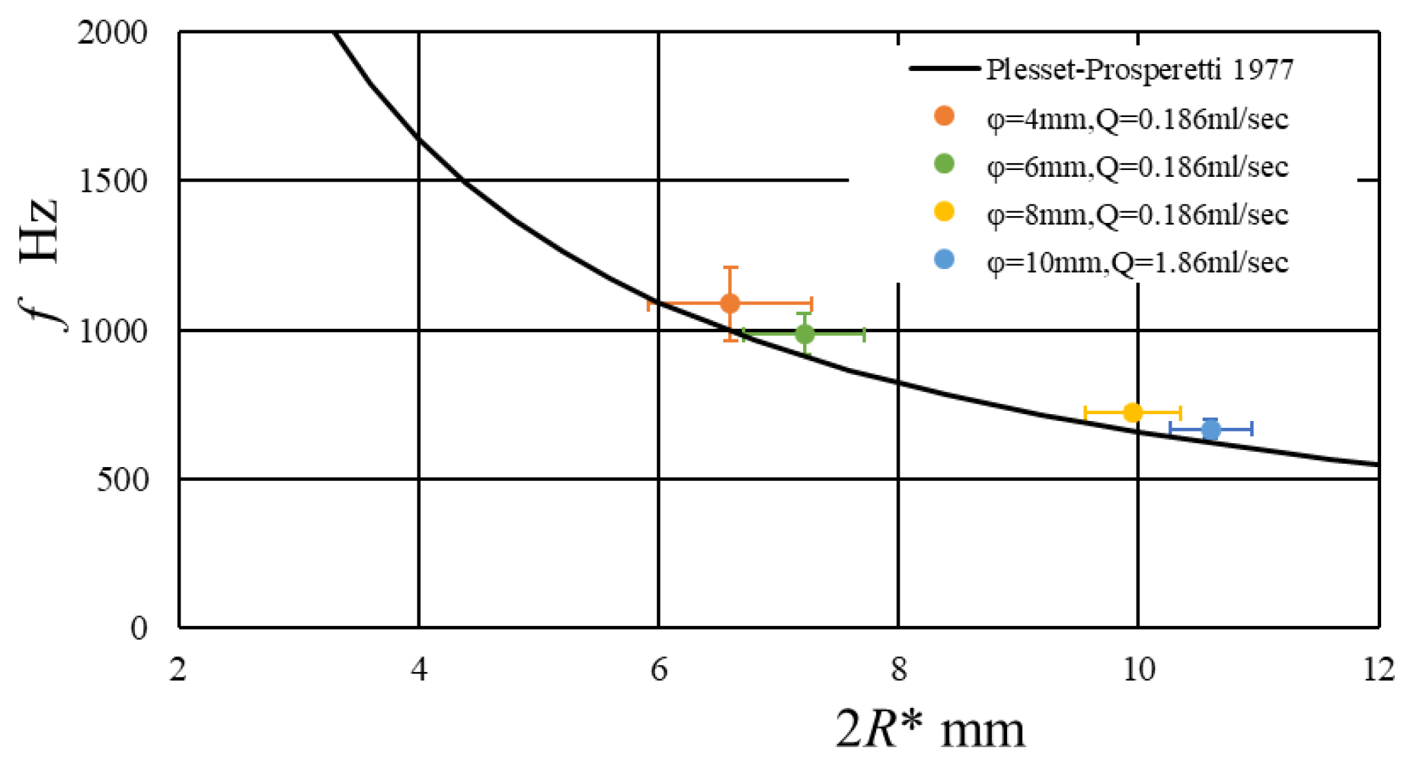
3. Vibrational Motion in the Breathing Mode

The conventional analysis of bubble motion, which is based on the Rayleigh-Plesset Equation (4) [5,27], is now considered This well-known equation describes the bubble motion in a spherical coordinate for compressible air and incompressible water.

$$R\ddot{R}+\frac{3}{2}{\dot{R}}^2=\frac{1}{{\rho }_w}\left[p_{i,eq}{\left(\frac{R^{*}}{R}\right)}^{3\gamma }-p_{\infty }-\frac{2\sigma }{R}-4\mu \frac{\dot{R}}{R}\right]$$

(4)

where, $R$, $\dot{R}$, and $\ddot{R}$ are the bubble radius, velocity, and acceleration, respectively. Here, $\gamma =\kappa$ again, for the usual situation. The brace of the right-hand side of this equation represents the pressure variation of the water, $\Delta p$, near the bubble. $p_{ieq}$ is the pressure inside the bubble at an equilibrium state. The first term in the brace represents the pressure contribution corresponding to an adiabatic change of the bubble. We can obtain $p_{i,eq}=p_{\infty }+2\sigma /R^{*}$ for $R$ = $R^{*}$ for the rest state. The third and fourth terms in the brace are the Laplace pressure and viscous pressure contribution, respectively. To determine a simple or initial problem of bubble oscillation, the initial pressure condition corresponding to bubble detachment was considered. Namely, we have to determine the initial pressure drop $\Delta p_p$ at t = 0 in Figure 2b. The initial pressure $\Delta p_p$ when the bubble detaches is as follows:

$$\left(p_{\infty }+\frac{2\sigma }{R^{*}}\right)\left({\left(\frac{R^{*}}{R_{\max }}\right)}^{3\gamma }-1\right)=\Delta p_p$$

(5)

We deduced the pressure drop from the experimental pressure record in Figure 2b. The pressure amplitude is attenuated spherically through wave propagation, with a function being inversely proportional to the radial distance $r$ [12,28]. According to the theoretical analysis so far, it is necessary to consider the effect of the changes in the pressure field in proportion to the −2 and −4 powers of the radial distance $r$ and with the dynamic pressure based on $\dot{R}$. In the present case, the influence of this additional higher term resulted in less than a few pascals. Therefore, we approximate the pressure $\Delta p$ with the following equation, which is inversely proportional to the distance. For $r=R^{*}$ and $d$, we can estimate the pressure variation in the vicinity of the bubble, $\Delta p$ using the following simple equation:

$$\Delta p=\frac{d}{R^{*}}\Delta p^{\prime }$$

(6)

For a given $R^{*}$ and $\Delta p_p$, we obtained the radius amplitude of the oscillation $\Delta R=R-R^{*}$ from Equation (4), as shown in

Table 2. Estimated pressure drop and radius variation.

φ mm	R* mm	Images	d mm	Δp′p Pa	Δpp Pa	ΔR by Equation (4) μm
4	3.2		18	−86	−480	±3.2
6	3.5		17	−152	−740	±5.7
8	4.8		16	−270	−900	±9.9
10	5.0		16	−329	−1050	±11.9

and Figure 4. For instance, in the case of φ = 6 mm because the representative radius $R^{*}$ was 3.5 mm, $d$ = 17 mm at the moment in the experiment and $\Delta {p^{\prime }}_p$ = −150 Pa, as indicated at point 0 in Figure 2b, we obtained $\Delta p_p$ = −740 Pa from Equation (6). The radius amplitude became 5.7 μm, as shown in Figure 4.

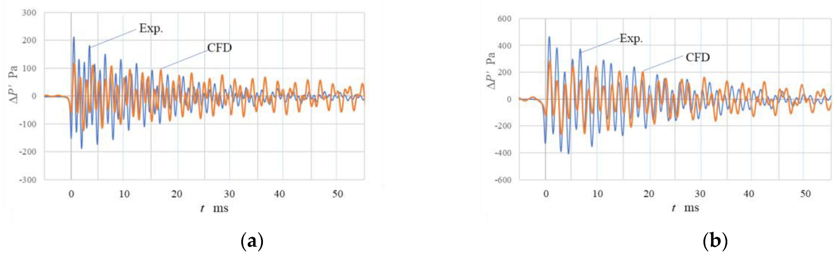
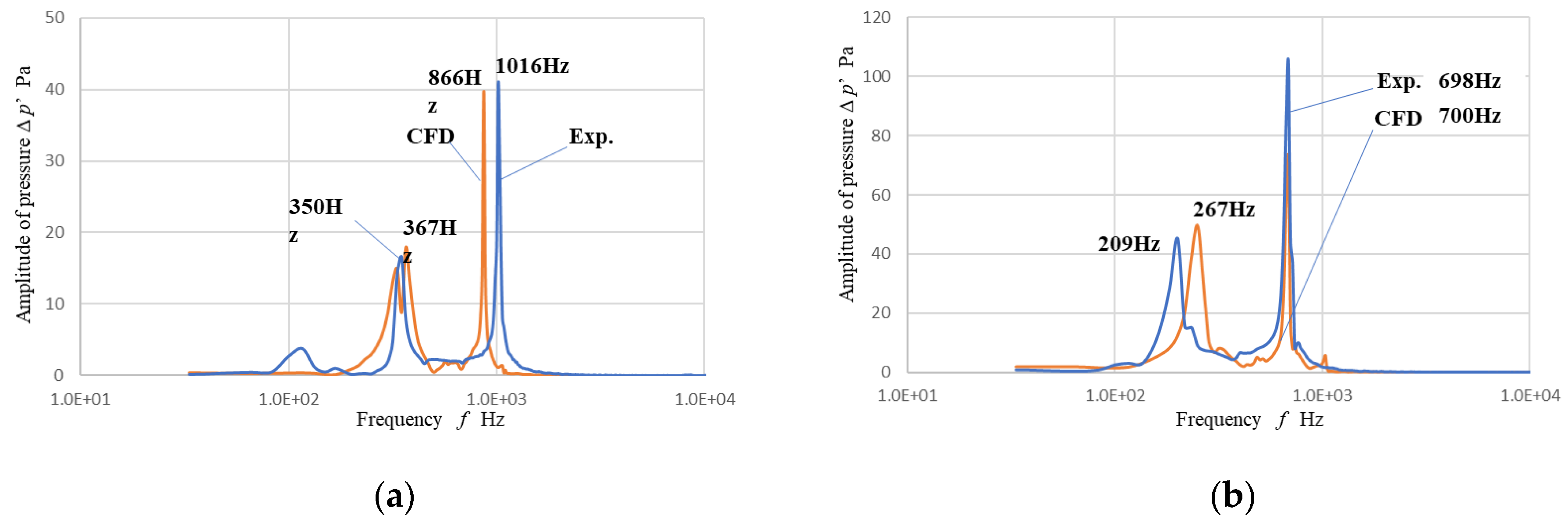
4. Computational Fluid Dynamics Simulation

4.1. Governing Equation and Scheme

To simulate the present problem, we solved a set of mass conservation equations, the compressible Navier-Stokes equation, and energy conservation equations in 3D coordinate for air and water simultaneously; specifically, a consistent finite volume differential scheme was applied for air and water. The interface between air and water was determined using the VOF method with a high-resolution interface capturing (HRIC) scheme [29]. The set of these equations is expressed as follows:

$$\frac{\partial \rho }{\partial t}+\frac{\partial }{\partial x_j}(\rho u_j)=0$$

(7)

$$\frac{\partial }{\partial t}\rho u_i+\frac{\partial }{\partial x_j}\rho u_i{u}_j=\rho g_i-\frac{\partial p}{\partial x_i}+\frac{\partial }{\partial x_j}(\mu (\frac{\partial u_i}{\partial x_j}+\frac{\partial u_j}{\partial x_i}-\frac{2}{3}\frac{\partial u_k}{\partial x_k}{\delta }_{ij}))-\rho \left(\frac{\partial n_k}{\partial x_k}\right)n_i\sigma$$

(8)

$$\frac{\partial }{\partial t}\rho e+\frac{\partial }{\partial x_j}\rho e{u}_j=\frac{\partial }{\partial x_j}(\lambda \frac{\partial T}{\partial x_j})-p\frac{\partial u_j}{\partial x_j}+\Phi$$

(9)

$$\frac{\partial \alpha }{\partial t}+u_j\frac{\partial \alpha }{\partial x_j}=0$$

(10)

where $\rho$, $u$, $p$, and $e$ are the density, velocity, pressure, and internal energy, respectively. $\lambda$ and $\Phi$ are the thermal conductivity and energy dissipation function, respectively. The scaler value of the VOF, $\alpha$ is tracked using the scalar transfer equation shown in Equation (10). $\alpha$ is 0 for water and 1 for air. The variable $n_i$ used in Equation (8) represents a normal unit vector on the interface between air and water, which is expressed in terms of $\partial \alpha /\partial x_i$. This term should vanish, except along the interface.

The set of equations was solved using a three-dimensional Euler multiphase model and the VOF method, using Star-CCM+. The air is assumed to be an ideal gas, and the state of water was determined using the table provided by the International Association for the Properties of Water and Steam (IAPWS)-IF 97. The convection terms are discretized with a second order upwind scheme and time integration is second-order SIMPLE algorithm. No turbulence model was used. The time increment Δt was 25 μs, which ensured a pressure measurement resolution of 40 kHz in the experiment. The other practical constant used in this simulation is described in the following section.

4.2. Computational Parameters and Mesh Validation

In this simulation, the bubble detachment accompanied an impulse that was a discontinuous force generation at pinch-off (detachment). The present simulation should be interpreted as an initial value problem mathematically, which was determined by the bubble detachment condition. The present simulation was conducted in a 3D coordinate for the general discussion without any simplification such as axisymmetric assumption. We simulated the detachment process automatically, so the force at pinch-off was occupied by the bubble size, surface tension, and growth rate of the bubble. Furthermore, the bubble detachment was influenced by the configuration of the nozzle exit. As shown in Figure 5a, the nozzle was placed 250 mm deep in a cylindrical water tank. We reproduced the configuration of the nozzle exit in the simulation as precisely as the experimental one (Figure 5b). For the mesh size validation, we examined the mesh size allowance to obtain a reasonable resolution by comparing the pressure signal. Here, polyhedral cells were used in the simulation. After the trials and improvements, we focused on the cell size near the nozzle and bubble. The present calculation consumed a big storage and huge time, we had to determine the reasonable cell size to secure the accuracy.

In the preliminary benchmark tests, we checked this influence by using 250, 200, 150, and 120 μm cell sizes for the mesh system, similar to that in Figure 5b, in which a spherical bubble vibration with ±1, 2, 3, 5, and 10 μm initial displacements was demonstrated for the four cell sizes stated above. In this assessment, we confirmed the accuracy of less than 10% of the displacements was assured for 150 μm and 120 μm cell sizes. Finally, we used two cell sizes of 150 μm and 120 μm near the bubble on the last cell size examination shown in Figure 5b. The simulation was conducted using 140 cores of Intel Xeon X7542. The elapsed time was 540,000 s for a 150 μm cell size, and 1,330,000 s for 120 μm. The pressure difference was less than several percent. Finally, the necessary total cell number was 18 M cells of the polyhedral grid. Figure 5b shows the cell refinement around the nozzle. The fundamental cell size was 150 μm near the nozzle, which is 1/40 of the nozzle diameter. The boundary condition of the tank is nonslip, and the upper surface had a free surface condition.

Next, the consideration of the water surface contact angle is a difficult problem in multi-phase simulations. The contact angle is usually 40°–45° on the static interface, which was confirmed by the capillary-reservoir method for different inner diameters of the nozzle. However, there are some discussions about the dynamic contact angle [30], which should be verified in physical modeling. In the present simulation, we determined the appropriate angle by trial and error. The resultant value was 9° through the detachment process. Furthermore, we observed the capillary waves on the surfaces after detachment not only on the bubble but also on the air column in the nozzle. A similar disturbance on the water surface is so sensitive that we had to take care of the starting air charge to avoid the incidence of the initial disturbance. Therefore, the air charge rate gradually increased to the target rate just after the start of the simulation.

Third, we should note the effect of compressibility in CFD. Since our aim is to discuss the breathing mode oscillation, we took the compressibility into account for both fluids, as presented in the previous section. In our simulation, the acoustic Courant number C_a in water became 250 if Δt = 25 μs, and the minimum mesh size was 150 μm. After carried out, supplemental studies in the same mesh system in Figure 5b during one cycle oscillation of breathing mode for Δt = 12.5, 5, 2.5, 1.25, and 0.1 μs, i.e., C_a = 125, 50, 25, 12.5, and 1, we confirmed that the deviation of pressure variation and frequency was less than 3% in the breathing mode oscillation.

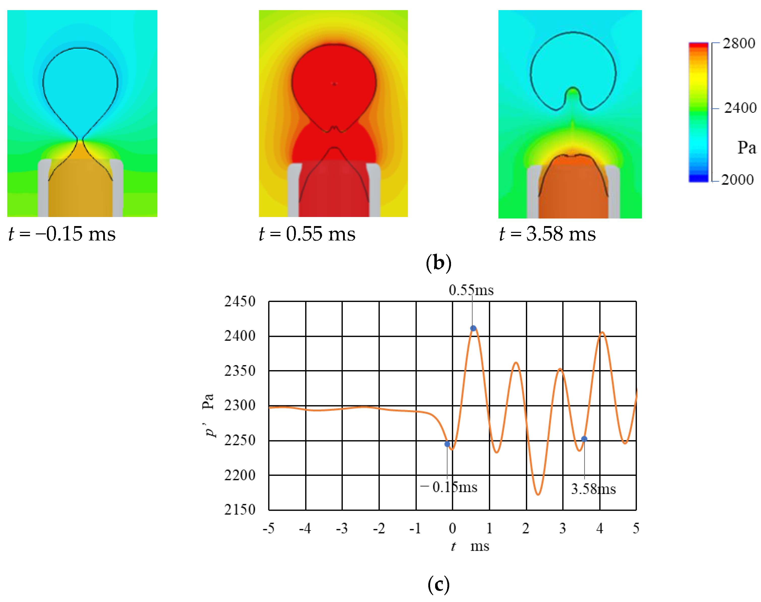
4.3. Overview of Density and Pressure Change

Figure 6 demonstrates the typical results of the CFD simulation for φ = 6 mm. Here, a couple of instantaneous distributions of (a) density and (b) pressure are illustrated at −0.15, 0.55, and 3.58 ms after detachment. Figure 6c shows the pressure diagram, in which the corresponding sampling period is indicated.

The state at t = −0.15 ms indicates just before the bubble release, where we can see a narrowing waist. The density and pressure decrease slightly relative to the initial state. After the bubble release, at t = 0.55 ms, the shrinking waist and rising plume were observed, and both the density and pressure increased in a short period. As shown in Figure 6c, the pressure has a maximum value at t = 0.55 ms because the natural frequency is approximately 1 kHz, and the period is approximately 1 ms. At t = 3.58 ms, the state indicates the negative pressure phase after three vibration cycles. As illustrated in these images, whereas we can recognize the oscillatory behavior in density and pressure, the distribution is almost uniform inside the bubble. Therefore, it was found that the oscillation was dominated by the breathing mode.

4.4. Deformation and Pressure Diagram for Long-Term

The bubble deformation photos in the experiment and images obtained by CFD are shown for several tenths of a millisecond in Figure 7. The bubble images were illustrated by the threshold between air and water, which is α = 0.5. Comparing these photos and images, the deformation process showed a good agreement with the experimental results. Figure 7(c–1) and (c–2) show the pressure profile after bubble detachment. The labeled numbers 0–7 in Figure 7(a–1), (b–1), and (c–1), and Figure 7(a–2), (b–2), and (c–2) show the corresponding sampled times, respectively. After the detachment of the bubble, the cusp at the bottom suddenly rebounded upwards, and the reversed cusp of water is found as shown as symbol “c” in Figure 7(a–2) time-1 and (b–2) time-1. The cusp deformed and a tiny liquid droplet was observed in the bubble, as indicated by the symbol “d” in Figure 7(b–1) time-4 and Figure 7(b–2) time-5, respectively. As shown in these figures, the bubble shows considerable deformation accompanying the capillary wave propagation. However, such visible deformation is essentially unrelated to sound emission. We will discuss the sound generation due to the breathing mode later in this study. However, the bubble deformation is dynamic and complicated. In the present simulation, the VOF interface diffused slightly through the calculation. However, the interface is sufficiently preserved during deformation. Thus, we can observe not only the capillary waves but also the droplet penetration.

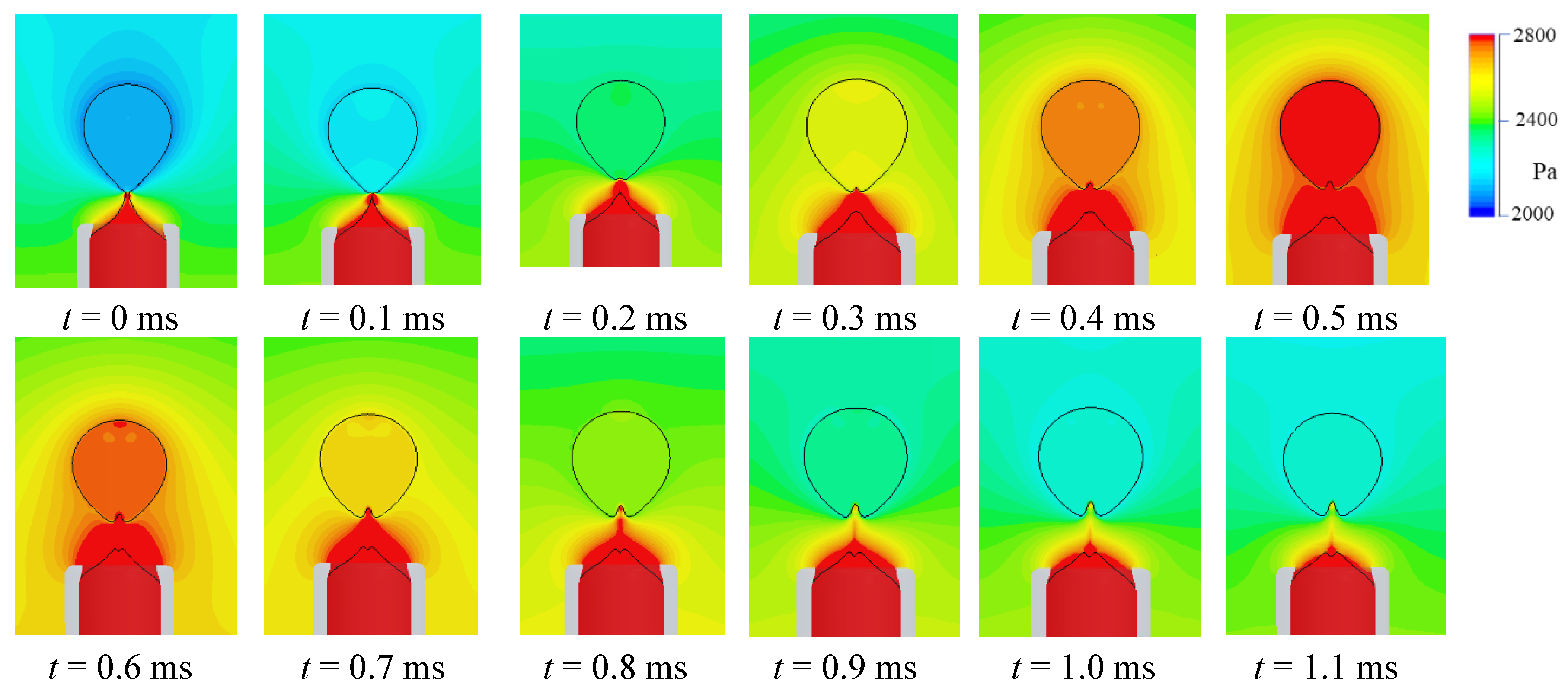
4.5. Pressure Distribution for One Cycle

Figure 8 shows the time-sequential pressure distribution during one cycle of oscillation from t = 0–1.1 ms for ϕ = 6 mm. The sequence of the pressure change is quite interesting to consider the sound emission at the bubble detachment. From these figures, it is apparent that the pressure has the minimum inside and near fields of the bubble at t = 0 ms, the pressure inside the nozzle, including the water and air, has a larger pressure. The pressure distribution appears to be a dipole. After detachment, the bubble pressure rapidly increased, and the coupled pressure jump was generated at t = 0.5 ms. One can recognize the resonant process at this moment. However, the pressure oscillations of the bubble and nozzle air had a different oscillatory mode thereafter. In all simulations for different conditions, we confirmed that the pressure was maximum at the timing of “1”. At a pressure drop at time “0” s, $\Delta p_p$ was rigorously sensitive to the exact representation of the interface. Furthermore, the maximum peak pressure depended considerably on the geometry and boundary conditions of the water tank, nozzle geometry, and position for both the experiment and numerical simulation. In future works, it is suggested that we should take care of these computational conditions.

Figure 9 shows the comparison of the pressure at the measuring point between the experiment and CFD. The result obtained by CFD shows a similar oscillatory curve as the experimental one. From a quantitative viewpoint, the amplitude is of the same order, but lower and not more attenuated than that of the experimental one. First, regarding this problem, we have to take note of the initial pressure drop, $\Delta p_p^{\prime }$. This magnitude depends on the condition of the bubble detachment, as mentioned in the previous section. To obtain a pressure drop as accurate as the experimental one, we had to use finer meshes and reasonable interface representation in the simulation by using a larger computer resource.

Second, at the positive overpressure succeeding to the pinch-off, the amplitude of the positive pressure is much larger than that of the initial pressure drop for all initial conditions. The pressure distribution at t = 0.5 ms in Figure 8 corresponds to this situation. As illustrated in this figure, the pressure in the bubble is influenced by the vibration of the air column. Although we can recognize the local pressure distribution around the bubble, the surrounding boundary condition like eigenmode of tank water may affect the pressure variation of the breathing mode of the bubble.

Next, the experimental result shows a large attenuation rate. The attenuation may depend on acoustic dissipation due to impurities in water or the influence of sub-micron bubbles resolved in the water, but it is not yet clear.

The spectrum of the pressure variation is shown in Figure 10. This figure depicts the pressure amplitude calculated by using FFT analysis for the experimental and CFD results for 60 ms. The natural frequency strongly depends on the initial radius of the bubble. Owing to the dependency of the natural frequency f on $R^{*}$, the experimental frequency was approximately 15% higher than that of CFD for φ = 6 mm, and almost the same frequency for ϕ = 10 mm for the primary one. Secondary frequency peaks were observed around 350 and 367 Hz in Figure 10a and 209 and 267 Hz in Figure 10b, respectively. This low frequency oscillation may be influenced by the coupling of the oscillation of the bubble and air in the nozzle. Furthermore, we should consider the ambient water effect, which is mentioned as the “dressed” bubble, as expressed in Ref [13].

There have been many investigations on the acoustic field in multi-phase flow. For example, a relevant investigation was carried out by Manasseh et al. [14,31] for bubble coalescence and Leighton et al. [32] for the reverberation of the damping bubbles. For the low-frequency oscillation, the interaction of the breathing mode of the bubble and air column in the nozzle was discussed by changing the nozzle length to 10, 20, and 40 mm in CFD. The results are shown in Figure 11 and Figure 12. Apparent interactions were observed in the pressure diagram due to the resonance of the air column in the nozzle. The longer the nozzle length, the lower the second frequency. As discussed in the previous section, not only does the interaction between the breathing mode of the bubble and air column play an important role on the pinch-off impulse, the interaction also influences the successive process by superimposing the acoustic field.

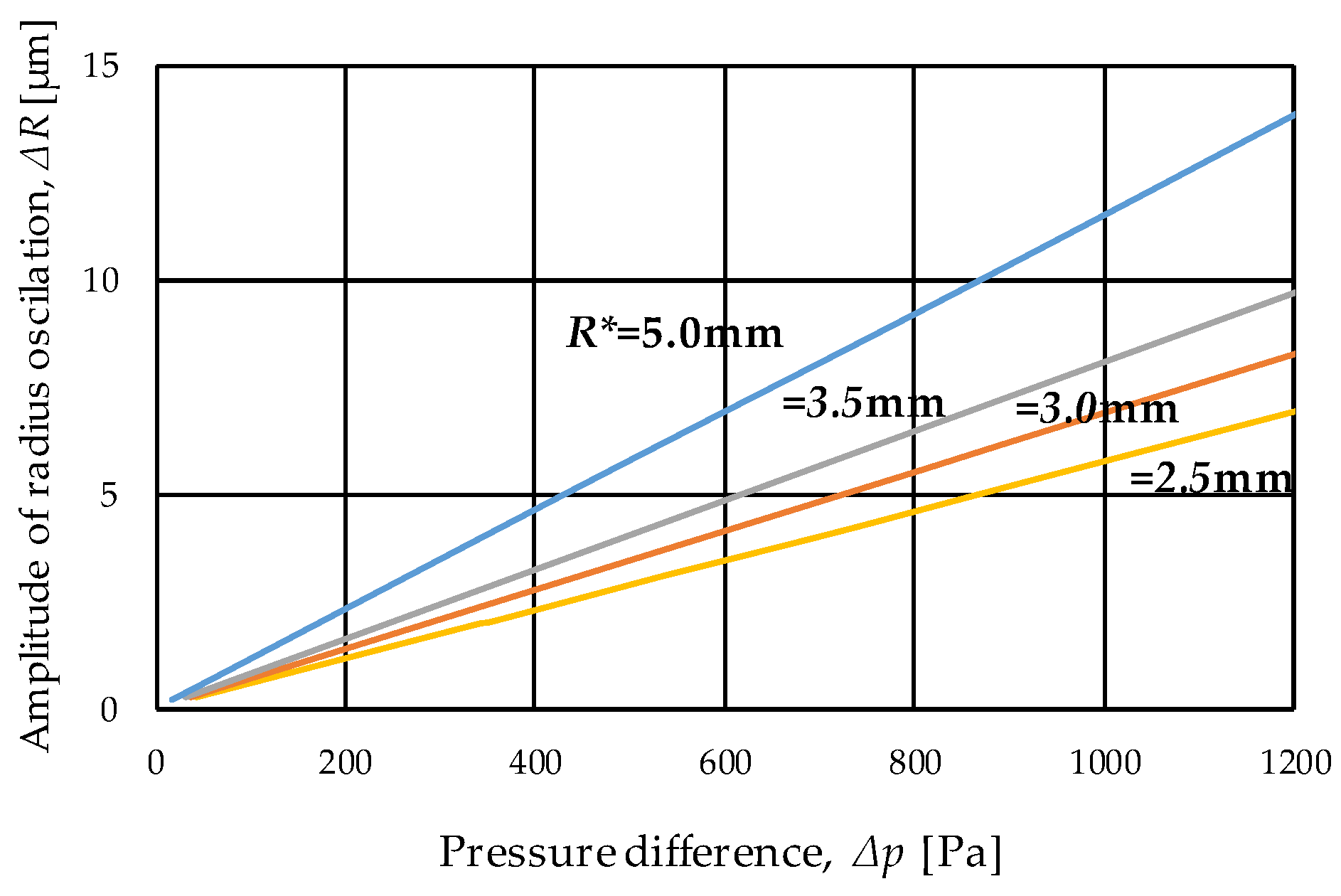
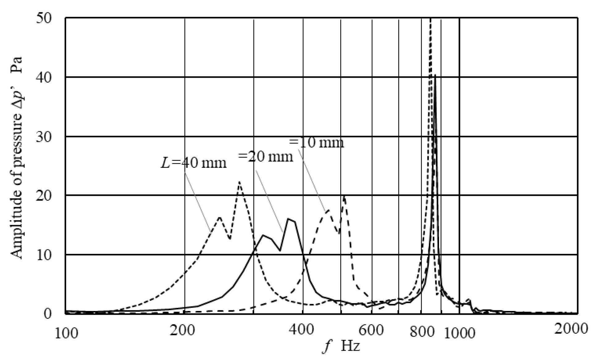
4.6. Radial Variation in the Breathing Mode

In the present computation, we have succeeded in expressing the volumetric oscillation of the breathing mode by using the VOF method with adequate accuracy. In previous studies, one can find a bubble deformation simulation using VOF, but almost no previous study discussed volumetric vibration. Wu et al. demonstrated volume evolution before and after bubble detachment [33]. Unfortunately, we could not find the oscillation process after detachment. As described in Section 4.1, to obtain a reasonable solution for the bubble deformation process, we used a 150 μm cell size in the region of interest. The approximated cell number in this region of interest reached up to 1 M cells. To discuss the amplitude of the radius variation, the volume of the bubble was integrated according to the α-value. By integrating the volume where α > 0 over the whole field, an equivalent radius was estimated.

Figure 13 illustrates the variation of the bubble radius and the pressure at the hydrophone’s position for the case of φ = 6 and 10 mm. The integration should have been started immediately after detachment, but it was started after a certain short time to avoid a rapid bubble deformation process involving the pinch of detachment. As shown in this figure, the frequency of the radius variation is completely synchronized with the pressure fluctuation. Therefore, the radius variation indicates the influence attributed to the breathing mode. As the bubble rises with time, the mean radius increases because of the decrease in static pressure. Here, the magnitude of the radius oscillation is approximately 3.0 and 4.2 μm for φ = 6 and 10 mm, respectively.

The radius variation once more in terms of the given initial pressure change by using Equation (4) is discussed. As described in the previous chapter, the initial pressure was $\Delta p_p^{\prime }$ = −150 Pa and $\Delta p_p$ = −730 Pa for φ = 6 mm. On the other hand, the numerical value of the pressure drop at the hydrophone $\Delta p_p^{\prime }$ was −60 Pa in Figure 9, so the corresponding $\Delta p_p$ in CFD was −290 Pa. From the solution in Figure 4, the amplitude of the radial oscillation in the breathing mode becomes 2.4 μm for R* = 3.5 mm and $\Delta p_p$ = 290 Pa. That is, the relation between the radius oscillation ΔR and the pressure Δp in CFD shows good agreement with the Rayleigh-Plesset equation. However, we still have a significant disagreement $\Delta p_p$ between the experiment and numerical simulation. We expect a sharp and large pressure drop by improving the cell structure with finer cell size. Concludingly, it was found that the present simulation provided a sufficient solution for the relation between the bubble radius and pressure variation for a given initial pressure drop.

5. Conclusions

Sound emission at bubble detachment from the nozzle in water was studied experimentally and numerically. The two-phase flow was simulated with the finite volume method and the VOF method, which was adopted to express the interface between the two fluids.

By using the VOF method with moderate fine meshing, it was possible to simulate both bubble deformation and pressure variation after detachment with reasonable accuracy. To reproduce the sound pressure waveform, it was necessary to divide the nozzle surroundings into fine cells of at least 1/40th of the size of the bubble diameter. If the bubble is represented by approximately 1 M cells in such a condition, the simulation results fairly agree with the experimental results. The obtained pressure field showed a peculiar resonance process of sound. The dipole pressure distribution just before bubble detachment was transitioned to a coupled resonant process in a short period after detachment. The spectrum of pressure after detachment indicated a natural frequency of the breathing mode as the first peak and low frequency as the second peak. The pressure distribution after bubble detachment showed a strong interference between the breathing mode of the bubble and the vibration of the air column in the nozzle. Furthermore, the radius variation was estimated in the present CFD results. Although the relationship between the variations of bubble radius and pressure showed good agreement with the theoretical one, the initial pressure drop in CFD was less than the experimental one. To obtain an accurate pressure variation after bubble detachment, using the refined cell structure to control the reproduction of the initial pressure drop is a significantly important factor.

References

1. Watanabe, Y. Analytical study of acoustic mechanism of “suikinkutsu”. Jpn. J. Appl. Phys. Part 1 Regul. Pap. Short Notes Rev. Pap. 2004, 43, 6429–6443. [Google Scholar] [CrossRef]
2. Oku, T.; Hirahara, H.; Akimoto, T. Visualization of deformation and sound emission from bubble in water using VOF method. In Proceedings 18th International Symposium on Flow Visualization; ETH: Zurich, Switzerland, 2018; pp. 1–9. [Google Scholar]
3. Rayleigh, L., VIII. On the pressure developed in a liquid during the collapse of a spherical cavity. Lond. Edinb. Dublin Philos. Mag. J. Sci. 1917, 34, 94–98. [Google Scholar] [CrossRef]
4. Minnaert, M. On musical air-bubbles and the sounds of running water. Lond. Edinb. Dublin Philos. Mag. J. Sci. 1933, 16, 235–248. [Google Scholar] [CrossRef]
5. Plesset, M.S.; Prosperetti, A. Bubble dynamics and cavitation. Annu. Rev. Fluid Mech. 1977, 9, 145–185. [Google Scholar] [CrossRef]
6. Strasberg, M. Gas Bubbles as Sources of Sound in Liquids. J. Acoust. Soc. Am. 1956, 28, 20–26. [Google Scholar] [CrossRef]
7. Longuet-Higgins, M.S. Monopole emission of sound by asymmetric bubble oscillations. Part 1. Normal modes. J. Fluid Mech. 1989, 201, 525–541. [Google Scholar] [CrossRef]
8. Longuet-Higgins, M.S. Monopole emission of sound by asymmetric bubble oscillations. Part 2. An initial-value problem. J. Fluid Mech. 1989, 201, 543–565. [Google Scholar] [CrossRef]
9. Longuet-Higgins, M.S.; Lunde, K. The release of air bubbles from an underwater nozzle. J. Fluid Mech. 1991, 230, 365–390. [Google Scholar] [CrossRef]
10. Oguz, H.N.; Prosperetti, A. Dynamics of Bubble Growth and Detachment from a Needle. J. Fluid Mech. 1993, 257, 111–145. [Google Scholar] [CrossRef] [Green Version]
11. Oğuz, H.N.; Prosperetti, A. The natural frequency of oscillation of gas bubbles in tubes. J. Acoust. Soc. Am. 1998, 103, 3301–3308. [Google Scholar] [CrossRef]
12. Leighton, T.G. The Freely-oscillating Bubble. In The Acoustic Bubble; Academic Press: London, UK, 1994; pp. 129–286. [Google Scholar]
13. Devaud, M.; Hocquet, T.; Bacri, J.; Leroy, V.; Devaud, M.; Hocquet, T.; Bacri, J.; Leroy, V. The Minnaert bubble: A new approach. To cite this version: HAL Id: Hal-00145867. Available online: https://hal.archives-ouvertes.fr/hal-00145867 (accessed on 14 May 2007).
14. Manasseh, R.; Riboux, G.; Bui, A.; Risso, F. Sound emission on bubble coalescence: Imaging, acoustic and numerical experiments. In Proceedings of the 16th Australian Fluid Mechanics Conference, 16AFMC, Crown Plaza, Gold Coast, Australia, 2–7 December 2007; pp. 167–173. [Google Scholar]
15. Czerski, H.; Deane, G.B. Contributions to the acoustic excitation of bubbles released from a nozzle. J. Acoust. Soc. Am. 2010, 128, 2625–2634. [Google Scholar] [CrossRef] [PubMed]
16. Phillips, S.; Agarwal, A.; Jordan, P. The Sound Produced by a Dripping Tap is Driven by Resonant Oscillations of an Entrapped Air Bubble. Sci. Rep. 2018, 8, 1–12. [Google Scholar] [CrossRef] [PubMed]
17. di Bari, S.; Robinson, A.J. Experimental study of gas injected bubble growth from submerged orifices. Exp. Therm. Fluid Sci. 2013, 44, 124–137. [Google Scholar] [CrossRef] [Green Version]
18. Van Sint Annaland, M.; Deen, N.G.; Kuipers, J.A.M. Numerical simulation of gas bubbles behaviour using a three-dimensional volume of fluid method. Chem. Eng. Sci. 2005, 60, 2999–3011. [Google Scholar] [CrossRef]
19. Quan, S.; Hua, J. Numerical studies of bubble necking in viscous liquids. Phys. Rev. E Stat. Nonlinear Soft Matter Phys. 2008, 77, 1–11. [Google Scholar] [CrossRef]
20. Hanafizadeh, P.; Eshraghi, J.; Kosari, E.; Ahmed, W.H. The effect of gas properties on bubble formation, growth, and detachment. Part. Sci. Technol. 2015, 33, 645–651. [Google Scholar] [CrossRef]
21. Ambrose, S.; Hargreaves, D.M.; Lowndes, I.S. Numerical modeling of oscillating Taylor bubbles. Eng. Appl. Comput. Fluid Mech. 2016, 10, 578–598. [Google Scholar] [CrossRef] [Green Version]
22. Xi, W.Q. Numerical simulation of violent bubble motion. Phys. Fluids 2004, 16, 1610–1619. [Google Scholar] [CrossRef] [Green Version]
23. Bui, A.; Manasseh, R. A CFD Study of the Bubble Deformation during Detachment. In Proceedings of the Fifth International Conference on CFD in the Process Industries, CSIRO, Melbourne, Australia, 13–15 December 2006; pp. 1–6. [Google Scholar]
24. Liu, J.; Chu, N.; Qin, S.; Wu, D. Acoustic analysis on jet-bubble formation based on 3D numerical simulations. In Proceedings of the INTER-NOISE 2016—45th International Congress and Exposition on Noise Control Engineering: Towards a Quieter Future, Hamburg, Germany, 21–24 August 2016; pp. 5103–5111. [Google Scholar]
25. Liu, J.; Chu, N.; Qin, S.; Wu, D. Numerical simulations of bubble formation and acoustic characteristics from a submerged orifice: The effects of nozzle wall configurations. Chem. Eng. Res. Des. 2017, 123, 130–140. [Google Scholar] [CrossRef]
26. Clift, R.; Grace, J.R.; Weber, M.E. Bubbles, Drops and Particles; Academic Press: Cambridge, MA, USA, 1978; Volume 61, ISBN 012176950X. [Google Scholar]
27. Prosperetti, A. Bubble phenomena in sound fields: Part one. Ultrasonics 1984, 22, 69–77. [Google Scholar] [CrossRef]
28. Vokurka, K. On Rayleigh’s model of a freely oscillating bubble. I. Basic relations. Czechoslov. J. Phys. 1985, 35, 28–40. [Google Scholar] [CrossRef]
29. Muzaferija, S.; Peric, M. Computation of free-surface flows using interface-tracking and interface-capturing methods. In Nonlinear Water Waves Interaction; WIT Press: Alpha House, UK, 1999. [Google Scholar]
30. Islam, M.T.; Ganesan, P.; Sahu, J.N.; Hamad, F.A. Numerical study to investigate the effect of inlet gas velocity and Reynolds number on bubble formation in a viscous liquid. Therm. Sci. 2015, 19, 2127–2138. [Google Scholar] [CrossRef] [Green Version]
31. Manasseh, R.; Riboux, G.; Risso, F. Sound generation on bubble coalescence following detachment. Int. J. Multiph. Flow 2008, 34, 938–949. [Google Scholar] [CrossRef]
32. Leighton, T.G.; White, P.R.; Morfey, C.L.; Clarke, J.W.L.; Heald, G.J.; Dumbrell, H.A.; Holland, K.R. The effect of reverberation on the damping of bubbles. J. Acoust. Soc. Am. 2002, 112, 1366–1376. [Google Scholar] [CrossRef] [PubMed]
33. Wu, W.B.; Liu, Y.L.; Zhang, A.M. Numerical investigation of 3D bubble growth and detachment. Ocean Eng. 2017, 138, 86–104. [Google Scholar] [CrossRef]
Figure 1. Experimental apparatus.
Fluids 05 00096 g001
Figure 2. Typical deformation of bubble detachment and the corresponding pressure waveform in the experiment. The nozzle inner diameter, φ = 6 mm and air flow rate, Q = 0.186 mL/s. (a) Flow visualization of bubble detachment. (b) Experimental pressure signal by hydrophone.
Fluids 05 00096 g002
Figure 3. Relation of primary frequency with bubble diameter.
Fluids 05 00096 g003
Figure 4. Amplitude of radial oscillation and pressure estimated by Equation (4).
Fluids 05 00096 g004
Figure 5. Computational grid. (a) Water tank and nozzle. (b) Detail of mesh around the nozzle.
Fluids 05 00096 g005
Figure 6. Density and pressure variation in computational fluid dynamics (CFD), φ = 6 mm. (a) Density of water and air bubble. (b) Pressure. (c) Data sampling timing on pressure diagram at measuring point.
Fluids 05 00096 g006aFluids 05 00096 g006b
Figure 7. Bubble deformation process. (a) Photo images in experiment. (b) Bubble deformation in CFD. (c) Pressure profile of CFD.
Fluids 05 00096 g007
Figure 8. Pressure distribution from the bubble detachment for one cycle for φ = 6 mm.
Fluids 05 00096 g008
Figure 9. Comparison of pressure profile at the position of the hydrophone. (a) φ = 6 mm. (b) φ = 10 mm.
Fluids 05 00096 g009
Figure 10. Spectrum of pressure amplitude. (a) φ = 6 mm. (b) φ = 10 mm.
Fluids 05 00096 g010
Figure 11. Pressure diagram for the nozzle lengths, L = 10, 20, and 40 mm. (a) L = 10 mm. (b) L = 20 mm. (c) L = 40 mm.
Fluids 05 00096 g011
Figure 12. Spectrum of pressure amplitude for the nozzle lengths, L = 10.20, and 40 mm.
Fluids 05 00096 g012
Figure 13. Radius variation of bubble and pressure profile at the measuring point. (a) φ = 6 mm. (b) φ = 10 mm.
Fluids 05 00096 g013