1. Introduction
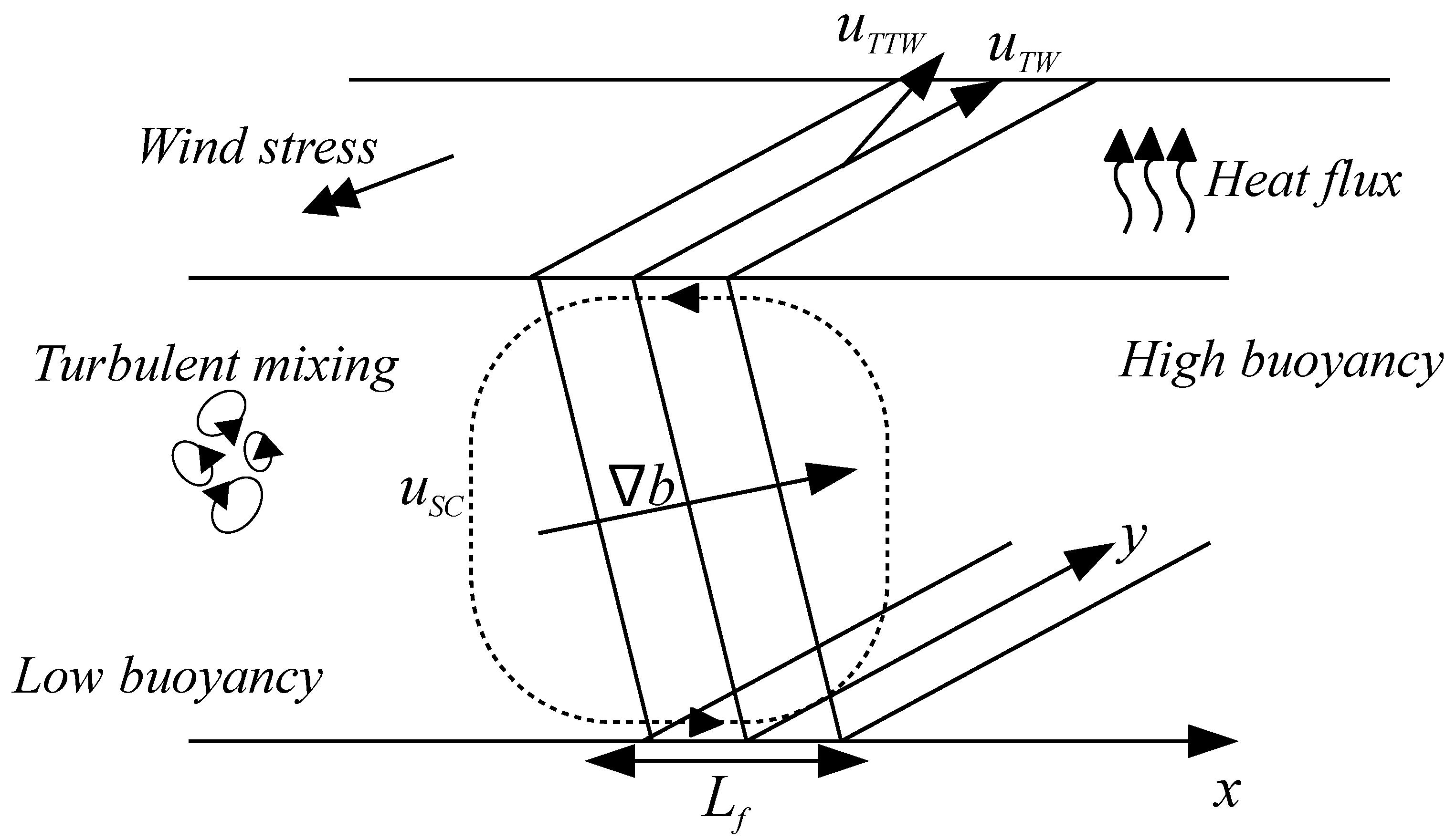
Fronts, or regions of large horizontal density gradient are important features of the upper ocean and atmosphere where they play an important role in the exchange of heat, carbon, and other important tracers. Fronts are highly anisotropic features where the cross-front width (in the direction of the density gradient) is small compared to the along-front length. Fronts can be characterised by their cross-front width which can range from tens of kilometers for large fronts including the Gulf Stream, Kuroshio, and fronts associated with the Antarctic Circumpolar Current (ACC), to scales of meters for fronts associated with freshwater plumes and gravity currents. The focus here will be on relatively large scale fronts where the Rossby number is small and the frontal width is large compared to the mixed layer depth. A typical front is shown in
Figure 1.
The dominant balance in many large-scale frontal systems is between the geostrophic shear and horizontal density gradients, resulting in a balanced state with an along-front ‘thermal wind’ flow [
1]. Elevated levels of small-scale turbulence in the ocean surface mixed layer act to disrupt this balance by driving a circulation around the front which can in turn lead to an intensification of the front (frontogenesis) or spreading of the front (frontolysis) [
2,
3]. Including the effects of vertical mixing in the horizontal momentum equations leads to a state of ‘turbulent thermal wind’ (TTW) or ‘generalised Ekman’ balance, which has been seen in both numerical models of ocean fronts [
3,
4,
5,
6] and observational data [
7].
Frontogenesis is the process by which fronts form and sharpen. Externally imposed strain flows are often used to model the squeezing of fronts by large-scale currents and analytic work by Hoskins and Bretherton [
8] found that for an inviscid front, this external strain flow can lead to a finite-time discontinuity in the surface density. Physically, we expect this collapse to be prevented by the effects of enhanced turbulence and mixing in the frontal region [
9].
Surface wind and buoyancy forcing can have a strong influence on the evolution of ocean fronts. For example, Thomas and Lee [
10] showed that when the surface wind stress is aligned with the thermal wind (in the ‘down-front’ direction), the resulting Ekman flow destabilises the water column resulting in convection, which, combined with Ekman pumping, drives a frontogenetic secondary circulation. This secondary circulation can spontaneously form very sharp fronts and also results in large vertical velocities. Thomas and Ferrari [
11] examined the relative influence of wind-driven circulation and horizontal strain flow on the secondary circulation and stratification at ocean fronts and found that wind-driven circulation can dominate strain-driven frontogenesis for typical ocean conditions.
Surface buoyancy fluxes and wind stresses also act to destabilise vertical density profiles leading to small scale instabilities and generating mixed layer turbulence [
12] however, observations by D’Asaro et al. [
13] and numerical work by Capet et al. [
14] suggests that boundary layer turbulence can be significantly enhanced by the presence of fronts and is further increased by the intensification of surface buoyancy gradients during frontogensis [
9]. Surface fluxes and wind stresses have been used to drive turbulent mixing in many large-eddy simulations (LES) of ocean fronts [
9,
15,
16] where the properties of sub-grid scale turbulence are parametrised in terms of an eddy viscosity.
The secondary circulation driven by small-scale turbulence can have frontogenetic effects as shown by McWilliams [
17] who considered the frontogenetic tendency of an idealised front in the presence of strong turbulent mixing. The secondary circulation resulting from TTW balance drives a cross-front differential advection which leads to a sharpening of the horizontal surface buoyancy gradient on the dense side of the front. However, in Crowe and Taylor [
1] we showed that the TTW circulation can also lead to frontal spreading through shear dispersion in the case of a small Rossby number. The cross-front shear associated with the TTW circulation acts to project the vertical mixing horizontally, leading to a nonlinear diffusion equation for the depth-averaged density field. This equation can be solved analytically in terms of a spreading similarity solution.
The central aim of this paper is to study the competition between frontogenesis and frontolysis associated with vertical mixing and surface-forcing in the form of an applied surface wind stress and surface buoyancy flux. This leads to the following question: for a prescribed level of mixing and surface forcing, does the front evolve towards an equilibrium state, and if so, what controls the associated frontal width and horizontal buoyancy gradient? An answer to this question could provide a basis for improving parametrisations of submesoscale processes where the horizontal buoyancy gradient is an important input parameter that is often under-resolved in ocean models (e.g., [
18,
19]).
To address these questions, we extend the model of Crowe and Taylor [
1], where turbulence is represented by vertical mixing, to include a surface wind stress and buoyancy flux imposed as boundary conditions. This system is solved analytically in the limit of small Rossby number in
Section 3 in terms of a background buoyancy field. The evolution of the background buoyancy field is examined in
Section 4 for different values of wind stress and heat flux. We find that positive heat fluxes lead to a spreading of the front while negative heat fluxes may lead to sharpening if they are sufficiently strong to overcome the spreading effects of horizontal mixing. Similarly, wind stresses can cause either spreading or sharpening according to the strength and direction of the wind. These different cases are examined in
Section 5 using numerical simulations of the buoyancy evolution equation.
In
Section 6, we use the mixing length arguments of Taylor and Ferrari [
16] and Enriquez and Taylor [
20] to link the vertical diffusivity to the strength of the surface-forcing and hence describe the frontal evolution in terms of the external forcing and buoyancy gradient. Finally, in
Section 7, we use typical parameters to determine if equilibrium fronts are possible physically and on what scales they might occur.
2. Governing Equations
Here we consider a three-dimensional front in a geometry bounded from above and below by flat, rigid horizontal surfaces separated by a distance H. We assume that the fluid is horizontally infinite and rotating about the z-axis with Coriolis parameter f. We define to be a typical buoyancy difference across the front and L to be a typical horizontal lengthscale with the assumption that the depth of the fluid is thin and hence .
We invoke the Boussinesq approximation and use a linear equation of state to represent density by a single scalar equation for buoyancy. The effects of turbulence are modelled by a constant viscosity,
, and diffusivity,
. Note that we could follow Crowe and Taylor [
1] and take
and
to be depth-dependent and still solve the resulting system. A depth-dependent
and
would not qualitatively change our method or solution and would lead only to a modification of the coefficients in our solution. Since the coefficients would have to be calculated numerically for general
and
, here we will assume depth-independent values for ease of calculation and simplify the presentation [
21,
22].
The effects of wind and surface heat fluxes are represented by a two-dimensional wind stress vector, , and a surface heat flux . Note that we could take and to depend on and still obtain solutions, although here we consider constant values for simplicity.
We now non-dimensionalise the governing equations using the horizontal velocity scale,
, vertical velocity scale
, pressure scale
, and timescale
. We define the Rossby number,
, using the geostrophic shear,
and write the aspect ratio,
, as
. The Ekman number and Prantl number are
and
respectively. The dimensionless wind stress and buoyancy flux are denoted
and
Q respectively and are given in terms of dimensional parameters in
Section 3. This gives the following non-dimensional equations [
23]:
with top and bottom boundary conditions
at
and
. The parameters are given in
Table 1 and
denotes the advective or total derivative and
denotes the rescaled Laplacian operator. The horizontal velocity,
, is given by
and the stress is a 2D vector given by
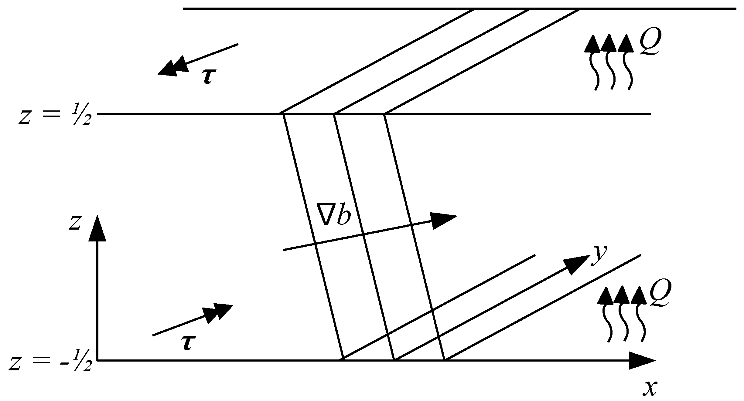
. Our nondimensional setup is shown in
Figure 2 for a typical isolated front.
Note that we have applied opposing wind stress and buoyancy flux to each surface due to the change in the direction of the surface normal vector. For stress-driven flow in a shallow sea, we might anticipate that the bottom stress will oppose the surface stress at a steady state. However, rather than representing any physical processes, our approach is primarily for mathematical convenience as it makes the problem vertically symmetric and eliminates any net translation of the front. We expect that having forcing at the top and bottom likely enhances the effect of the forcing by about a factor of two for a given forcing strength, relative to what would happen if the forcing was only applied to one boundary. A similar choice was made in the simulations of convection reported in Callies and Ferrari [
24].
3. Analytic Solution
We consider the limit of small Rossby number and aspect ratio,
, and assume that the Ekman number and Prandtl number are order 1. We now expand the fields,
and
b, in powers of
as
and expand Equations (1) and (2) in powers of
. We also use a multiple timescale approach to expand the time derivatives as
for fast timescale,
, intermediate timescale,
t, and slow timescale,
. We can now consider the resulting equations at each order in
. For simplicity we consider the case of constant
and
. Solutions can be found for
and
as general functions of
z (see [
1]). Depth-averaged quantities are written as
and departures from the depth-average are defined as
. We consider a vertical domain
so the depth average is defined as
The dimensionless heat flux is given by
and the dimensionless wind stress magnitude by
where
and
are the dimensional heat flux and wind stress magnitude respectively. Here
is the heat capacity,
is a reference density,
g is the gravitational acceleration, and
is the specific heat capacity. Using typical parameters of
,
,
,
,
, and
we find that
and
, and motivated by this, we let
and
.
3.1. O(1) Balance
The leading order buoyancy equation is
with boundary conditions
at
. Assuming that any transients acting on the fast timescale have decayed, the solution is
which is vertically homogeneous. The leading order vertical momentum equation is hydrostatic balance
and hence
The leading order horizontal momentum equation is
which, upon ignoring fast time transients and substituting for
, gives
with boundary conditions
at
. This system can be solved (see
Appendix A) to obtain the solution
where
describes the modification of the thermal wind velocity by vertical mixing and is defined in Equation (
A7). Note that
acts as a streamfunction for the depth-independent component of velocity, as in geostrophic balance. The first term in square brackets describes the stress-driven components of the velocity with components both parallel and perpendicular to the surface stress. The second term in square brackets describes the buoyancy-driven flow and also has components parallel and perpendicular to the direction of the buoyancy gradient. In the case of no wind stress,
, and no depth-independent flow,
, the cross-front and along front velocities are given respectively by
where we note that
reduces to the linear ‘thermal wind’ profile,
z, in the case of
[
1]. By mass conservation we can calculate the vertical velocity as
which reduces to
in the case where
is homogeneous.
3.2. Balance
The
buoyancy equation is
with boundary conditions
at
. We begin by assuming that the fast time transients have decayed and depth average Equation (
22) to get
Subtracting Equation (
24) from Equation (
22) gives an equation for
,
The depth-dependent horizontal velocity is
and hence Equation (
25) becomes
which can be integrated to give
Recall that
is a function of
as described in (
A7). The first term in
describes the stratification induced by the surface buoyancy flux, the second term represents changes in buoyancy induced by wind forcing, and the third term represents the stratification induced by the TTW circulation [
1].
4. The Evolution of the Depth-Averaged Buoyancy
In order to determine the evolution of the buoyancy valid to
we solve for the leading order component of the buoyancy field,
, and can then use this in Equation (
28) to find the
contribution. Following [
1] we derive an equation in terms of
only by depth averaging the buoyancy evolution equation and substituting for
and
. Depth averaging the full buoyancy equation (see Crowe and Taylor [
1]) gives
which to leading order,
, reduces to Equation (
24) and can be written using the depth-averaged velocity as
where the depth-averaged pressure acts as a stream function for the depth-averaged velocity. In order to determine the full evolution another equation is needed to determine
. In Crowe and Taylor [
25] we used a depth-averaged vorticity equation to close the system and obtain two coupled equations in
and
. Here we instead assume that we can neglect the Jacobian term,
. One justification for this would be to assume that the characteristic along-front (
y) length scales are large. In this case
does not depend on the intermediate timescale,
t and so we must look to the
evolution equation.
The
depth-averaged buoyancy equation is
where
is a streamfunction for the depth-averaged flow
. We note that
and by symmetry we can assume that
is zero to obtain an equation for the slow evolution of
Again, we assume that we can neglect the Jacobian term to obtain
Note that while we have neglected all Jacobian terms, we retain the
y derivatives in the flux term and the diffusion term of Equation (
33). This is to give as much generality as possible since there is a much wider class of problems for which we can neglect the Jacobian derivatives than for which we can neglect the along-front second order derivatives. For example, in the case of the radially symmetric front considered by Shakespeare [
26], the Jacobian terms would vanish. However, the along-front derivatives in the flux term and diffusion term would describe the frontal curvature which can have significant effects on the structure of the front [
26]. Similarly, in the case of a fully 3D system, baroclinic instability can generate modes with small along-front scales. For these small
y scales, the high number of derivatives in the flux term of Equation (
33) can cause it to dominate the Jacobian term and have significant effects on the formation of the instability [
25]. We will later neglect all
y dependence by assuming that any dependence on the along-front scale
y is weak due to along-front scales being much larger than cross-front scales. While this is a common approximation when studying frontal problems, it does prevent the growth of baroclinic instability [
25,
27]. The limitations of this approximation will be discussed in
Section 8.
Equation (
33) does not involve the
contribution to the horizontal velocity,
, and hence (
33) is a closed system involving
and known quantities. The term
can be written as
using the results for
and
. Depth-averaging this result gives
where the tensors
,
,
,
and
are defined in
Appendix B and are functions only of
. Note that
and
are fourth-rank tensors so here we use “·” to denote the contraction
. Substituting this result into Equation (
33) gives the evolution equation for the depth-averaged buoyancy,
Note that Equation (
36) is valid for
and
however, in the case of constant
and
the term
is constant and hence can be neglected.
Physically, the leading-order velocity perturbation consists of a TTW component, , plus an Ekman velocity driven by the wind stress, . Since the leading order velocity controls the vertical buoyancy gradient, , through an advection–diffusion balance, is determined by the advection of the background horizontal buoyancy gradient and the surface buoyancy flux. Therefore consists of three terms, corresponding to the stratification maintained by TTW flow, corresponding to the stratification maintained by the wind-driven Ekman flow and describing the buoyancy flux induced stratification.
From Equation (
33) we can see that the correlation between the stratified component of the buoyancy and the leading order velocity drives the evolution of the leading order buoyancy field via shear dispersion [
1]. This correlation term describes the horizontal flux of depth-averaged buoyancy and consists of six terms due to the advection of each of the stratification terms
,
and
by the velocity terms
and
. We therefore have terms proportional to
,
,
,
and
as shown in Equation (
36).
4.1. The y Independent Case
Our results can be simplified further if we neglect the remaining
y dependence from this point onward by assuming that any dependence on the along-front distance
y is small. In this case, Equation (
36) simplifies to
where
and the
are given in
Appendix B.
is linear in
and
,
consists of a part linear in
plus a part quadratic in
and
is linear in
. Note that
does not depend on the wind stress or buoyancy flux and hence is the same as in the unforced case [
1]. Spatial variations in the wind stress and buoyancy flux can cause the buoyancy field to evolve from an initially constant buoyancy through the
term which we anticipate could drive frontogenesis. Note that when any one coefficient is dominant we can find an approximate solution to Equation (
37) using the similarity solutions in
Appendix C.
For simplicity, we now reduce to the case where the wind stress,
, and buoyancy flux,
, are spatially uniform and hence constant. The limitations of this assumption are discussed in
Section 8. Equation (
37) becomes
and we write
where
describes the magnitude of the wind stress and
describes the angle from the positive cross-front direction in the right-handed sense. The coefficients,
,
and
can now be written as
and
using the results from
Appendix B. We now group the buoyancy flux term from
with
to write Equation (
39) as
where
and
Note that and are positive though and D may be negative.
4.2. Frontal Evolution
We now study the evolution of a simple
y independent front and find that wind stress and buoyancy flux may drive frontal spreading or sharpening depending on the parameter values. W begin by writing Equation (
44) as
where
If
is constant, then Equation (
48) reduces to the linear diffusion equation, although since
depends on the horizontal buoyancy gradient it will generally not be constant and Equation (
48) will be nonlinear.
It is difficult to obtain exact solutions to Equation (
48) due to the nonlinearity in
(implicit through
). In
Section 5, we will discuss numerical solutions to this equation. However, we can use insights from a linear diffusion equation with constant diffusivity to qualitatively predict the evolution of the front. In the linear diffusion equation, when
is a positive constant, the solutions will exhibit frontolysis through diffusive spreading. On the other hand, when
, the linear diffusion equation is ill-posed and solutions will exhibit sensitive dependence on the initial conditions and frontogenesis will occur through the development of step discontinuities in
.
Using the analogy of the linear diffusion equation we anticipate that frontolysis will occur when
for all
x. Note that the nonlinearity introduced through
and its dependence on
x mean that the behaviour is not guaranteed to hold. For example, Taylor and Zhou [
28] discussed a mechanism whereby steps can develop in a one-dimensional diffusion equation when the diffusivity depends on the buoyancy gradient. Nevertheless, our numerical solutions to Equation (
48) always exhibit spreading when
.
It is therefore of interest to determine the sign of
under various conditions, and this can be done by comparing the sizes of the terms in Equation (
48). If we assume that the front is oriented such that
then
can only be negative if
or
D are negative and sufficiently large compared to the other coefficients.
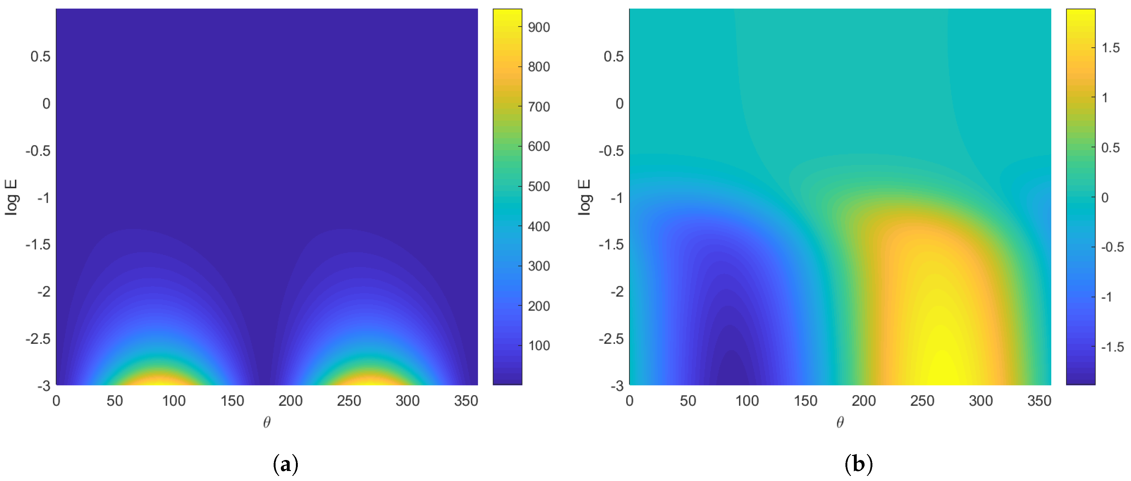
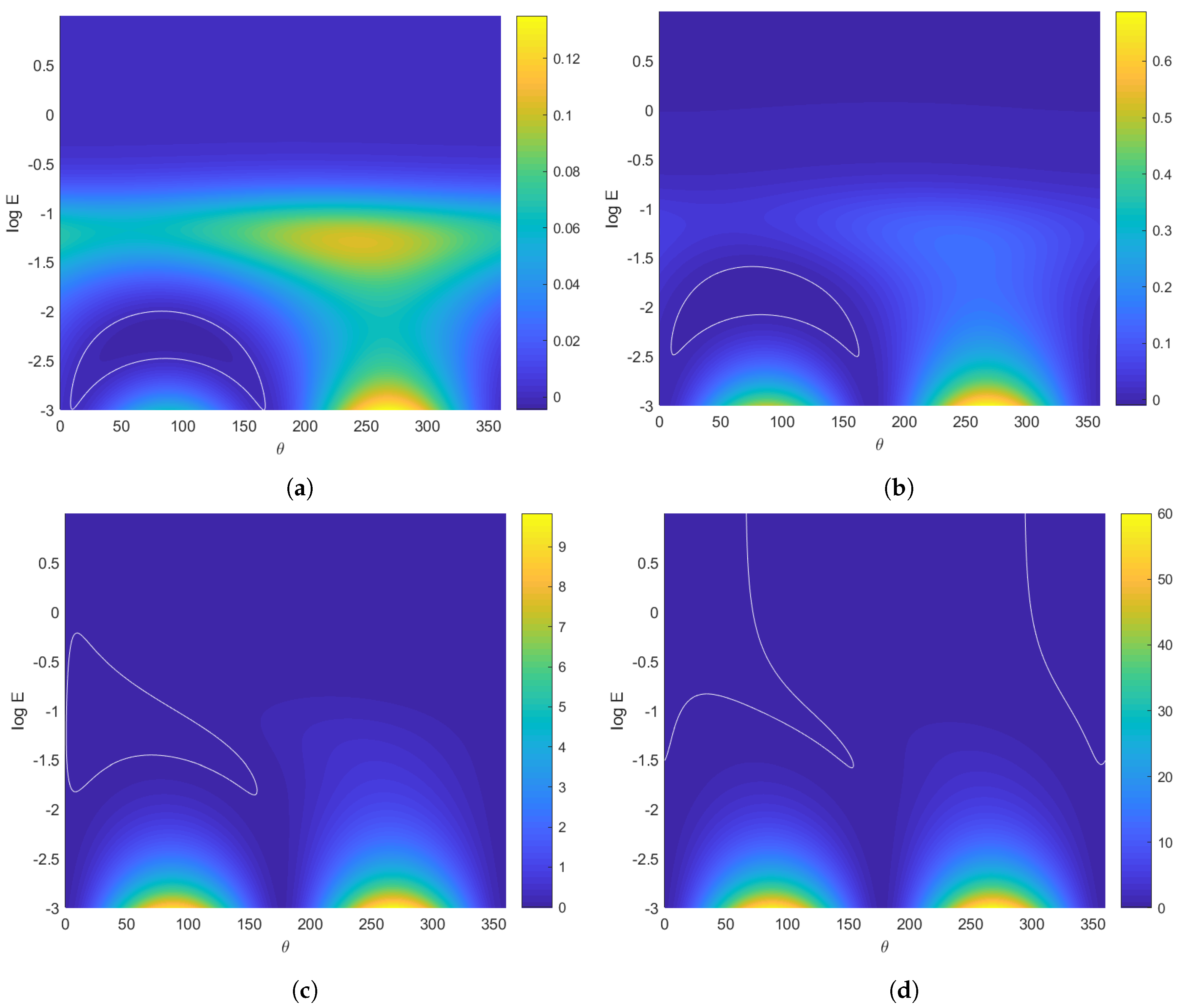
Figure 3 shows the coefficients
and
as functions of
and
. Recall that
is a positive function that is linearly proportional to the Ekman number. The coefficient
is positive for all values of
and
E while the largest amplitude negative values of
occur for small
E and
. Note that
,
and
for small
, hence for small Ekman number and
we expect the front to spread through diffusion since the
term will be dominant in that limit. For intermediate values of
it may be possible for a negative
or
D to temporarily sharpen the frontal gradients. However, since the front sharpens, the cubic term in Equation (
44) will become large and, since
, the gradient will not increase indefinitely.
From Equation (
49), we see that
when
where
assuming that these roots are real. Negative values of
occur when
and
is positive when
and
.
In many cases, we expect fronts to evolve towards an equilibrium state with a buoyancy gradient
. This follows if we first assume that
leads to the spreading of the front so that
decreases in time. If the buoyancy gradient
, then we anticipate that the buoyancy gradient will decrease until
where
and an equilibrium state is achieved. On the other hand, if
, existing fronts can intensify through reverse diffusion and
will increase until
. In both cases,
acts as an attracting equilibrium state.
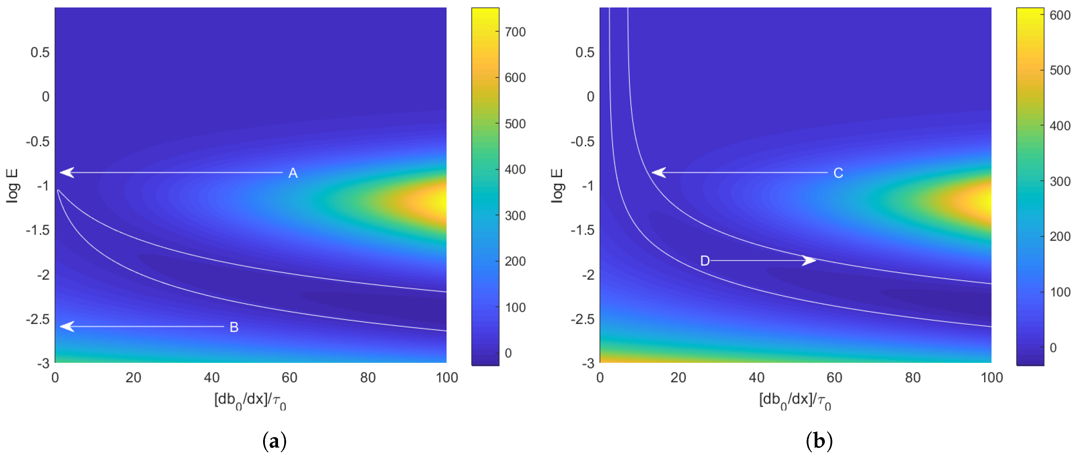
Figure 4, which is discussed below, illustrates this argument in the case of no surface heat flux.
To make this idea more precise, consider an initial non-dimensional buoyancy gradient, . If there are no positive real roots, then is initially positive and remains positive throughout the evolution, and we anticipate that the front will spread. If there are positive real roots then we have three possible cases. Firstly if then is initially positive and the front spreads indefinitely with increasing throughout the evolution. Secondly if then is initially negative and the front sharpens towards ; as this critical gradient is approached so the front will sharpen towards an equilibrium gradient. Finally if then initially so the front will spread towards and again approach an equilibrium width.
Consider a situation where
and the second term in Equation (
48) causes
. Physically, this can be interpreted as a wind-driven Ekman flow that opposes the cross-front TTW flow in such a way that the overall buoyancy flux is reversed, resulting in an up-gradient flux. Similarly, when
(the diffusivity associated with the last term in Equation (
44)) and the surface cooling is sufficiently strong to create regions of unstable stratification also leads to an up-gradient flux of buoyancy.
Note that it is possible for density inversions to occur in cases where the wind stress opposes the cross-front TTW flow or when the buoyancy flux is negative. Theoretical studies by Thomas and Rhines [
29] and Benthuysen and Thomas [
30] using diffusive parametrisations have also noted these inversions. Below we will consider two limits where the solutions can be simplified, specifically the limits of a weak surface heat flux and a weak wind stress.
4.3. Weak Surface Heat Flux
We begin by considering the case of a weak surface heat flux (and small
D in Equation (
44)) where the effects of buoyancy flux and horizontal diffusion can be neglected.
Figure 5 shows
as a function of
and
(the base 10 logarithm is used for the figures throughout) for
and
. Panels (a)–(d) correspond to four different values of the wind stress,
and the white contour marks
. The size and shape of the region where
is strongly dependent on
. For a particular Ekman number,
typically occurs for a limited range of wind stress orientations. This is a consequence of the coupling between the along-front and cross-front velocities through the vertical mixing and rotation terms. When the wind stress is weak (and
is small), the largest negative value of
occurs for small Ekman number and when
, i.e., when the wind stress is aligned with the thermal wind in a down-front orientation. In this orientation, the cross-front Ekman transport acts to advect water from the dense side of the front over the top of the water from the light side of the front [
10].
Conversely, when the wind stress is strong, the largest negative value of occurs for large Ekman numbers. In this limit when vertical mixing is strong, the flow is more closely aligned with the wind stress and the strongest cross-front flow occurs when the wind is closer to the cross-front direction. As a result, the largest negative value of occurs for smaller values of , when the wind stress is more closely aligned with the buoyancy gradient.
For
, the diffusivity,
, can be written
Note that the sign of
is a function only of three parameters;
,
and
.
Figure 5 shows
as a function of
for
and
= 45°,
°. These values of
were chosen due to having regions of both positive and negative
. For the purpose of discussion, points A–D correspond to particular initial conditions. For cases starting at points A and B,
initially, and the front will spread such that
as indicated by the arrows. If
E is constant, we anticipate that the fronts in these cases will spread indefinitely since
never reaches zero. In case C
initially. However, as
decreases for a constant
E,
will reach zero at an equilibrium buoyancy gradient. Case D has
initially and we anticipate buoyancy gradients to sharpen until
.
Following the thought experiment described above, we might anticipate that fronts will evolve until they reach a state of equilibrium where
. The equilibrium buoyancy gradient can be found by setting
in Equation (
52) and solving for
. The equilibrium value of
, denoted
can then be written
Note that the equilibrium gradient is proportional to the wind stress, so stronger wind stress will sustain a stronger equilibrium gradient.
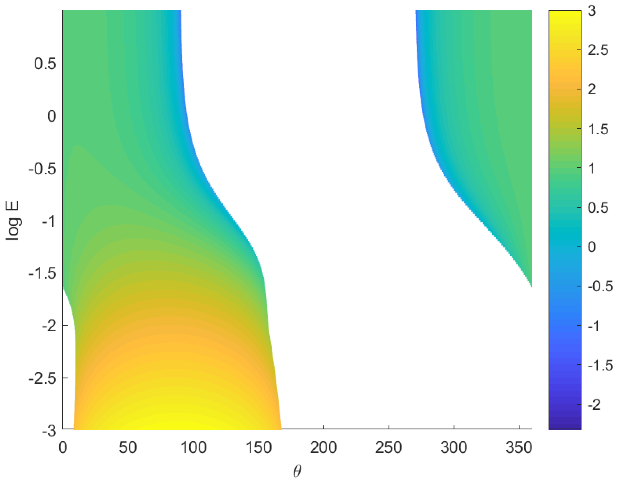
Figure 6 shows
as a function of
and
. The white region corresponds to the range of parameters where an equilibrium buoyancy gradient does not exist. Note that the equilibrium buoyancy gradient decreases with increasing Ekman number. This suggests that vertical mixing counteracts wind-driven frontogenesis and that this balance holds for weaker buoyancy gradients when mixing is strong.
4.4. Weak Wind Stress
For small
, the evolution of the leading order buoyancy, Equation (
44), reduces to
This is the nonlinear Erdogan–Chatwin equation [
31,
32] discussed in [
1] with the horizontal diffusivity,
, replaced by the combined diffusivity,
. The surface buoyancy flux modifies the coefficient of the linear diffusion term and hence increases the spreading rate in the case of surface heating and reduces the spreading rate for surface cooling.
When
D is positive
is strictly positive and is given by
In this case, Equation (
54) can be solved using similarity solutions and describes a spreading front [
1,
32]. Furthermore, if
D is large compared with
, Equation (
54) reduces to a linear diffusion equation with the similarity solution
Over long times, the linear terms in Equation (
54) dominate the nonlinear term and the front spreads as
and approaches this similarity solution.
If
D is negative, corresponding to surface cooling that is sufficiently strong to overcome the spreading effects of horizontal diffusion, we may write
so
may be written as a function of
as
where we recall that
Therefore, there will always exist a region where
and we have equilibrium buoyancy gradient (where
) of
In this case we have
so, as discussed above (in the text below Equation (
51)), we do not anticipate indefinite frontolysis. Instead, we expect that the front will either spread (
) or sharpen (
) until
reaches the equilibrium value,
.
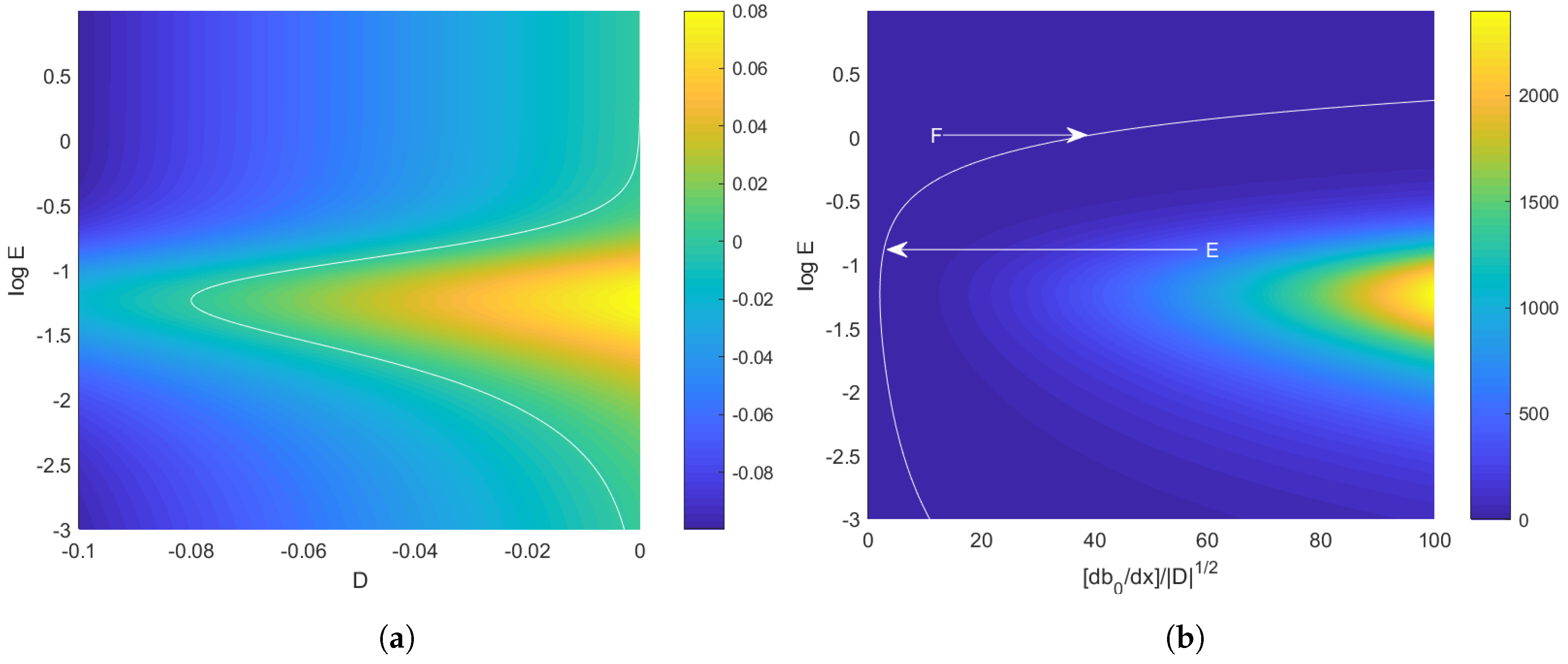
Figure 7a shows
as a function of negative
D and
for
and
. The region where
occurs to the left of the white line.
Figure 7b shows
as a function of
and
for
and
. Again the white contour denotes
and hence corresponds to the equilibrium gradient
. Similarly to
Figure 5, point E corresponds to a front spreading towards equilibrium whereas point F corresponds to a front sharpening towards equilibrium.
5. Numerical Simulations
In this section, we describe numerical solutions of the evolution equation for the leading order buoyancy, Equation (
44). The objective of these simulations is to test our predictions about frontal spreading or sharpening based on the sign of
and to examine the behavior in more detail. We use a pseudo-spectral method to evaluate the spatial derivatives and a fourth-order Runge-Kutta scheme for the time stepping. We assume that the leading order buoyancy,
, is a function of
x and
t and we use a spatial grid with
grid points.
We use a numerical domain of nondimensional width
with
and an initial buoyancy profile of
so
Note that the horizontal lengthscale
L used to nondimensionalise
has been arbitrary up to this point; setting
in the center of the front is equivalent to choosing
L to be the frontal width
so is not an assumption which imposes any restrictions on our method. In order to make the domain periodic and use a pseudo-spectral method we subtract a linear profile from
and solve for
where
We now present three different cases of sharpening and spreading fronts that can arise from different choices of parameters.
Figure 4 is used to help select the parameters for the different cases.
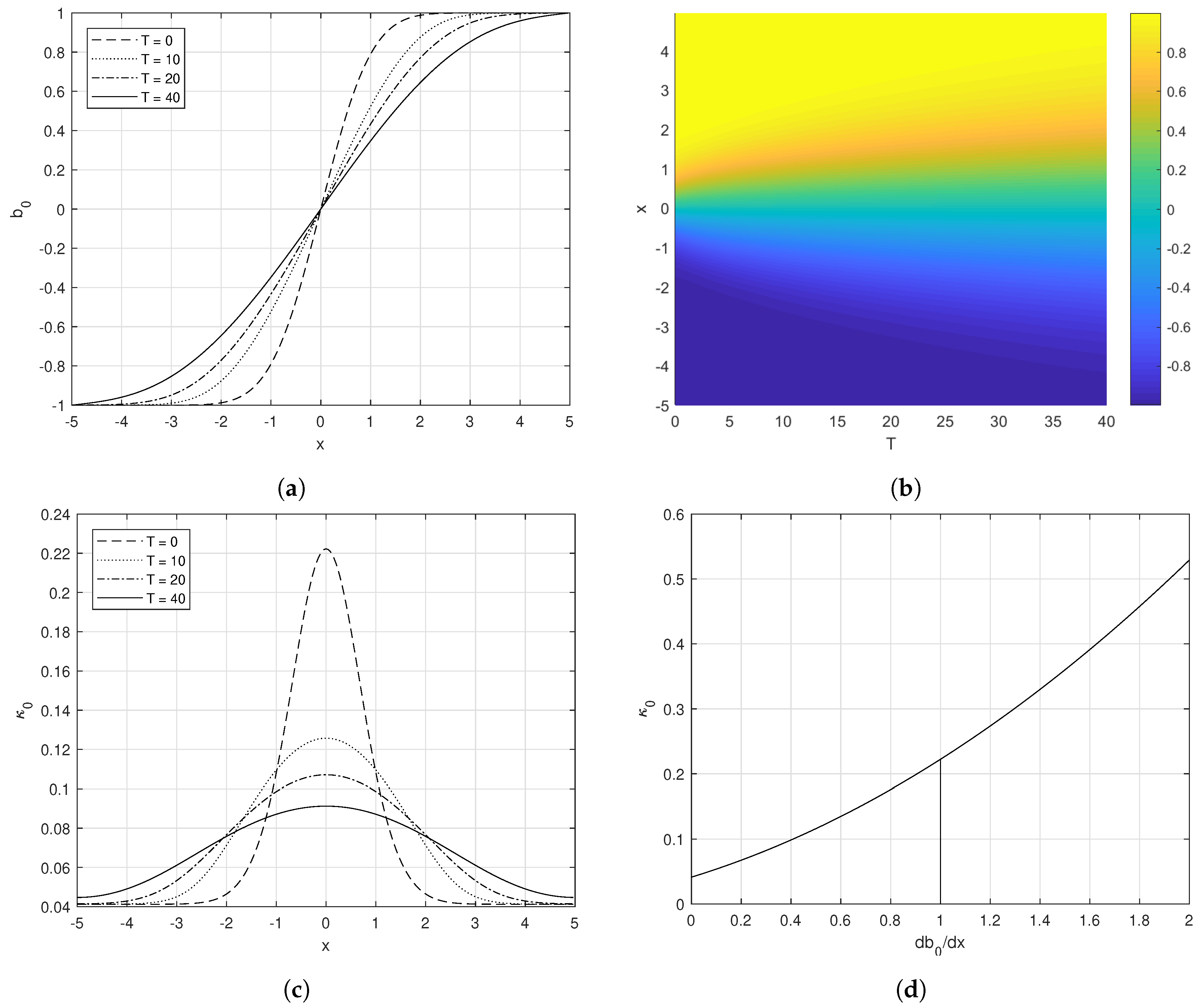
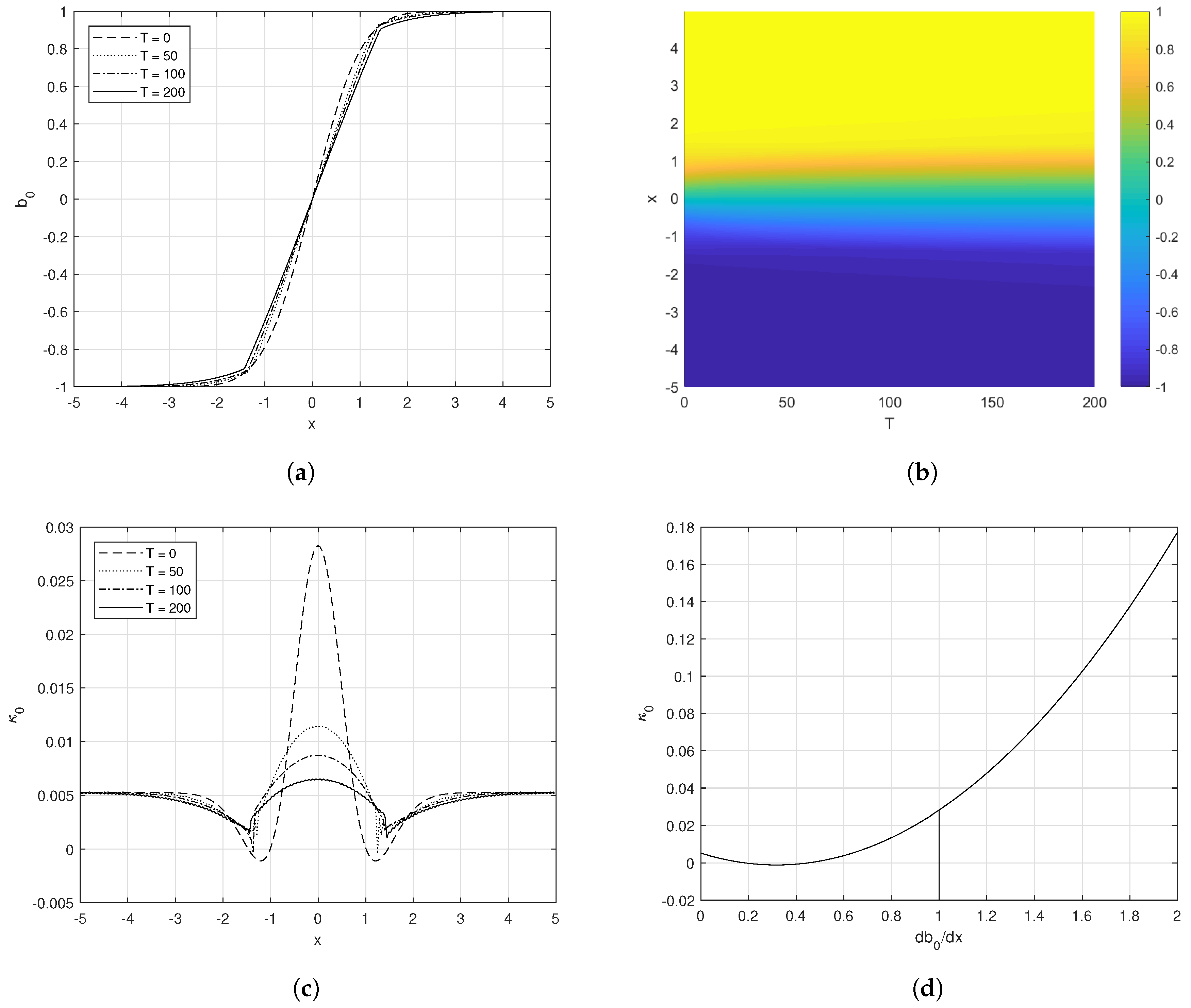
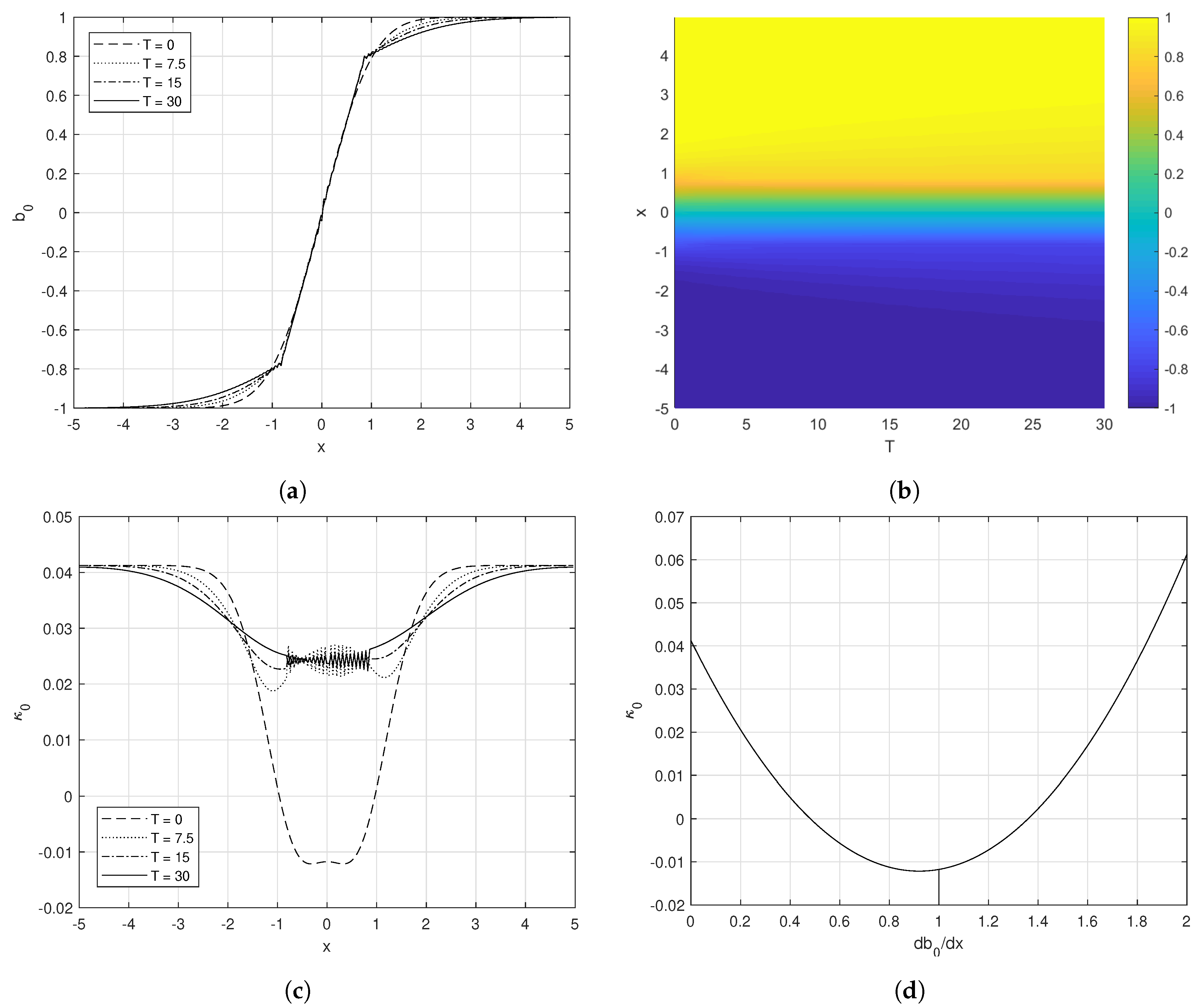
For each simulation, we plot as a function of x and T showing any spreading, as functions of x for several values of T showing the shape of the cross-front buoyancy profile, as a function of x for several T values to show the cross-front variation in spreading rate, and as a function of to see how the spreading rate changes as the front evolves and if there exists an equilibrium buoyancy gradient, .
5.1. A Spreading Front—Indefinite Spreading
We begin by considering a case where there is no real positive equilibrium gradient,
. This case has a surface wind stress partially opposing the thermal wind and no surface heat flux. Specifically, the parameters are
,
,
°,
,
and
. The corresponding coefficients are
,
,
and
. The numerical solution is shown in
Figure 8. The horizontal diffusivity can be much different inside the front than it is towards the edges due to the dependence of
on
. In this case,
is larger inside the front than at the edges, leading to an approximately linear cross-front buoyancy profile near
. We note that it is possible to have cases with
where
is smaller inside the front than at the edges.
Qualitatively similar behavior also occurs in the absence of wind stress and a small or zero heat flux. When both the wind stress and the surface heat flux are zero, the solution limits to that described in [
1]. In these cases the cubic nonlinear term in Equation (
44) is dominant inside the front and the solution resembles the similarity solution,
(see
Appendix C).
5.2. A Spreading Front—Equilibrium Width
We now consider the case where there exists a real, positive equilibrium gradient with
. Specifically, consider a wind oriented
away from the cross-front direction in the absence of a surface heat flux with parameters
,
,
°,
,
and
. The corresponding coefficients are
,
,
and
and the numerical solution is shown in
Figure 9. Near
the front spreads towards a constant gradient. Initially, there are regions in which
, where the gradient sharpens to match that of the interior region, forming cusps between the spreading edges and the approximately linear interior profile. Once the cross-front buoyancy profile reaches the equilibrium gradient,
, we expect it to remain constant in time near
.
5.3. Sharpening Front
Finally, we consider the case of a real, positive equilibrium buoyancy gradient with
with parameters
,
,
°,
,
and
. The corresponding coefficients are
,
,
and
and the numerical solution is shown in
Figure 10. At the centre of the front,
initially, and the cross-front buoyancy profile sharpens into a series of steps. Towards the edges of the front
and the front spreads.
We note that due to the ill-posed nature of backwards diffusion, numerical solutions of Equation (
44) with
in some regions will not be accurate. In particular, spikes in the buoyancy gradient start to develop, and increasing the grid resolution will only result in more small-scale oscillations as energy is transferred into the highest frequency modes. However, we expect that the qualitative behaviour will be similar to that observed here with a sharpened frontal region and spreading edges.
7. Equilibrium Width Due to Stress-Ekman Balance
In this section, we discuss the scaling for the dimensional equilibrium horizontal buoyancy gradient and the implications for typical frontal widths. As discussed in the introduction, these results have implications for parameterisations of submesoscale processes which typically require the horizontal buoyancy gradient as a parameter (e.g., [
19,
33]).
The expression for the equilibrium horizontal buoyancy gradient given in Equation (
53) can be written in terms of dimensional variables,
where
and
Here
describes the strength of the combined horizontal diffusivity due to horizontal mixing and the surface heat flux compared with the strength of the diffusivity associated with the wind stress. We expect this ratio to be small as explained in
Section 6.2.
For illustration, consider a simple case where
and
= 90°, i.e., no explicit horizontal diffusion in the buoyancy equation, no surface heat flux, and a wind stress aligned with the horizontal buoyancy gradient (cross-front wind stress). In this case the coefficients in Equation (
48) are
and hence the function in Equation (
73) reduces to
and therefore the dimensional equilibrium buoyancy gradient is
since
for turbulent diffusivity
. The value for
(and hence
) may be taken from observations or estimated via Equation (
64) or Equation (
66) for the cases of surface wind stress driven turbulence or surface cooling driven turbulence respectively. Typical values, e.g.,
,
and
give an equilibrium buoyancy gradient of
This value is well-within the typical range for submesoscale fronts in the open ocean (e.g., [
34]). For these parameters that are typical of submesoscale fronts, using our definition, the Rossby number in this case is
using a horizontal lengthscale of
km and
. Therefore, our analysis for the equilibrium frontal width can still apply to submesoscale fronts in a parameter range where
is small enough for our asymptotic analysis to be valid. However, for weaker mixing or stronger wind stress, the sharpening effects of the wind stress dominate over the buoyancy-driven spreading and the front sharpens towards an equilibrium state with a larger Rossby number where our model equations might break down.
Jindasa et al. [
35] found that frontogenesis can sharpen a submesoscale front to scales of only a few meters, in this case, large Rossby number effects dominate rotation and the front behaves like a gravity current. While our model is not valid for large Rossby numbers, it is possible that the mechanism of frontal sharpening due to the coupling of turbulent mixing and wind stress described here can act to sharpen fronts to a point where finite Rossby number effects take over. Therefore our analysis may provide a framework for examining when extreme sharpening can happen.
Note that an equilibrium frontal width will only exist if the Ekman flow opposes the cross-front TTW flow. If the TTW flow is initially stronger (i.e., the initial buoyancy gradient is stronger than the equilibrium buoyancy gradient), then the front will spread towards an equilibrium, whereas if the wind stress-driven flow is stronger, the front will sharpen towards an equilibrium. In the latter case, sharpening may lead to small regions of sharp buoyancy gradient resulting in a step-like series of small fronts, rather than a narrowing of the whole frontal region.
8. Conclusions and Discussion
We have considered an analytical model of a mixed layer front forced by surface fluxes of buoyancy and momentum. Using an asymptotic expansion in the Rossby number we determined the leading-order velocity and buoyancy perturbations. By calculating the depth-averaged buoyancy fluxes, we then showed that the leading order buoyancy satisfies a nonlinear diffusion equation where the diffusivity depends on the surface-forcing and the strength of the mixed layer turbulence.
Depending on the direction of alignment between the front and the wind stress we found that it is possible for the front to sharpen or to spread. Sharpening occurs when the wind stress drives a cross-front flux that opposes and overcomes the TTW-driven cross-front flux and leads to a horizontal convergence in the buoyancy field. Spreading occurs when the stress-driven flux either reinforces the TTW flux or opposes but does not exceed it and the front then spreads via shear dispersion [
1,
21,
36].
We find that surface heating can also act to spread the front due to the upward advection of less buoyancy fluid by the vertical velocity. Surface cooling may lead to frontal sharpening if it is sufficiently strong to overcome the spreading effect of horizontal mixing. Additionally, surface cooling may act to enhance the mixed layer turbulence which will lead to a faster horizontal spreading via shear dispersion due to an increased Ekman number [
1].
Note that since we used a diffusive parametrisation for mixed layer turbulence and did not consider the effects of gravitational instability or convective overturning, our model can develop a gravitationally unstable density profile in the cases of surface cooling or strong wind stress opposing the cross-front TTW velocity. These inversions have been noted in previous theoretical studies [
29,
30], although modelling studies have found that symmetric instability is effective at re-stratifying the mixed layer beneath a ‘convective layer’ [
4]. We have not considered the influence of symmetric instability (or other submesoscale instabilities) here.
For intensifying fronts, we find that the increase in the horizontal buoyancy gradient increases the frontolytic tendency of the cross-front TTW velocity. Eventually, this balances the frontogenetic tendency associated with surface-forcing, and the front approaches a balanced state with an equilibrium buoyancy gradient. Similarly, fronts may spread towards an equilibrium width if the frontolytic effect of the cross-front TTW velocity is stronger than the frontogenetic effect of the surface forcing. Due to the nature of backward diffusion, any sharpening will likely form small steps in the buoyancy profile rather than a significant narrowing of the frontal region.
The equilibrium state that we find from the asymptotic theory and numerical solutions when frontogenesis associated with the surface-forcing is balanced by spreading associated with the TTW circulation, may provide a means of maintaining a particular frontal width. Additionally, when surface-forcing induces frontolysis, this effect could act to counteract frontogenesis associated with other processes such as an external strain flow or the TTW secondary circulation [
8,
17].
Using typical parameters for ocean fronts we have estimated values for the equilibrium buoyancy gradient. Our prediction is of a similar magnitude to the gradients observed in strong submesoscale fronts and much stronger than the buoyancy gradients predicted by global ocean models due to these models not fully resolving submesoscale features. Therefore, our predictions for the scaling of the equilibrium buoyancy gradient may be useful for parametrising the frontal strength in models that do not resolve these scales.
Throughout our analysis, we have made several simplifying assumptions. Some of these can be easily relaxed, while others impose limitations on our method. Firstly, we have assumed that the turbulent viscosity and diffusivity are constant in both space and time. It is possible to use depth-dependent profiles for
and
using the approach given in Crowe and Taylor [
1]. This would not qualitatively influence solution beyond modifying the coefficients,
. Physically, we might also expect cross-front and time variations in
and
due to the large-scale properties of the front [
4,
37]. However, the extent of these variations or their influence on frontal dynamics remains unclear. Time-varying viscosity and diffusivity may lead to feedback between the frontal evolution and the turbulent mixing which would change the time-dependence of the solution.
Secondly, several approximations have been made regarding the surface-forcing. In particular, we have assumed that the forcing is spatially independent and applied to both top and bottom surfaces. The application of forcing to both the top and bottom boundaries was discussed at the end of
Section 2 and more realistic forcing will likely give similar results. While spatial dependence of the forcing has been neglected throughout, it could be easily introduced since Equation (
36) can be used with a spatially varying
and
. We expect this to lead to complicated dynamics in which different regions of the front evolve differently, potentially leading to along-front (
y) variations.
Finally, we have assumed a scale-separation between the along-front and cross-front scales. While this assumption is valid for most observed fronts, it does prevent the formation of baroclinic instability, which we showed was significantly modified by vertical mixing in [
25]. Baroclinic instability may act to modify small-scale turbulence (e.g., [
37]) or stratification (e.g., [
33]), which could, in turn, modify the dynamics considered here.
