A Numerical Study of Metachronal Propulsion at Low to Intermediate Reynolds Numbers

Abstract

Inspired by the forward swimming of long-tailed crustaceans, we study an underwater propulsion mechanism for a swimming body with multiple rigid paddles attached underneath undergoing cycles of power and return strokes with a constant phase-difference between neighboring paddles, a phenomenon known as metachronal propulsion. To study how inter-paddle phase-difference affects flux production, we develop a computational fluid dynamics model and a numerical algorithm based on the immersed boundary method, which allows us to simulate metachronal propulsion at Reynolds numbers (RE) ranging from close to 0 to about 100. Our main finding is that the highest average flux is generated when nearest-neighbor paddles maintain an approximate 20%–25% phase-difference with the more posterior paddle leading the cycle; this result is independent of stroke frequency across the full range of RE considered here. We also find that the optimal paddle spacing and the number of paddles depend on RE; we see a qualitative transition in the dynamics of flow generated by metachronal propulsion as RE rises above 80. Roughly speaking, in terms of average flux generation, a tight paddle spacing is preferred when RE is less than 10, but a wider spacing becomes clearly favored when RE is close to or above 100. In terms of efficiency of flux generation, at RE 0.1 the maximum efficiency occurs at two paddles, and the efficiency decreases as the number of paddles increases. At RE 100 the efficiency increases as the number of paddles increases, and it appears to saturate by eight paddles, whereas using four paddles is a good tradeoff for both low and intermediate RE.

1. Introduction

Long-tailed crustaceans, including crayfish, krill, prawns and lobsters, swim forward by beating four or five pairs of limbs called swimmerets rhythmically through cycles of power-strokes (PS) and return-strokes (RS) (see Figure 1) [1]. While the two limbs within each bilateral (left–right) pair move in phase relative to each other, nearest-neighbor limbs in each ipsilateral (anterior–posterior) pair move with a metachronal rhythm: movements of the posterior and anterior limbs maintain a nonzero phase-difference. Despite the large variation of stroke frequency, movements of the ipsilateral limbs maintain an approximate quarter-period phase-difference, independent of the stroke frequency, with the more posterior limbs leading the cycle [2].

It is believed that this tail-to-head (or back-to-front) propagating metachronal wave in limb beating provides a significant fluid dynamics advantage compared to other stroke patterns [3,4,5]. Using mechanical models based on drag forces, Williams [6] and Alben et al. [7] argued that the metachronal rhythm contributed to a smoother body velocity time course. In addition, Alben et al. examined how inter-limb phase-difference influences average body velocity and predicted that metachronal rhythms led to a slightly higher (less than 10%) average body velocity compared to the in-phase (synchronous) rhythm. However, drag-force-based models cannot distinguish the direction of metachronal waves, i.e., the tail-to-head metachronal rhythm with a 25%-period inter-paddle phase-difference (with the more posterior paddle leading the cycle) cannot be distinguished from the head-to-tail metachronal rhythm with a 75%-period phase-difference (with the more anterior paddle leading the cycle). Furthermore, drag-force-based models cannot capture fluid-structure interactions between the paddles, the effect of which can be too significant to ignore especially for tightly spaced paddles.

In a recent work [8] by some of the authors of this article, Zhang et al. constructed a two-dimensional fluid dynamics model of crustacean swimming, which consisted of a fixed wall with four rigid paddles attached underneath that moved in various prescribed metachronal rhythms. To mimic the asymmetry between the straight limbs during PS and the curled limbs during RS in crustacean swimming, the authors modeled the limbs as nonporous paddles during PS and porous paddles during RS. The natural variation in swimmer size and stroke frequency leads to Reynolds numbers (RE) ranging from about 10 to 1000, in which both viscous and inertial effects are relevant. Under this setting, they found that, over RE ranging from 50 to 800, the tail-to-head metachronal rhythm with an approximate 25% inter-paddle phase-differences led to a 60% increase in average flux compared to the in-phase rhythm and a 500% increase compared to the head-to-tail metachronal rhythm. They also used a simple geometric argument to illustrate that the asymmetric, 25%-period delayed arrangement of neighboring limbs during PS and RS creates an advantage by enclosing a larger volume of fluids underneath the paddles during PS and trapping a smaller volume of fluids during RS (see Figure 4 in [8]).

More recently using particle image velocimetry measurements on a robotic model, Ford et al. investigated metachronal paddling in the RE range from 50 to 800 [9]. They found that metachronal paddling produced significantly more vertical movement of fluid compared to in-phase (synchronous) paddling at higher RE. This vertical flow is important for generating lift. Metachronal paddling at low RE have been investigated both theoretically [10] and experimentally [11] by Takagi. Their theory predicts that the direction of locomotion is in the same direction as the metachronal wave, which is consistent with crustacean locomotion at higher RE.

Thus metachronal propulsion is effective for locomotion across a range of scales ranging from the small scale where inertia is negligible to larger scales where vortex interactions are significant. However, previous studies have not addressed how the fluid dynamics of metachronal paddling change qualitatively as the RE ranges from 0.1, where inertia is negligible, to 100, where vortex dynamics becomes significant. It is not clear if the fluid dynamical advantage of the approximate 25% phase-difference in metachronal paddling reported in [8] would persist as the RE decreases from 50 to 0. In this work, we examine metachronal propulsion specifically in the RE range from 0.1 to 100, and we explore how the optimal phase difference, paddle spacing, and number of paddles vary with RE in this range. We assume that the power-stroke and return-stroke are mirror images of each other; i.e., there is no drag asymmetry in the paddling direction. Note that in [8] a “porous” paddle was used for return-strokes to account for a reduction in drag during the return-stroke phase of paddling; this was an extra asymmetry in the paddling kinematics in addition to the asymmetry in the direction of the metachronal wave. Here, however, we implement a simple, symmetric power and return stroke to remove confounding factors from the modeling parameters of our greatest interest: the phase-difference between neighboring paddles, paddle spacing, and the number of paddles. Thus the only asymmetry in the swimmer model considered in this work comes from the phase differences of the metachronal wave of motion of the paddles. We perform a systematic numerical study to investigate the effects of phase-difference, paddle spacing, and the number of paddles on metachronal propulsion over the RE range of 0.1–100.

2. Model Formulation

Our model consists of n rigid, equal length paddles moving with prescribed motion attached to a fixed horizontal wall (mimicking the body) immersed in a two-dimensional fluid. The paddles are indexed $i=1,\dots ,n$ from left to right. The motion of the ith paddle is prescribed by its angle, ${\alpha }_i$, formed from the wall (body) to the paddle, and is given by

$${\alpha }_i\left(t\right)=\overline{\alpha }-Acos\left(2\pi \left(\frac{t}{T}+{\varphi }_i\right)\right),$$

(1)

in which $A=\pi /4$ is the amplitude, $\overline{\alpha }=\pi /2$ is the mean angle, t is the time, T is the period of stroke, and ${\varphi }_i$ is the phase of paddle. Note that the cyclic movements of the four or five pairs of limbs in long-tailed crustaceans share roughly the same period, and therefore we define the time it takes for a single limb to complete a full cycle of power and return stroke as one period of stroke. The paddles are of uniform length, ℓ, and are equally spaced along with wall, separated by distance w at the base. See Figure 2 for an illustration of our model.

We note that in this model the motion of a single paddle is symmetric in both time and in the horizontal direction; i.e., power-stroke (PS) and return-stroke (RS) are exact mirror images of themselves. A single paddle would produce no net motion of the fluid. The only asymmetry in our n-paddle swimmer model ($n\ge 2$) arises from the inter-paddle phase-difference $\Delta \varphi$ between neighboring paddles.

We consider constant phase differences between neighboring paddles: $\Delta \varphi ={\varphi }_{i+1}-{\varphi }_i$ for all i, in which $-0.5<\Delta \varphi \le 0.5$. When all paddles beat in-phase (synchronously) $\Delta \varphi =0$, and when adjacent paddles beat in antiphase $\Delta \varphi =0.5$. For other values of $\Delta \varphi$ the paddling motion is a metachronal wave. We consider a rightward (in the head-to-tail direction) moving paddle as moving in the positive direction because it moves fluid to the right. For $0<\Delta \varphi <0.5$, the motion of the paddles is a leftward (tail-to-head, or back-to-front) moving wave of positive paddling, and for $-0.5<\Delta \varphi <0$, the motion is a rightward (head-to-tail, or front-to-back) moving wave of paddling.

The motion of the paddles drives the motion of the surrounding fluid. The equations that determine the motion of the fluid are the incompressible Navier–Stokes equations:

$$\begin{array}{c}\rho \left(\frac{\partial \mathbf{u}}{\partial t}+\mathbf{u}·\nabla \mathbf{u}\right)=-\nabla p+\mu \Delta \mathbf{u}+\mathbf{f},\end{array}$$

(2)

$$\begin{array}{c}\nabla ·\mathbf{u}=0,\end{array}$$

(3)

in which $\mathbf{u}$ is the velocity, p is the pressure, $\mu$ is the viscosity of water, $\rho$ is the density, and $\mathbf{f}$ is the applied force density which arises from the prescribed motion of the paddles.

The domain is taken to be a channel of height 1 (i.e., length is scaled by the channel height) with no slip boundary conditions at the top and bottom and periodic boundary conditions in the horizontal direction. Different length channels are considered for different experiments as described in the results section. The period of stroke is taken to be 1 (i.e., the time is scaled by the period), and thus the velocity scale of the computation is the channel height divided by the period. The paddle length is taken to be $0.15$ times the channel height to be consistent with [8].

The Reynolds number (RE) is defined using the paddle length, ℓ, as the characteristic length, and the maximum speed of the paddle tip, $U_{\max }=2\pi A\ell /T$, as the characteristic velocity:

$$\mathrm{RE}=\frac{2\pi A{\ell }^2\rho }{\mu T}.$$

(4)

Note that the length and velocity scales for the computation are distinct from those used to define the RE.

In this study we explore how the paddle spacing, the inter-paddle phase-difference, and the RE affect the paddling performance, which we quantify by the time average of the flux (amount of fluid per unit time) through the channel. The flux is

$$Q\left(t\right)={\int }_0^1\mathbf{u}·\widehat{\mathbf{x}}dy,$$

(5)

in which $\widehat{\mathbf{x}}$ is the unit vector pointing in the horizontal direction. The time-averaged flux is

$$\langle Q\rangle ={\int }_{t^{\prime }}^{t^{\prime }+1}Q\left(t\right)dt,$$

(6)

in which the flux is averaged over one period (the period is 1) from some time $t^{\prime }$ to $t^{\prime }+1$. Note that Q (and thus $\langle Q\rangle$) is independent of x because the flow is incompressible.

For details about the numerical method, see Appendix A.

3. Results

Using the two-dimensional paddling model described in the previous section, we simulate numerically the fluid motion arising from various prescribed metachronal paddling rhythms under a range of Reynolds numbers (RE) from 0.1 to 100. We focus on three model parameters that determine the paddling rhythm: the phase-difference between neighboring paddles ($\Delta \varphi$), paddle spacing (w), and the number of paddles (n). When we vary one model parameter, we keep the remaining parameters constant. Unless otherwise stated, we perform each simulation for 10 periods of strokes. We measure the performance of each paddling rhythm by the average flux production $\langle Q\rangle$ (defined in Equation (6)), except when we investigate the effect of the number of paddles on swimming, we use the efficiency of average flux generation as our measure (defined in Section 3.5).

We first show that the highest average flux is achieved when $\Delta \varphi \approx$ 20%–25% (with $w=0.375$ and $n=4$) under all four values of RE considered ($\mathrm{RE}=0.1$, 1, 10, and 100). We then explore how paddle spacing w affects the average flux (with $\Delta \varphi =25$% and $n=4$). While the optimal phase-difference is insensitive to changes in RE, the optimal paddle spacing depends on RE. This leads us to explore the changes in flow structure as RE increases. Roughly speaking, we observe a qualitative transition in the fluid dynamics of metachronal propulsion at RE $\approx 80$. We find that a tight paddle spacing ($w\approx 0.2$) is preferred at small RE (less than 80), and a wide spacing ($w\approx 0.4$) becomes desirable at higher RE (greater than 80) during the start-up phase of paddling, while on longer time scales a tight spacing can also be effective. Finally, we investigate the optimal number of paddles n (with $\Delta \varphi =25$% and $w=0.375$) for swimming efficiency, a measure we define as the ratio of average flux production over average power consumption. We find that using about four paddles is a sweet spot for metachronal propulsion that provides a good trade-off under both low and intermediate RE (i.e., RE = 0.1 and 100).

3.1. The Effect of Phase-Difference on Flux

In our previous work [8], we used a similar model to understand how the phase-differences between neighboring paddles affected the average flux generation in a model swimmer with four paddles in the RE range of 50–800. In [8] we showed that an inter-paddle phase-difference around 20%–25% produced the highest average flux, independent of RE. Here we extend the previous study to lower RE in the range from 0.1 to 100. We use a domain of length 6 (same as that in [8]). There are four equally spaced (by 0.375 or 2.5 times their length) paddles that move with a constant phase-difference between adjacent paddles. The fluid starts at rest, and we compute the time-averaged flux over the 10th period.

The time-averaged flux as a function of the inter-paddle phase-difference is shown in Figure 3 for RE $0.1$, 1, 10, and 100. The fluxes are normalized by their maximum value for each RE. These results show that the peak flux occurs at around 20%–25% phase-difference between neighboring paddles for all RE. This result agrees with those presented in [8] for higher RE numbers.

Besides examining a different range of RE, there is one notable difference between the model used here and that used in [8]. Here the motion of each paddle is symmetric. There is no difference in the kinematics of the forward and backward stroke. In [8], the paddle was assumed permeable on the backward stroke resulting in a drag asymmetry to account for a difference in the drag on the power and return strokes in crustaceans. As expected, this symmetry results in zero net flux for $\Delta \varphi =0$ and $\Delta \varphi =\pm 0.5$, and similarly, the flux is an odd function of the phase differences. Because of the symmetric stroke of each individual paddle, the resulting nonzero fluxes are the result of the phase differences between paddles alone.

3.2. The Effect of Paddle Spacing

We now consider how the paddle spacing affects paddling performance for a fixed phase difference at different RE. The phase difference is fixed at 25% (which corresponds to the near peak flux) and the paddling spacing is varied between $0.175$ and $0.6$. The RE is again varied over the range from 0.1 to 100. The domain length is set to 3 to increase computational efficiency. A limited set of simulations were performed on a longer domain, and the results did not change qualitatively from the shorter domain.

Figure 4 shows the average flux, calculated over the 10th period of stroke, as a function of paddle spacing for RE $0.1$, 1, 10, and 100. At the lowest RE (at or below 1), the optimal paddling spacing is somewhere between 0.2 and 0.3, and near this optimal value, the flux is not very sensitive to the spacing. At RE 10, the optimal paddle spacing is smaller, the peak flux is larger, and the flux decays monotonically as the paddle spacing increases. At RE 100, tight spacing is no longer favored: the optimal spacing is around 0.4, and the peak flux is much lower than at RE 10. These results suggest three different RE regimes for how spacing affects flux, and in particular, there is a qualitative transition between RE 1 and 100 at which tight spacing changes from near optimal to ineffective.

3.3. Reynolds Number Transition

To explore the qualitative transition of metachronal propulsion as RE increases, we first take a close look at the flow fields of RE 1, 10, and 100 in the case of paddle spacing 0.2. Figure 5 shows the trajectories of passive tracers (left frames) from time 8 to 10 (i.e., over the last 2 periods of stroke in a 10-period-long numerical experiment) for three values of RE, and the right frames show the velocity and vorticity at time 10 near the paddles. See also the corresponding Supplementary Materials Videos S1–S3, which show the vorticity and the tracers up to time 40.

At RE 1, the vorticity is localized at the moving paddle tips, there is not significant vortex interaction, and the particle tracks show no signs of large scale vortex structures away from the paddles. Thus, at this low Reynolds number the effects of inertia are small. At RE 10 we observe the importance of inertia in the presence of vorticity from the past motions of the paddles; e.g., the region of positive vorticity below the left most paddle that is beginning to move to the right. From the particle traces we see a large scale vortex developing below the paddles. At RE 10, the vortices generated by individual paddles remain close to paddles themselves, i.e., there is no notable vortex shedding. By contrast at RE 100, we observe vortex shedding from the individual paddles, and the interaction of shed vortices significantly changes the flow structure. From the particle paths, we see see a counterclockwise-rotating vortex below the second paddle from the left and a bigger clockwise-rotating vortex to the right of the last paddle. Importantly, above the counterclockwise-rotating vortex emerges a strong backward flow, which is counterproductive to the overall rightward-moving flux. This backward flow helps explain why average flux drops sharply as RE increases from 10 to 100 in the case of paddle spacing 0.2 (cf. Figure 4).

The three different behaviors observed at RE $=1$, 10, and 100 are reminiscent of the classical RE transitions for steady flow around a circular cylinder; for RE < 10, the effects of inertia are small, for 10 < RE < 40 vortices are present but remain attached to the cylinder, and for RE > 40 vortex shedding begins. Similarly, our results suggest that there is a transition in the flow behavior between RE 10 and 100 above which vortex shedding and vortex interactions significantly affect the flow. In the regime with vortex interactions, the flux shows a different dependence on paddle spacing with wider paddle spacing outperforming tight paddle spacing. Figure 6 shows the time-averaged flux as a function of RE for two paddle spacing choices, 0.2 and 0.4, over the 10th, 20th, and 40th period of the stroke. These plots show that a qualitative transition occurs between RE 60 and 100. At the tight spacing at RE 80, the flux remains low for all time. To get a better understanding of what occurs near this transition, we examine the flow fields at RE 80 more thoroughly.

Figure 7 shows at RE 80 for both spacings of 0.2 (tight) and 0.4 (wide) the vorticity and velocity at the end of the 10th period near paddles, particle tracers from the past two periods, and the velocity and vorticity averaged over the 10th period. Supplementary Videos S4 and S5 show the vorticity and particle tracers up to time 40.

With the tight spacing, the positive vortex shed at the end of the return stroke of the fourth paddle gets pulled upstream (leftward) as the power stroke of the fourth paddle passes back through this vortex. This leads to a sequence of vortices traveling upstream, and as the tracer paths (Figure 7 middle row) and time-averaged velocity (Figure 7 bottom row) show, the result is a leftward moving region of flow below the paddles.

With the wide spacing, we do not see the upstream movement of vortices nor the backward flow. From looking at the time averaged vorticity plot with the larger spacing, we see that in the space between the paddles there are pairs of oppositely signed vortices, or informally the vortices “fit” within the gap between the paddles. This result suggests that when there is vortex shedding, the more favorable wider paddle spacing is related to the size of the shed vortices.

3.4. Effect of Paddle Spacing on Longer Timescales

As the results in Figure 6 show, the flux is far from equilibrated after 10 periods, particularly at the higher Reynolds numbers. Above RE 80 the flux on long timescales is similar between paddle spacing 0.2 and 0.4. Figure 8 shows the time-averaged flux as a function of paddle spacing for RE 10 and 100 after 10, 20, 30, and 40 periods. At RE 10, the flux continues to increase in time, but the qualitative dependence of the flux on paddle spacing does not change in time. At RE 100 (which is above the transition where vortices are shed), the flux as a function of paddle spacing changes qualitatively in time. After 40 periods, the peak flux still occurs at paddle spacing 0.4, but the flux at the tight spacing is not that much lower.

To understand how the flow changes over time above the Reynolds number transition, we plot the trajectories of passive tracers over the last two periods of stroke for numerical experiments that last 10, 20, 30, and 40 periods of stroke at RE 100 in Figure 9 for both the tight spacing and wide spacing. The corresponding movies of these cases are shown in Supplementary Videos S3 and S6. With a tight paddle spacing of 0.2, the left frames in Figure 9 show that the counterclockwise-rotating vortex under the second paddle, along with a strong backward flow above it, is clearly present at the end of the 10th period. After 20 periods this vortex and the backward flow are much weaker, and a stronger right-moving flow is present below vortex. On longer time scales the backflow is no longer visible. On the contrary, when the swimmer utilizes a wider spacing of 0.4, there is no such counterclockwise-rotating vortex but only the big clockwise-rotating vortex downstream to the paddles that is also seen in the case of paddle spacing 0.2. Thus on long time scales both the tight spacing 0.2 and the wide spacing 0.4 are effective at Reynolds numbers beyond the transition.

The size of the big counterclockwise-rotating vortex observed on long time scales at both the tight and wide spacing fills the channel. This raises the question of whether the results we report are sensitive to the channel depth. We ran a limited set of simulations using a channel that is 50% deeper, and the vortex again filled the wider channel. However, all of the results reported in this subsection and previous subsections remain unchanged qualitatively, and the quantitative changes to the flux are small.

3.5. The Effect of the Number of Paddles on Paddling Efficiency

This study was inspired by the limb motion of long-tailed crustaceans, such as crayfish, krill, shrimp, and lobsters, which have four or five pairs of abdominal limbs. Here we investigate how the number of paddles affects paddling performance. It is not surprising that, generally, increasing the number of paddles leads to higher average flux and higher energy consumption. However, the flux and energy consumption may not increase at the same rate, which leads to a nonlinear dependence of the efficiency on the number of paddles.

Here we consider the efficiency of metachronal paddling by accounting for the energy usage. The power supplied to the fluid from the paddles is

$$J\left(t\right)={\int }_{\Gamma }\mathbf{F}(s,t)·\mathbf{U}(s,t)ds,$$

(7)

in which $\Gamma$ represents the paddles, s is a parametric coordinate on the paddles, $\mathbf{F}$ is the force density the paddles exert on the fluid, and $\mathbf{U}$ is the velocity of the paddles. We compute the efficiency as the ratio of the time-averaged flux to the time-averaged power:

$$\mathcal{E}=\frac{\langle Q\rangle }{\langle J\rangle }.$$

(8)

We note that this is not a traditional dimensionless measure of efficiency. Rather it has dimensions of distance per unit energy, and it is the same measure of efficiency used in our previous study [8].

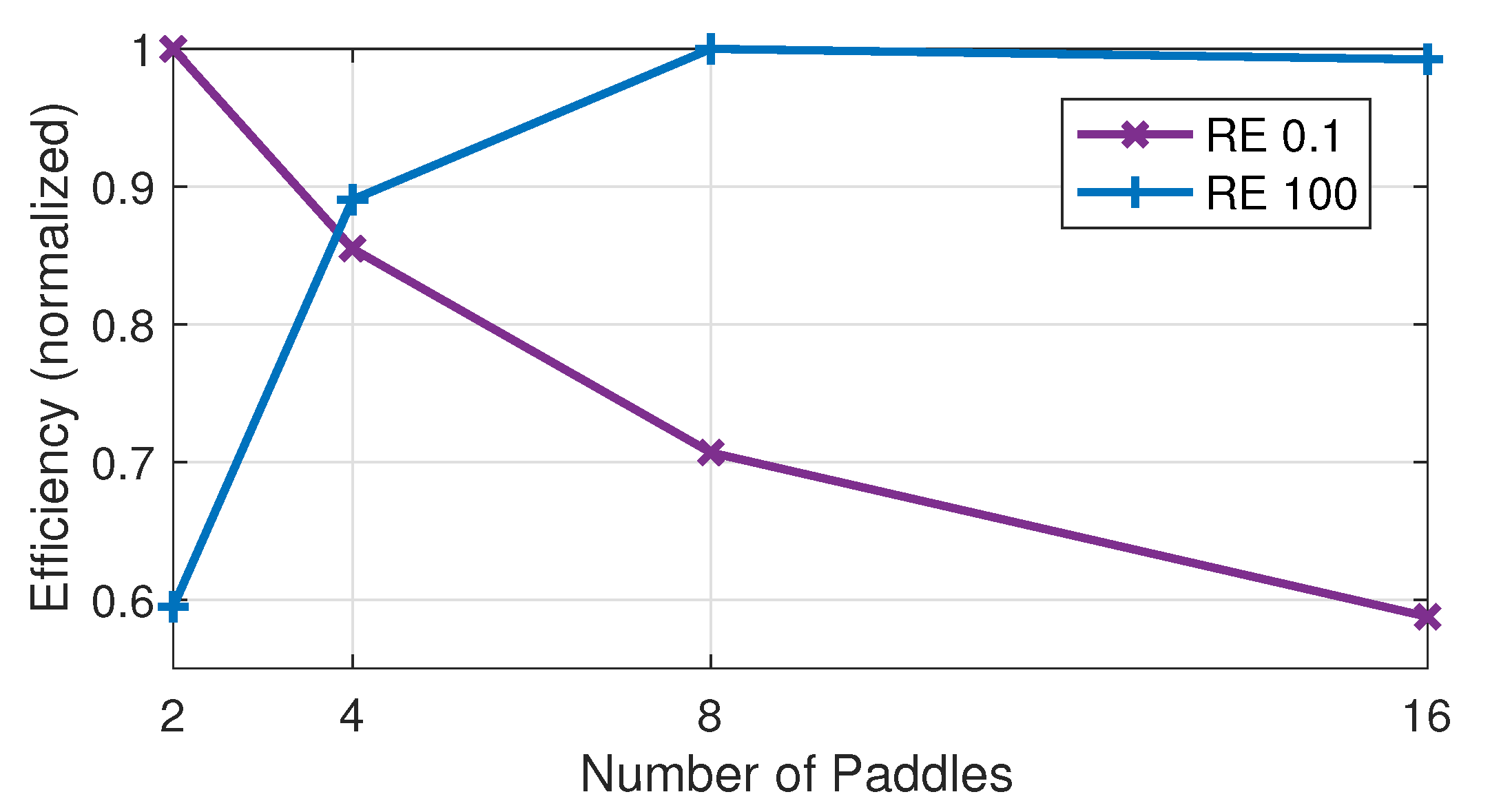
In Figure 10, paddling efficiency is plotted as a function of the number of paddles at RE 0.1 (low) and 100 (intermediate). The computations were run on a domain of length 20 to accommodate the large number of paddles. The paddles were spaced by $0.375$, they beat with a 25% phase difference, and the efficiency was computed over the 10th period. The efficiency is normalized by its maximum for each RE. At RE 0.1 the maximum efficiency occurs at two paddles, and the efficiency decreases as the number of paddles increases. In contrast, at RE 100, the minimum efficiency occurs at two paddles, and the efficiency increases as the number of paddles increases up to eight paddles at which it achieves the maximum efficiency (the efficiencies for eight and 16 paddles are nearly the same).

These results indicate small numbers of paddles are more efficient at low RE, and large numbers of paddles are more efficient at intermediate RE. Interestingly with four paddles the system paddles at 85%–90% of maximum efficiency at both low and intermediate RE. This point is notable given that many crustaceans, ranging from copepods that paddle at very low RE to krill which paddle at intermediate RE, have three to five pairs of limbs [12].

4. Discussion

Long-tailed crustaceans maintain an approximate quarter-period phase-difference between neighboring abdominal limbs independent of paddling frequency (0.1 to 10 Hz) [2]. As the swimmer moves forward, the paddling frequency itself can and do change over time, but the time-lag between the movements of neighboring limbs (ipsilaterally) must be dynamically maintained at about 25% of the paddling period to produce the limb movements necessary for coordinated locomotion [13]. How neighboring limbs or body segments maintain appropriate motor coordination for effective locomotion over a broad range of frequencies, a phenomenon known as phase constancy, has been an area of intense study in neuroscience [13,14]. Recent works [8,15,16] have revealed that the asymmetric neuronal network connectivity in the crayfish central nervous system provides a robust neural mechanism to generate and maintain this 25% phase constancy in their metachronal propulsion. Our results here show that the optimality of the approximate 25% phase-difference between neighboring paddles is robust to changes in Reynolds number, and therefore it is robust to changes in the paddling frequency and the swimmer size.

The robustness of the phase-difference across size scales is notable given that many crustaceans from small scales to large scales paddle with the same rhythm. Notable also is that the small copepods that paddle at very low Reynolds to large long-tailed crustaceans that operate at much larger Reynolds numbers generally have three to five limbs. We demonstrated that this number of limbs is near optimal in efficiency at both low and intermediate Reynolds numbers. As animals develop over the course of their lives, they function at different size scales, and hence Reynolds numbers. For example, in early stage development, Artemia (brine shrimp) larvae only have one pair of limbs, and in the later developmental stages, additional pairs of limbs appear, and the newly formed limbs beat with the existing limbs with a metachronal rhythm [6]. This increase in the number of paddles corresponds to an increase in Reynolds number from about 2 to 40 and is consistent with our numerical results that a higher number of paddles is preferred as Reynolds number increases from close to 0 to 100.

While the optimal phase-difference does not depend on Reynolds number, we found that the optimal spacing between limbs does change with Reynolds number. In particular, our results demonstrate a Reynolds number transition around 80 which is characterized by the presence of vortex shedding and vortex interaction away from the paddles. Our results are consistent with [9] who report very little vortex interaction and very little vertical flow at Reynolds number 50. As discussed in [9] the vertical flow is needed to produce lift, which is likely important for larger animals that are not neutrally buoyant.

Our results show the significance of limb spacing on paddling performance, but the values of our paddle spacing are not directly comparable to reported values of crustacean limb spacing. In crustaceans that use metachronal paddling, the ratio of the space between the base of the limbs to the length of the limbs is in the range 0.2 to 0.65 [3]. By contrast, the spacing range we explore, $w=0.2$ to $w=0.6$, relative to the paddle length ($\ell =0.15$) is in the range 1.3 to 4. In our model, tighter limb spacing would result in collisions between the paddles. We could use smaller spacing with lower amplitude strokes, but the amplitude that we use is comparable to the amplitudes reported in [3]. Crustaceans are able to paddle with this large amplitude and small limb base spacing without colliding because they bend on return stroke and their mean angles with the body are not uniform. Given the constraint of our simpler kinematics, we can only match the limb spacing or the amplitude. We chose to match the amplitude for two reasons. First, it is the amplitude of the stroke that sets the length scale of the shed vortices, and second we conjecture that the key spacing to consider is the spacing of the tips of the limbs as they paddle. In crustacean paddling, the bending of limbs and variable angles at the body greatly amplify the spacing at the tips compared to the base when compared to a model with straight limbs and fixed angles with the body. It would be interesting to revisit the question of limb spacing with kinematics more like those seen in nature.

Finally, we note that our model paddles were symmetric in their forward and backward stroke. The limb structure of long-tailed crustaceans allow its effective paddle surface area to expand during power stroke to increase propulsion and to shrink by bending at joints during return stroke to reduce drag. In this work, however, we decided not to include this additional asymmetry so that we can focus on the effects of the asymmetry in the phasic movements of limbs. There are other features of crustacean paddling not captured in our model such as difference in the mean angle of the limb or variations in the amplitude. We note that the recent results from [11] highlighted the significance the additional asymmetry in the mean angle at low Reynolds number. Using two paddles with a phase difference of $\Delta \varphi =0.25$, they observed no net motion of their robot swimmer when the mean angle of both paddles was $\overline{\alpha }=\pi /2$. However, they obtained forward locomotion when the mean angles of both paddles were titled away from the center, introducing additional asymmetry. Using our computational model with the kinematic parameters of [11] at Reynolds number 0.1, we observed a small positive flux with the mean angle for both paddles at $\overline{\alpha }=\pi /2$. We then included the extra 20 degree tilt outward on the mean angle of both paddles, and the flux increased by 250%. The details of the paddling kinzematics clearly affect the flux, and as our results on paddle spacing suggest, the optimal kinematics and arrangement likely depends on the Reynolds number. Nevertheless, we believe that our results on the presence of a Reynolds number transition and the optimum paddling rhythm may be generally applicable to more complex paddling motions.