Abstract
Various organisms such as crustaceans use their appendages for locomotion. If they are close to a confining boundary then viscous as opposed to inertial effects can play a central role in governing the dynamics. To study the minimal ingredients needed for swimming without inertia, we built an experimental system featuring a robot equipped with a pair of rigid slender arms with negligible inertia. Our results show that directing the arms to oscillate about the same time-averaged orientation produces no net displacement of the robot each cycle, regardless of any phase delay between the oscillating arms. The robot is able to swim if the arms oscillate asynchronously around distinct orientations. The measured displacement over time matches well with a mathematical model based on slender-body theory for Stokes flow. Near a confining boundary, the robot with no net displacement every cycle showed similar behavior, while the swimming robot increased in speed closer to the boundary.
1. Introduction
A diversity of organisms rely on the coordination of multiple appendages for locomotion. Examples include various crustaceans such as copepods [1], remipedes [2], krill [3,4], crabs [5], and lobsters [6,7]. There is commonly a phase delay between the oscillation of adjacent appendages, which collectively produce a rhythm referred to as a metachronal wave [8,9,10]. The metachronal wave typically travels along the body of the swimmer in the direction of locomotion [4,6,11]. The swimming performance depends on numerous factors, which include the shape, amplitude, phase, and number of oscillating appendages [4,10,12,13].
Here we consider the basic physical ingredients needed to swim with rigid appendages through a viscous fluid with small inertia. This is partly inspired by the locomotion of microscopic crustaceans operating in a physical regime of low Reynolds number. In this physical regime, locomotion requires cycles of non-reciprocal motion in order to overcome the dominant effects of viscosity [14]. A common strategy adopted by microscopic organisms is to rely on many flexible flagella and cilia beating collectively in a metachronal rhythm [15,16], though other organisms such as larval copepods have relatively stiff and smaller number of appendages. Our previous experiments showed that two rigid arms are sufficient for generating flow, provided that there is a phase difference between the oscillating arms [17]. However, the arms were fixed in place and not mobile. There is a fundamental difference between the fluid flow fields around fixed and mobile arms because the fixed arms are subjected to a net force, while the mobile arms can be force-free in the limit of negligible inertia. Flow generation does not necessarily imply locomotion. Thus, further research is needed to understand the minimal ingredients for locomotion.
Here we report a series of experiments designed to study the motion of a simple robot with a pair of rigid arms. The arms are dipped in silicone oil, while the rest of the robot is placed on a linear air track so that it is able to move freely along the horizontal track. The position of the robot was tracked over time and compared with a previously developed model based on the slender-body theory for Stokes flow [12]. Although the theory neglects the effects of inertia and confinement which are present in the experiments, the predictions match reasonably well with the experimental data. Our study offers novel insight into the significance of directing the arms to oscillate about distinct orientations for propulsion. This may have some implications for the morphology of tiny crustaceans such as larval copepods, which have three pairs of legs radiating out from their small rounded body.
2. Materials and Methods
The experimental system featured a robot equipped with a pair of rigid arms that were immersed in a tank of silicone oil as sketched in Figure 1a. The arms were each actuated by a servo motor (TowerPro SG90) and labeled as Arm 1 and Arm 2 (Figure 1b). Each arm was 3D printed with Acrylonitrile Butadiene Styrene (ABS) plastic and shaped into a rigid rod of length mm and diameter mm. The robot was designed to glide on a virtually frictionless surface of an air track system (Eisco PH0362A) such that it could translate freely along the linear track. The ridge-shaped track prevented the robot from rocking or veering off the horizontal track. The air track was fixed onto two adjustable platform stands (Wisamic 8“ × 8“ Lab Jack) to raise or lower the height of the robot as needed. The arms were dipped to a depth of mm below the surface of a large cylindrical bath of silicone oil with total depth 190 mm, diameter 300 mm, and kinematic viscosity mm2/s at room temperature.
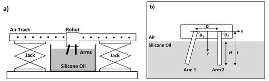
Figure 1.
(a) Sketch of the experimental setup. The air track is placed on top of two jacks. The robot glides on the air track and the arms of the robot are dipped in a tank of silicone oil. (b) The arms are of length mm and separated by a distance mm. They are dipped mm into a tank of silicone oil. The orientation angles of Arms 1 and 2, and , respectively, are controlled by servos.
The robotic arms were controlled by a microcontroller (ATmega328P) and a wireless module (XBee XB24CZ7WIT-004 and communicated using XCTU) powered by a 9 V battery. The two arms were programmed to pivot around two axes separated by a distance mm. This separation distance needed to be sufficiently large to avoid collisions and hydrodynamic interactions, which were neglected in our theoretical analysis. The horizontal directions from one pivot along and across the line to the other pivot are denoted by x and y axes, respectively. Each arm was set to oscillate periodically over time t such that the angle to the x axis changed according to
where A is the amplitude, is the angular speed, is the phase difference, and is the median angle of the ith arm. In this study we varied and in three separate cases (Table 1). In Case 1, is set to zero, meaning that the two arms move synchronously. In Cases 2 and 3, the two arms move asynchronously with a phase difference of . In Case 2, the two arms have distinct median angles, whereas in Case 3, the median angles are identical. The amplitude was fixed to and the angular frequency was fixed to rad/s, corresponding to an oscillation period of s. The Reynolds number of the fluid flow was computed to be , which is much smaller than 1. Thus the inertia of the oil is expected to play a minor role in the experiments. The inertia of the robot may have a more significant effect because a large proportion of the mobile body is not immersed in the oil. The combined mass of the mobile robot on the air track was measured to be 255 g.

Table 1.
Parameters varied in the three experimental cases: phase difference and the median orientation angles and of the two arms.
To study the effects of a nearby boundary on the dynamics of the robot, we performed the three cases with a smaller gap h between the floor and the tips of the arms (Figure 2a). This was achieved by adjusting both the height of the air track and the depth of the silicone oil in a shallower rectangular tank with dimensions of 610 mm × 457 mm × 76 mm. To introduce additional confinement effects, we inserted two transparent walls perpendicular to the floor at a distance w away from the arms, as sketched in Figure 2b.
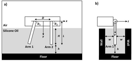
Figure 2.
(a) The arms are at a distance h away from the floor. (b) When vertical walls were introduced, they were at a distance w from the arms.
The air track was levelled carefully each time the distance h to the floor was varied. First, we ensured that the robot, with its arms powered off, remained stationary on the track with the air pump turned on. If the track were not sufficiently level, the robot would have drifted down the track due to gravity. Second, we verified that the robot, with its arms actuated in Case 1, showed the same behavior moving in one direction as in the opposite direction, resulting in no net displacement every cycle. The two jacks were adjusted as needed until we observed the expected behavior on a horizontal track. Once the air track was calibrated, each run was recorded for a minute, which corresponds to approximately 14 cycles. The position of the robot was recorded at 30 frames per second (Sony Alpha A6000 camera) and tracked using an open source tracking software (Tracker). The data were analyzed and plotted in MATLAB.
3. Results
The displacement of the robot changes with time as shown in Figure 3. In Case 1 with the arms moving synchronously, the body moves back and forth with minimal displacement at the end of each cycle. In Case 2 with the arms moving asynchronously, the body moves back and forth but drifts slowly in one direction, resulting in locomotion. In Case 3, even though the arms are moving asynchronously, the body again shows minimal displacement after each cycle. There are some variations in the net displacement every cycle, possibly caused by time-varying forces on the robot. For example, the lift force from the air track may fluctuate slightly over time because of unsteady air flow from the discrete set of holes on the air track, though the exact origin of the fluctuations is unclear. Nevertheless, the variations are small in magnitude and showed no systematic changes in displacement in Cases 1 and 3 as in Case 2. This shows that the key parameter for swimming with rigid arms is not only the phase difference but also the orientation of the arms.
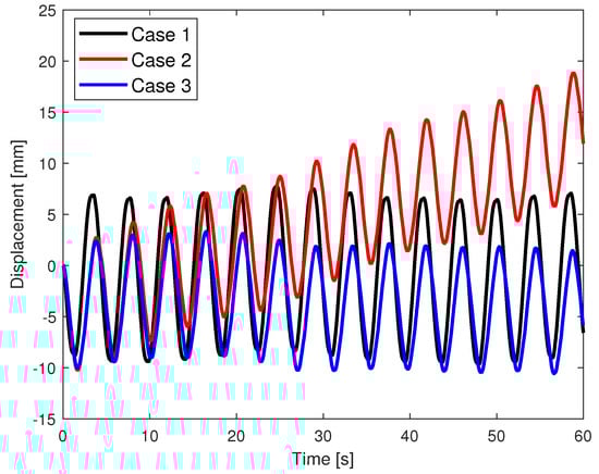
Figure 3.
The displacement of the robot when the arms move synchronously (Case 1), asynchronously with distinct median angles (Case 2), and asynchronously with same median angles (Case 3).
The orientation angles of the arms and the displacement of the robot within one cycle are shown in Figure 4. 14 cycles were averaged and the mean and standard deviation at each time step are plotted. In Case 1, when the arms reverse the direction of motion at the time points of 0.25 and 0.75 into the periodic cycle, the robot still has momentum and does not immediately reverse its motion. There is a short time lag when the robot reverses direction due to small inertial effects. As a result, the robot does not return to its original position after half the periodic cycle. Nevertheless, after a full periodic cycle, there is minimal displacement in Case 1 ( mm) and Case 3 ( mm) compared to Case 2 ( mm). The displacement curves in Cases 2 and 3 are similar at the beginning but differ toward the end of the cycle.
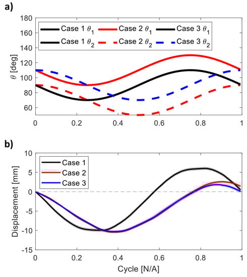
Figure 4.
(a) Orientation angles of the two arms within one cycle for the three cases. (b) The mean displacement per cycle of the robot in the three experimental cases tested. The mean is obtained by taking the average over 14 cycles and the standard deviation is shown by the shaded region.
The effect of a rigid boundary was investigated by placing the arms at a closer distance h to the floor (Figure 2a). In Case 1 with synchronous arms, the displacement of the robot over time is almost identical near the floor ( mm) and far away from the floor ( mm), as shown in Figure 5. In Case 2, interestingly, the net displacement per cycle increases from to mm as the robot is placed closer to the floor. There is no noticeable difference in the displacement of the robot in Case 3 closer to the floor.
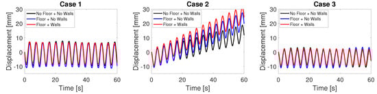
Figure 5.
Displacement of the robot in the three cases when it is far away from the floor ( mm), near the floor ( mm), and near the floor and wall ( mm and mm).
The net displacements per cycle at different distances h are shown in Figure 6. As h decreases, the net displacement per cycle remains around zero in Case 1 and Case 3. In Case 2, the net displacement per cycle increases slightly from mm at mm to mm at mm. Then it increases more significantly to mm at mm. The robot in Case 2 is able to swim at higher speed as it gets closer to the floor.
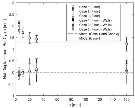
Figure 6.
The net displacement per cycle at different distances h away from the floor. Markers show the net displacements per cycle, averaged over 14 cycles. Error bars show associated standard deviations. The circle, square, and diamond markers correspond to Cases 1–3, respectively. The filled markers were obtained with the arms confined by additional walls. Dashed lines show the expected net displacements per cycles according to Equation (4).
We introduced additional confinement effects by inserting two vertical walls on both sides of the arms at a distance mm away (Figure 2b). There was no noticeable difference in the displacement of the robot in Cases 1 and 3, as shown in Figure 5 and Figure 6. In Case 2, the net displacement per cycle further increased to mm after introducing the walls in addition to the floor around the arms.
4. Discussion
In our experimental system, there is an air-oil interface above the rigid arms. But the flow field around the two arms is equivalent to that around four arms completely immersed in silicone oil, which is obtained by constructing a reflected image as sketched in Figure 7. The original set of two arms and the surrounding flow of oil can be readily reflected across the air-oil interface as long as the interface remains flat, an approximation that is expected to be valid when the flow generated by the arms is sufficiently weak. The equivalence arises because the stress-free boundary condition at the flat interface is satisfied automatically by the symmetric flow at the plane of reflective symmetry.
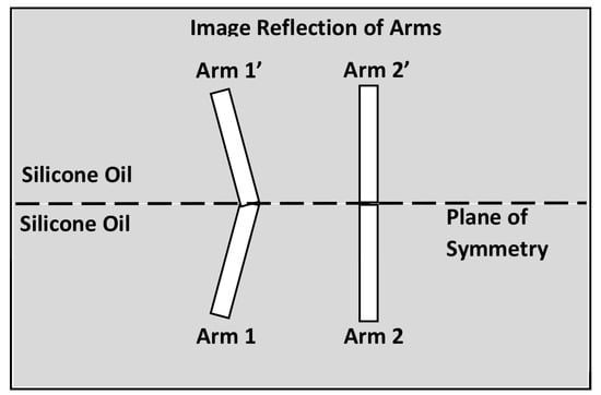
Figure 7.
An image system featuring a symmetric robot immersed completely in silicone oil. This system is obtained by reflecting the region below the air-oil interface.
We analyze and interpret our experimental results using a mathematical model of a swimmer having rigid slender legs [12]. The model neglects inertia and confinement effects. For a body of negligible size equipped with two pairs of arms, the model predicts that the velocity of the body at any instant is given by
in units of arm length L per period T. Equation (3) is integrated numerically to obtain the displacement over time. The predicted displacement in the model is compared with the experimental data in Figure 8. Overall, there is very good agreement between the predicted and measured data when the robot is far away from the floor and walls.
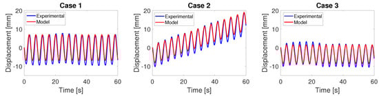
Figure 8.
The theoretically predicted displacement of the robot compared with the experimentally measured data, obtained with the robot far away from the floor and walls.
The model also predicts that, if the orientation angles of the arms oscillate with a small amplitude A in radians, the expected displacement every cycle is given by [12]
The expected displacement is proportional to the square of the amplitude A and to . Changing the sign of the phase difference changes the sign of , meaning that the swimming direction depends on the metachronal wave of the oscillating arms. Interestingly, the swimming direction depends also on the two median angles and . Figure 9 shows the expected displacement every cycle as a function of the two median angles, with the phase difference fixed at and the amplitude set at . If the arms have the same median angle, , then we expect no displacement every cycle, which is consistent with our observations. If the arms oscillate asynchronously around two distinct orientations, then the body is expected to swim in general. The swimming direction reverses if the two median angles are switched. The displacement is maximized when the two median angles are and radians, where is about 41.5 degrees, obtained from setting the derivative of Equation (4) to zero.
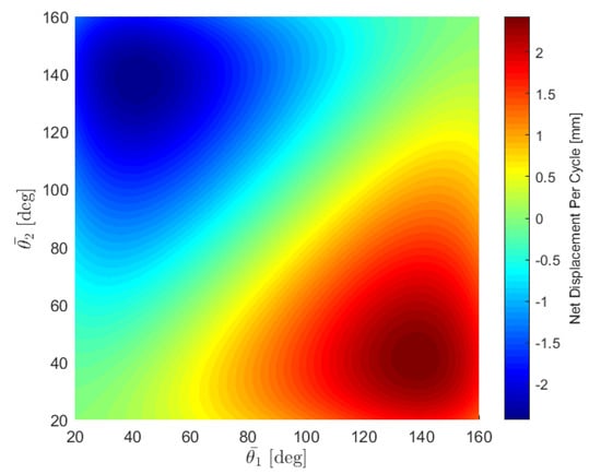
Figure 9.
Net displacement per cycle as a function of the median angles with a constant phase difference of /2 and amplitude of 20.
The predicted net displacement per cycle matches very well when the arms are far away from the floor ( mm) but begins to deviate only in Case 2 as the arms get closer to the floor shown in Figure 6. Interestingly, the swimming speed increases as the robot arms are confined further by the floor and the walls. Similar results have been previously reported with different type of swimmers in confinement [7,18,19,20,21,22,23,24,25]. For instance, a microswimmer modeled as an infinite waving sheet is able to swim faster near parallel walls with an increase in the rate of working by the sheet [18]. The effect of boundaries in our experiments could be partly explained by adopting the method of images in theory, a technique for imposing the no-slip condition on the boundary by introducing a suitable combination of Stokeslets across the boundary. To a first approximation, the flow around a single robot at a distance h to a boundary is equivalent to that around a pair of robots, one corresponding to a mirror image of the other, swimming in tandem with a separation distance . A pair of robots having the swimming gait (as in Case 2) could reinforce each other’s flow and thereby increase the swimming speed as h decreases. While this would provide some insight into the boundary effects, further research is needed to fully explain the physical boundary effects. In the future the model could be extended to account for the finite dimensions of the arms and the presence of confining boundaries by using regularized Stokeslets and the method of images [26].
Our experimental system offers exciting opportunities to explore additional effects in the future. For example, the Reynolds number could be increased by adjusting the angular speed of the arms to generate inertial jets of relevance to larger crustaceans crawling along a boundary [7]. However, the results must be interpreted carefully if the air-oil interface deforms substantially. The interface must remain nearly undisturbed in order to have the immediate correspondence to a fully immersed body. Another example is to replace the rigid arms with a body equipped with flexible arms. Instead of prescribing their orientations over time, the oscillatory driving forces on them could be prescribed to better model a swimming organism. Finally, the fluid flow generated around mobile arms could be investigated. We suspect that non-swimming robots may still hover and generate intriguing flow patterns around them.
Author Contributions
Conceptualization, R.H. and D.T.; Data curation, R.H.; Formal analysis, R.H. and D.T.; Funding acquisition, D.T. All authors have read and agreed to the published version of the manuscript.
Funding
This research was funded by the National Science Foundation, grant number CBET-1603929.
Conflicts of Interest
The authors declare no conflict of interest.
References
- Lenz, P.H.; Takagi, D.; Hartline, D.K. Choreographed swimming of copepod nauplii. J. R. Soc. Interface 2015, 12, 20150776. [Google Scholar] [CrossRef]
- Kohlhage, K.; Yager, J. An analysis of swimming in remipede crustaceans. Phil. Trans. R. Soc. 1994, 346, 213–221. [Google Scholar]
- Murphy, D.W.; Webster, D.R.; Kawaguchi, S.; King, R.; Yen, J. Metachronal swimming in Antarctic krill: Gait kinematics and system design. Mar. Biol. 2011, 158, 2541–2554. [Google Scholar] [CrossRef]
- Zhang, C.; Guy, R.D.; Mulloney, B.; Zhang, Q.; Lewis, T.J. Neural mechanism of optimal limb coordination in crustacean swimming. Proc. Natl. Acad. Sci. USA 2014, 111, 13840. [Google Scholar] [CrossRef] [PubMed]
- Plotnick, R.E. Lift based mechanisms for swimming in eurypterids and portunid crabs. Trans. R. Soc. Edinb 1985, 76, 325–337. [Google Scholar] [CrossRef]
- Davis, W.J. Quantitative analysis of swimmeret beating in the lobster. J. Exp. Biol. 1967, 48, 643–662. [Google Scholar]
- Lim, J.L.; DeMont, M.E. Kinematics, hydrodynamics and force production of pleopods suggest jet-assisted walking in the American lobster (Homarus americanus). J. Exp. Biol. 2009, 212, 2731–2745. [Google Scholar] [CrossRef]
- Knight-Jones, E.W. Relations between metachronism and the direction of ciliary beat in Metazoa. Q. J. Microsc. Sci. 1954, 95, 503–521. [Google Scholar]
- Morgan, E. The swimming of Nymphon gracile (Pycnogonida): The swimming gait. J. Exp. Biol. 1972, 56, 421–432. [Google Scholar]
- Alben, S.; Spears, K.; Garth, S.; Murphy, D.; Yen, J. Coordination of multiple appendages in drag-based swimming. J. R. Soc. Interface 2010, 7, 1545–1557. [Google Scholar] [CrossRef]
- Alexander, D.E. Kinematics of swimming in two species of Idotea (Isopoda: Valvifera). J. Exp. Biol. 1988, 138, 37–49. [Google Scholar]
- Takagi, D. Swimming with stiff legs at low Reynolds number. Phys. Rev. E 2015, 92, 023020. [Google Scholar] [CrossRef] [PubMed]
- Ford, M.P.; Lai, H.K.; Samaee, M.; Santhanakrishnan, A. Hydrodynamics of metachronal paddling: Effects of varying Reynolds number and phase lag. R. Soc. Open Sci. 2019, 6, 191387. [Google Scholar] [CrossRef] [PubMed]
- Purcell, E.M. Life at low Reynolds number. Am. J. Phys. 1977, 45, 3. [Google Scholar] [CrossRef]
- Lighthill, J. Flagellar hydrodynamics. SIAM Rev. 1976, 18, 161–230. [Google Scholar] [CrossRef]
- Brumley, D.R.; Polin, M.; Pedley, T.J.; Goldstein, R.E. Metachronal waves in the flagellar beating of Volvox and their hydrodynamic origin. J. R. Soc. Interface 2015, 12, 20141358. [Google Scholar] [CrossRef]
- Hayashi, R.; Takagi, D. Asynchronous oscillations of rigid rods drive viscous fluid to swirl. Phys. Rev. Fluids 2017, 2, 124101. [Google Scholar] [CrossRef]
- Katz, D.F. On the propulsion of micro-organisms near solid boundaries. J. Fluid Mech. 1974, 64, 33–49. [Google Scholar] [CrossRef]
- Felderhof, B.U. Swimming and peristaltic pumping between two plane parallel walls. J. Phys. Condens. Matter 2009, 21, 204106. [Google Scholar] [CrossRef]
- Felderhof, B.U. Swimming at low Reynolds number of a cylindrical body in a circular tube. Phys. Fluids 2010, 22, 113604. [Google Scholar] [CrossRef]
- Liu, B.; Breuer, K.S.; Powers, T.R. Propulsion by a helical flagellum in a capillary tube. Phys. Fluids 2014, 26, 011701. [Google Scholar] [CrossRef]
- Shum, H.; Gaffney, E.A. Hydrodynamic analysis of flagellated bacteria swimming in corners of rectangular channels. Phys. Rev. E 2015, 92, 063016. [Google Scholar] [CrossRef] [PubMed]
- Wu, H.; Thiebaud, M.; Hu, W.F.; Farutin, A.; Rafai, S.; Lai, M.C.; Peyla, P.; Misbah, C. Amoeboid motion in confined geometry. Phys. Rev. E 2015, 92, 050701. [Google Scholar] [CrossRef] [PubMed]
- Liu, C.; Zhou, C.; Wang, W.; Zhang, H.P. Bimetallic Microswimmers Speed Up in Confining Channels. Phys. Rev. Lett. 2016, 117, 198001. [Google Scholar] [CrossRef] [PubMed]
- Demir, E.; Yesilyurt, S. Low Reynolds number swimming of helical structures in circular channels. J. Fluids Struct. 2017, 74, 234–246. [Google Scholar] [CrossRef]
- Ainley, J.; Durkin, S.; Embid, R.; Boindala, P.; Cortez, R. The method of images for regularized Stokeslets. J. Comp. Phys. 2008, 227, 4600–4616. [Google Scholar] [CrossRef]


© 2020 by the authors. Licensee MDPI, Basel, Switzerland. This article is an open access article distributed under the terms and conditions of the Creative Commons Attribution (CC BY) license (http://creativecommons.org/licenses/by/4.0/).