Article

Energy Transport by Kelvin-Helmholtz Instability at the Magnetopause

by
Francesco Palermo
Max-Planck-Institut für Plasmaphysik, Boltzmannstr. 2, 85748 Garching bei Munchen, Germany
Fluids 2019, 4(4), 189; https://doi.org/10.3390/fluids4040189
Submission received: 1 September 2019 / Revised: 14 October 2019 / Accepted: 18 October 2019 / Published: 1 November 2019
(This article belongs to the Special Issue Modelling of Plasma Flow)

Abstract

:
By means of the formation of vortices in the nonlinear phase, the Kelvin Helmholtz instability is able to redistribute the flux of energy of the solar wind that flows parallel to the magnetopause. The energy transport associated with the Kelvin Helmholtz instability contributes significantly to the magnetosphere and magnetosheath dynamics, in particular at the flanks of the magnetopause where the presence of a magnetic field perpendicular to the velocity flow does not inhibit the instability development. By means of a 2D two-fluid simulation code, the behavior of the Kelvin Helmholtz instability is investigated in the presence of typical conditions observed at the magnetopause. In particular, the energy penetration in the magnetosphere is studied as a function of an important parameter such as the solar wind velocity. The influence of the density jump at the magnetopause is also discussed.

1. Introduction

The environment around the Earth magnetopause represents an important natural laboratory for plasma physics, where multifaceted phenomena occur and interact in a not fully understood manner. The magnetopause is the interface between the static plasma of the magnetosphere and the shocked solar wind that flows in the magnetosheath. This transition region moves in and out in response to solar wind variations. In fact, the magnetopause motion is principally driven by pressure fluctuations and the magnetic field orientation of the solar wind. When the interplanetary magnetic field lines related to the solar wind are antiparallel to that of the terrestrial field, reconnection phenomena act at the subsolar point with an injection of energy and mass from the solar wind to the magnetosphere. During this phase a strong motion of the magnetopause is observed [1,2,3]. When the interplanetary magnetic field is northward, the reconnection mechanism is quenched, but a large activity in the plasma dynamics is observed in particular at the flank of the magnetopause. The magnetopause waves can be excited by the Kelvin Helmholtz (KH) instability due to the velocity shear layer generated between the solar wind and the magnetosphere. In fact, the KH instability may occur when there are two regions with a relative motion across a transition layer. For its characteristics, this instability is ubiquitous in nature and it is involved in a large variety of problems in several fields of the physics. This instability is commonly observed in the Earth’s clouds, ocean surfaces, atmospheres of Jupiter and Saturn but also in the solar corona [4] and so on. Recently, it has been demonstrated that the KH instability can play an important role also in the zonal flow dynamics of the tokamak devices [5,6,7]. Generally, this instability is presented as a mechanism of saturation able to dissipate the energy related to the velocity shear layer. Theory and gyrokinetic simulations showed that KH instability can act, not only as a mechanism of saturation for the velocity shear, but also as a mechanism of generation of convective structures such as the zonal flow [6,8]. An important aspect is that the KH instability can be inhibited by a magnetic field aligned with the velocity flow. Thus, in the space-plasma context, the most favorable conditions for the development of the KH instability are at the flanks of the magnetopause, where the magnetic field of the solar wind and geomagnetic field lines are almost perpendicular to the plane of inhomogeneous velocity flow. In the past decades, considerable attention has been given to the KH instability at the magnetosphere boundary for its role in the energy transport in the magnetosphere. The transport effects associated with the KH instability can, in principle, contribute significantly to this energy flux.
The energy transfer process between the solar wind and the magnetosphere represents one of the fundamental problems in the magnetospheric physics and for this reason, the KH instability at the magnetopause conditions has been extensively studied. Concerning this problem, one of the first models [9] suggested a viscous interaction along the flank of the magnetopause by which the solar wind energy can enter by a diffusive process the magnetosphere. With this consideration, the problem was shifted to determine the nature of this viscous interaction and its contribution to the magnetosphere convection in order to better understand the solar wind magnetosphere interaction. Successively a complementary energy transfer mechanism from the solar wind to the magnetosphere has been conjectured by Lemaire in Ref. [10] via surface distortion of the magnetopause, but without transport of mass. It is important to note that the ion-ion viscosity by Coulomb collisions is extremely negligible in this context to justify the necessary viscous tangential stress. Consequently, the viscosity in the magnetopause layer must be due essentially to some anomalous plasma process. Therefore, the different mechanisms able to generate anomalous viscosity process have been examinated.
Thus, several works [11,12,13] have shown that KH instability in its nonlinear phase is able to generate an anomalous viscosity along the flanks of the magnetopause through which the solar wind energy and momentum can enter by diffusive process in the magnetosphere and validating in this way the viscosity model [9]. Evidence of KH instability at low latitude magnetopause flanks has been reported in different papers [14,15]. KH vortices signatures are identified by analyzing data of Geotail spacecraft with northwards interplanetary magnetic field [16]. The development of KH instability at the flanks of the magnetopause has been evidenced with a comparison between THEMIS data and nonlinear simulations [17,18]. Kelvin Helmholtz vortices have also been observed on both of the Earth’s magnetotail regions [15]. Numerical works on 2D magnetohydrodynamics (MHD) simulations [16] have shown that during the development of nonlinear phase the KH instability can twist up the magnetic field lines, leading to magnetic reconnection inside the vortices. In this way, the KH instability facilities not only the magnetospheric entry of energy and momentum on the equatorial flanks of the magnetopause but also the entry of mass.
Moreover, it has been shown that the secondary reconnection instability is able to disrupt the vortex structure, so as to change the large scale evolution significantly [16].
Another important secondary vortex mechanism that can strongly influence the magnetic reconnection inside the vortex is the Rayleigh Taylor (RT) instability [19,20]. This instability is driven by the alternating density layers constituted by solar and magnetosphere plasma respectively that roll-up in the KH vortex arms in which the centrifugal acceleration acts as an “efficient gravity”. 3D Hall-MHD simulations showed that KH instability is able to spontaneously generate magnetic reconnection at mid-latitude changing the global topology of the magnetic field [18]. Further studies on the development of KH instability in 3D geometry performed with Hall-MHD models have been recently performed [21,22,23]. In particular, it has been evidenced the presence of regions where trapped particles gain energy before escaping [24]. All these elements contribute to characterize the properties through which the energy can enter in the magnetosphere via the primary KH instability. An important parameter that strongly influences the KH vortex dynamics is the amplitude of the shear velocity. It has been demonstrated that in compressible conditions, for homogeneous case, the velocity jump must be less that twice the fast magnetosonic velocity for the existence of an unstable KH regime [11,25]. However, additional unstable modes can exist over this velocity jump radiating energy from the shear layer [26,27]. In the magnetopause the shocked solar wind regains a fraction of its initial speed as it flows past the magnetosphere [28] and, at the same time, the plasma temperature decreases more and more [29]. In particular, near the magnetopause flanks, the magnetosheath plasma is increasingly accelerated as the distance from the Earth increases. Moreover, the tension related to the magnetic field lines can further accelerate the plasma in the magnetosheath allowing it to reach velocities larger than that of the solar wind in space [30].
Therefore, the range of velocity in the magnetosheath is extremely large and the amplitude of velocity shear layer can significantly influence the transport properties of the low latitude of the magnetopause. In Ref. [31], with an ideal MHD model, the authors estimate the energy transport and suggest that plane waves generated by the KH instability can transport energy away from the velocity shear layer.
However, the problem of energy transfer is further complicated by the eventual presence of shocks. In fact, at high velocities, the vortex acts as an obstacle and possibly leads to the formation of shocks structures. These structures extend far from the transition region and have been studied in several numerical works in the purely hydrodynamic limit [32], in the ideal MHD limit [33,34,35] or with more complex two-fluid models [36,37]. Furthermore, during the shock formation, strong rarefaction, and compressional effects occur in the central transition region thus modifying the non-linear processes (pairing, secondary instabilities) observed in the slow magnetosonic Mach number regime [38].
Thus, the problem of energy transfer between solar wind and magnetosphere required new careful and devoted studies. A realistic evaluation of the transport rate and non-ideal MHD effects are important in order to understand more deeply the transfer process of energy, and possibly mass from solar wind into the magnetosphere.
In this paper the geometry discussed in Ref. [36] is adopted. Starting from fixed profiles of several quantities, the amplitude of the shear velocity is varied, in order to study the transition from the low magnetosonic Mach number to super magnetosonic regimes with typical Mach numbers of order one or larger. Within this representation, the energy flux connected with the development of the KH instability is estimated at several velocity values of the shear flow. The influence of density jump between magnetosphere and magnetosheath is also discussed.
Thus, after to have presented in Section 2 the numerical model used in this work, the obtained results are discussed in Section 3. Finally, the conclusions of the work are presented in Section 4.

2. Numerical Method

In this study, an ion-electron two-fluid plasma description is adopted in order to model the system. The considered equations are written in dimensionless form and all quantities are normalized by means of characteristic values. In particular for the system the following normalization are considered: the inverse of the ion gyrofrequency for the time, the ion inertial scale length d i = c / ω p i . In d i expression, ω i is the ion plasma frequency and c is the speed of light. The velocities are normalized with the Alfvén velocity c A . In the rest of the paper, the subscript i , e indicates the ion and the electron species respectively. Thus, the equations in dimensionless conservative form are as follows:
n t + · ( n U ) = 0
( n U ) t + · n ( u i u i + d e 2 u e u e ) + P I ¯ ¯ BB = 0 ,
where U = u i + d e 2 u e is the fluid velocity, P = P i + P e the pressure and n = n i n e the density (quasi-neutrality is assumed).
In this investigation an adiabatic closure is adopted, in order to well describe the formation of shocks.
( n S e , i ) t + · ( n S e , i u e , i ) = 0 ,
where S e , i = P e , i n γ and where a polytropic index γ = 5 / 3 is assumed. The dimensionless sound velocity is defined as c s = ( γ P / n ) 1 / 2 . The electric field is calculated by means of the generalized Ohm’s law [39] that includes electron inertia effects:
( 1 d e 2 2 ) E = u e × B 1 n P e + d e 2 u i × B + 1 n · [ n ( u i u i u e u e ) ] .
Electron and ion velocities are calculated by combining the fluid velocity U and the current J = n ( u i u e ) = × B in which the displacement current is neglected. Finally, the magnetic field is calculated by solving the Faraday equation
B / t = × E
For this study, a 2D L x × L y spatial domain with 3D fields is taken. Periodic boundary conditions are imposed along the y direction corresponding to the solar wind direction and open transparent boundary conditions are adopted along the inhomogeneous x direction. In the central region of the box, where the KH instability develops, the system spontaneously can generate smaller scales with phenomena regulated by a two-fluid dynamics. However, far from the center towards the boundaries, it is expected that the plasma dynamics remains of the MHD type. For this reason the transparent conditions are obtained by using an ideal MHD set of hyperbolic equations, for which it is possible to define projected characteristics along the x direction [40]. In this way any MHD waves that can be produced in the central region (where the dynamics develops) are free to leave the domain without influence the system. Moreover, there are no MHD waves entering in the domain from the lateral boundaries along the full duration of simulations. Numerical stability is achieved by means of filters, a spectral filter along the periodic y-direction and a sixth-order spectral-like filtering scheme along the inhomogeneous x-direction [41]. This filtering lets the code be dissipative only at a spatial scale smaller than the d e scale. In this way, by considering zero resistivity and zero viscosity in the model, the KH vortices present an essentially inviscid evolution at large scale, and eventually magnetic reconnection at small scale. It is important to note that finite electron inertia effects included in the two fluids model provide an efficient mechanism by means of the magnetic reconnection that can act in collisionless plasma. When particular phenomena involve scales of length d e , the electrons decouple their motion (such as the ions at the scale d i ) from that one of the magnetic field. At this scale the magnetic reconnection can act inducing a change of the global magnetic field topology.

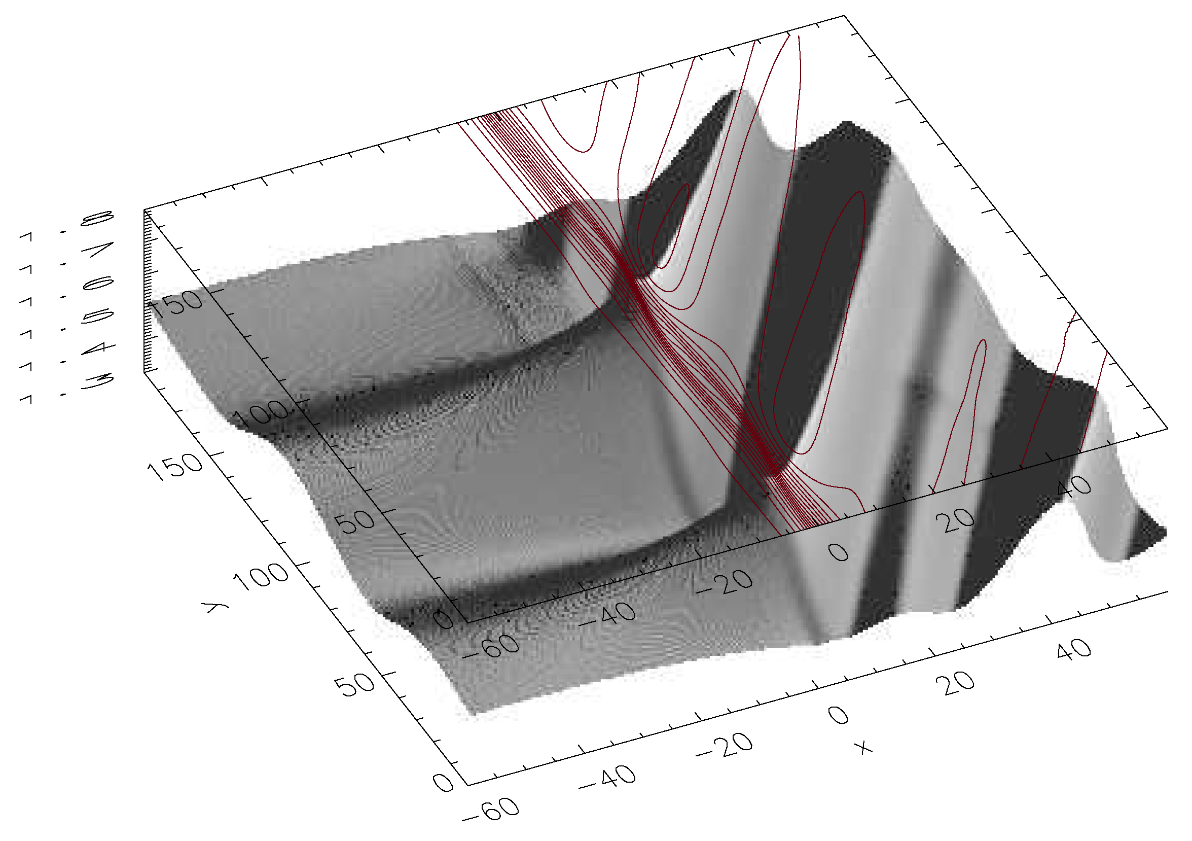
3. Simulation Results

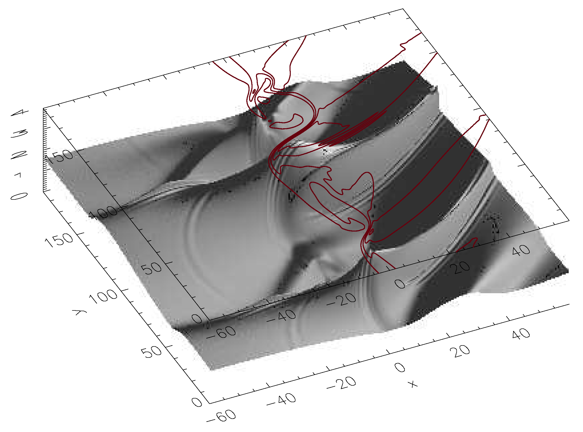
3.1. Plasma Configuration

Here, the results of two fluid simulations are presented on the KH instability that develops at the magnetopause conditions. In particular, the influence of the velocity shear is considered on the global energy transfer process in the magnetosphere. According to the satellite observations, the plasma density increases from the magnetosphere to the magnetosheath while the temperature decreases in the same direction. In the ( x , y ) box, the initial equilibrium state is based on hyperbolic tangent functions along x with the transition layer centered in L x / 2 corresponding to x = 0 . In the left side (L-side) of the box x < 0 , the magnetosphere region is reproduced and in the right side (R-side) of the box x > 0 , the magnetosheath region is represented. The initial state of the simulation uses a Galilei transformation for the velocity, such that the simulation frame moves at half the velocity of the magnetosheath plasma. The following initial background velocity in the ± y direction is assumed:
V e q = V 0 2 tanh ( x / L e q ) y ^ ,
where L e q is the thickness of the velocity shear layer. For semplicity, all the following quantities vary on the same scale length L e q .
The initial density jump is considered:
n ( x ) = n 0 Δ n 2 ( 1 tanh ( x / L e q )
and the following temperature profiles are taken:
T e , i ( x ) = T 0 ; e , i + Δ T e , i 2 ( 1 tanh ( x / L e q )
where Δ n , Δ T e and Δ T i are density, electron and ion temperature jump between the magnetosheath and magnetosphere plasma, T 0 , e + T 0 , i = 1 , n 0 = 1 . All quantities are normalized using the characteristic values at the magnetosheath side (the outermost region). Note that the plasma density increases from the magnetosphere to the magnetosheath, while the temperature decreases according to satellite observations.
The magnetic field B 0 ( x ) is chosen such that the sum of the thermal pressure and the magnetic pressure is initially uniform in the x direction:
P ( x ) + B 0 ( x ) 2 2 = c o n s t a n t
In agreement with the low latitude magnetosphere–magnetosheath conditions during northwards magnetic field configurations, a magnetic field almost perpendicular to the x y plane is considered with the components B y ( x ) = B 0 ( x ) sin θ and B z ( x ) = B 0 ( x ) cos θ . The numerical box sizes are L x = 120 and L y = 60 π and a grid mesh d x d y 0.1 in units of the ion inertial length. The numerical box is large enough compared to the typical size of the vortex structures expected after the development of the Kelvin Helmholtz instability in the central region of the box. The mass ratio is fixed to m i / m e = 64 . Finally, the following other quantities are chosen: Δ n = 0.9 , Δ T i = 2.4 , Δ T e = 0.4 , T 0 , i = 0.6 , T 0 , e = 0.4 and L e q = 3 corresponding to a transition layer larger than the ion inertial length.

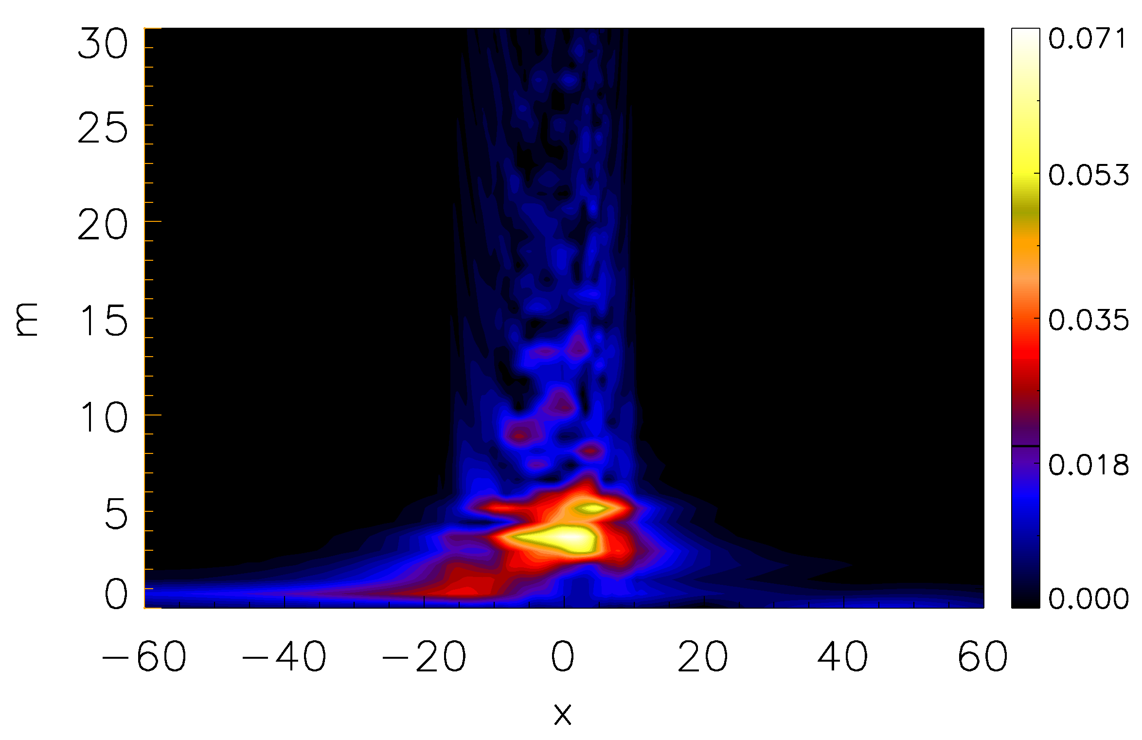
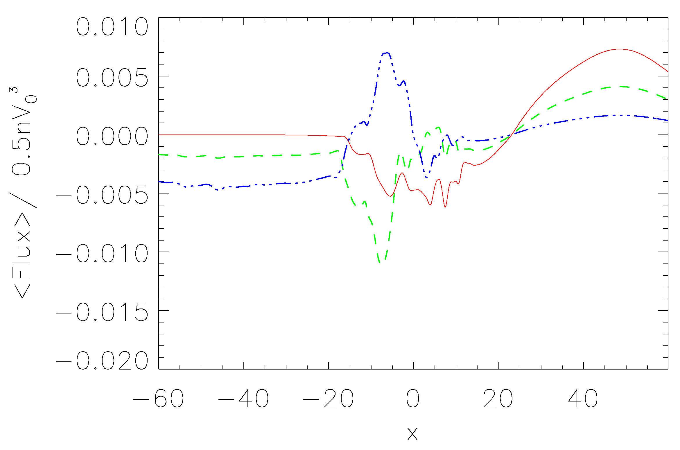
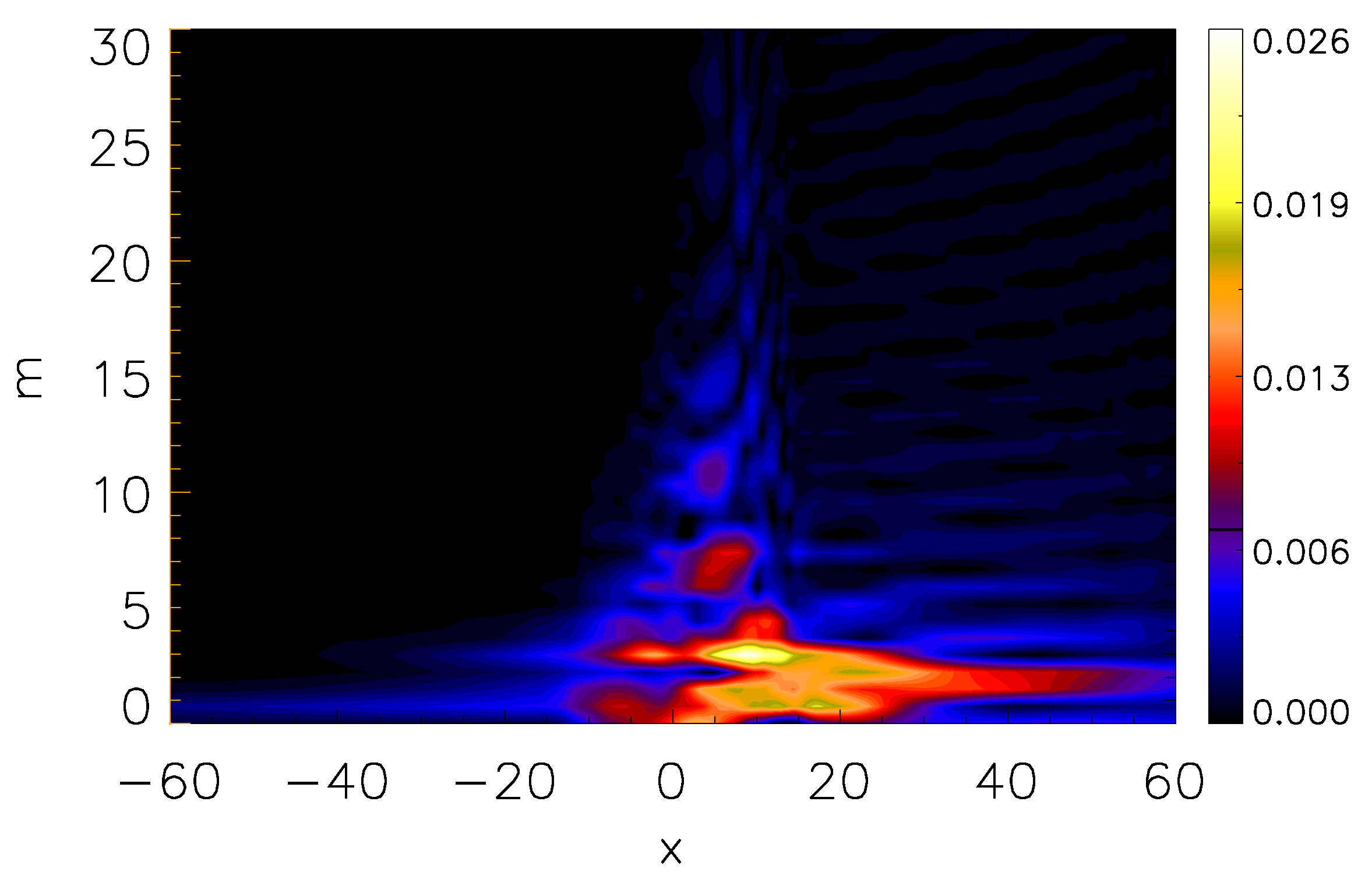
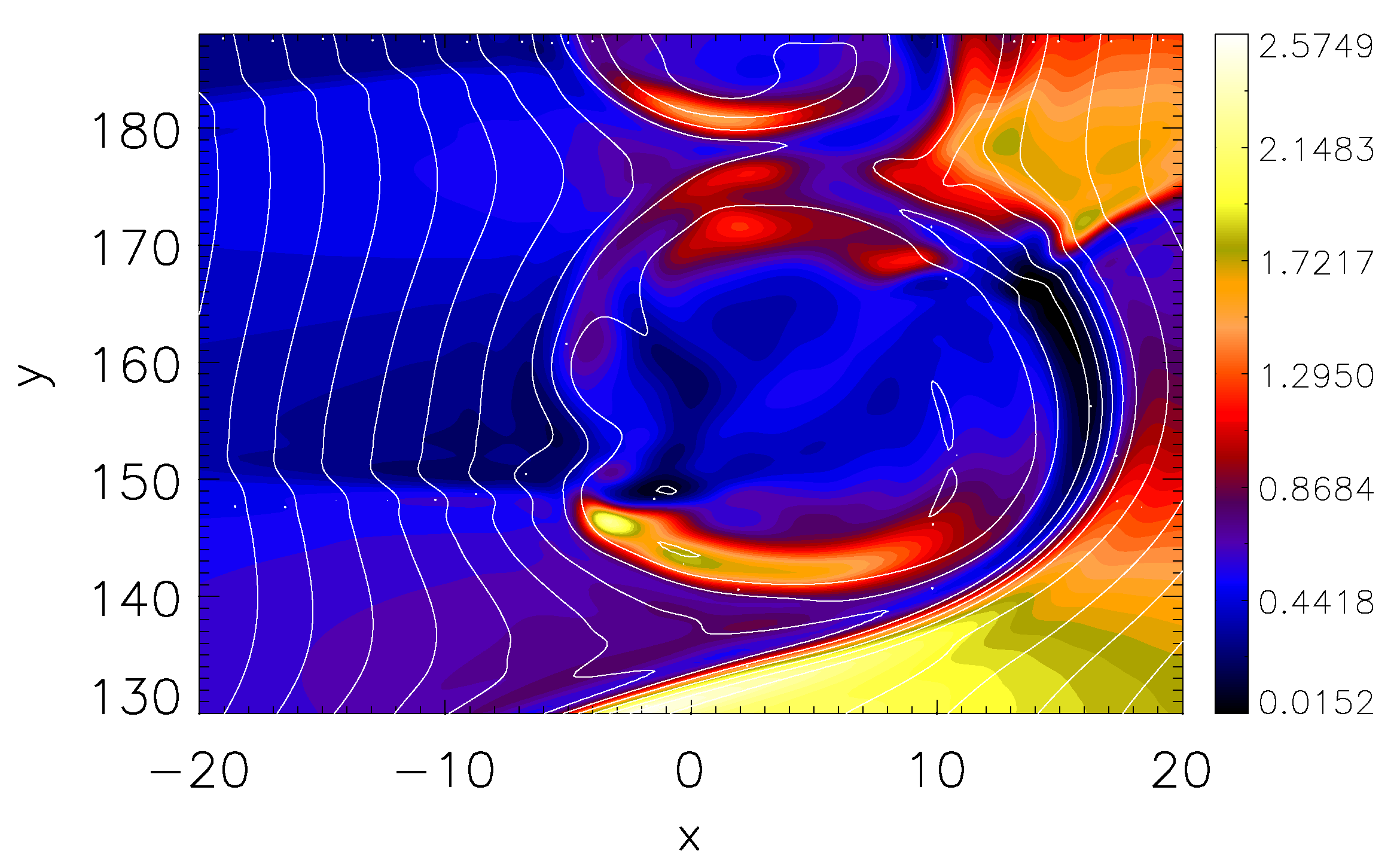
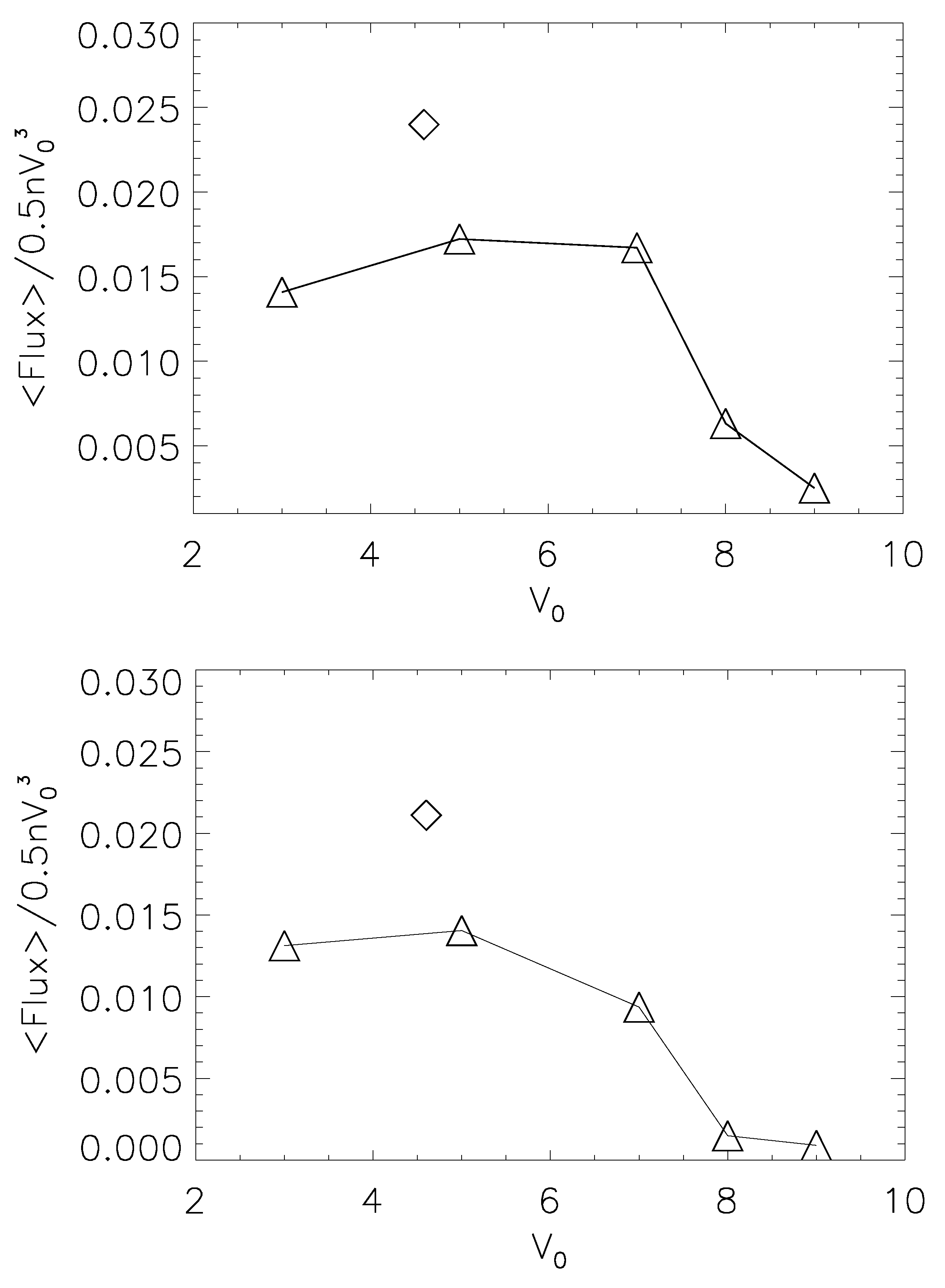
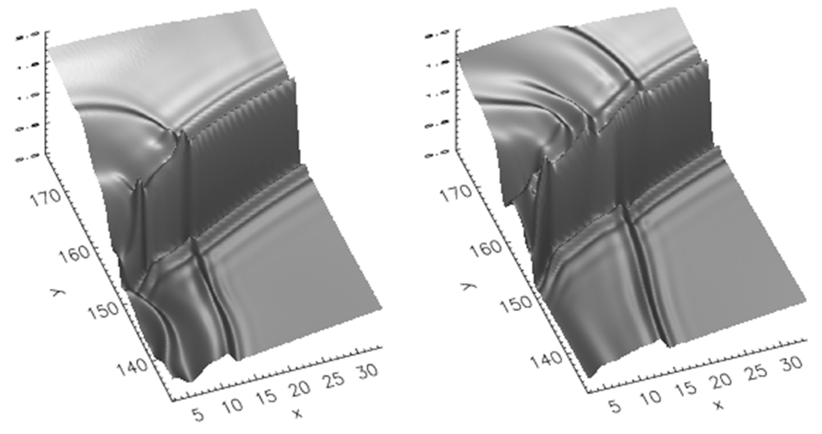
3.2. Energy Flux by Kelvin Helmholtz (KH) Instability

By means of the formation of vortices, the KH instability is able to redistribute the flux of energy characterizing the initial state of a system. In this way, the flux of energy initially parallel to the velocity shear layer is partially injected perpendicularly to the flow direction. The efficiency of this mechanism involves a huge amount of processes such as energy cascade dissipation on small scales, emission of wave perturbations and so on. For these reasons the estimation of energy transport via KH instability into magnetosphere is a very complex problem that need to be clarified and quantified. In order to investigate this problem, the following energy conservation expression can be written:
t E = · F E = 1 2 n V · V + P γ 1 + B 2 2 ,
where E is the energy density and where F = F k + F L + F B is the total energy flux density comprising the kinetic, the internal and the magnetic energy flux density term respectively. It is important to observe that the energy flux is frame-dependent. Due to the importance of the energy flux in the magnetosphere, hereafter a magnetospheric inertial frame is taken into account by means of a Galilean transformation from the original frame of the simulation box to the new frame. Thus, the dimensionless form of the three terms of the energy flux density F can be written in the magnetospheric inertial frames:
F k = 1 2 n ( V · V ) V
F L = γ γ 1 P V
F B = B 2 V ( B · V ) B ,
where V = U + V 0 / 2 y ^ and U are the velocity fields at a generic time t in the magnetosphere and in the simulation frame respectively. The average F of the energy flux density is obtained by integrating the flux along the y direction and by normalizing at the initial energy flux density 1 / 2 n V 0 3 of the magnetosheath:
F ( x , t ) = 2 n V 0 3 L y 0 L y F ( x , y , t ) d y .
Although, the energy flux density is referred to the magnetosphere frame, several characteristics of the transfer of energy depend on the relative motion between vortices and flow. Consequently, in addition to the definition of the solar wind fast magnetosonic Mach number in the Earth rest frame
M f s w = V s w / c f ; c f = ( c s 2 + c A 2 ) 1 / 2 ,
the vortex Mach number is defined as:
M f , L / R v o r t = U L / R / c f , L / R .
In Equation (14) the quantities c s , c A are the sound and Alfvén velocity, c f is the fast magnetosonic velocity calculated at the magnetosheath boundary, V s w = V 0 is the total velocity jump. In Equation (15) U represents the relative velocity of the vortex with respect to the flow in R / L -side and c f is also calculated in the respective regions. The results obtained by varying the velocity flow intensity in the range 3 < V 0 < 9 are presented. The case in which the solar wind flows with a velocity V 0 = 3 is first considered. For this case, in the linear phase a competition along the y-direction between the mode m = 5 and the mode m = 4 generates five non-uniform vortices in nonlinear phase. This is clearly evidenced in Figure 1 that shows the amplitude of the total pressure P T = P + B 2 / 2 (gray color) in the ( x , y ) -plane and overplotted the density isocontours (red color lines) at t = 146 when the saturation phase is reached.
The P T quantity is particularly useful because allows to highlight the presence of magnetohydrodynamic waves that propagate in ( x , y ) -plane. In fact, Figure 1 shows the presence of waves propagating from the shear layer where the vortex are generated. The waves move with a velocity c f that is the velocity of the fast magnetosonic waves. In the R-side the velocity of the waves is c f , R = 1.6 , while in the L-side this velocity is c f , L = 5.4 . These waves are compressional waves with a signature particularly evident on the pressure perturbation because they move perpendicularly to the magnetic field. In particular, they can move in all directions. To this purpose, each vortex and the space between them can be considered as a source of waves that propagate spherically, generating a Huygens wave front envelop that becomes more and more parallel to the y direction. This is particularly evident in the magnetosphere side. In order to better investigate the energy flux, Figure 2 shows the spectrum along the y direction for each point of the x axis. It is important to observe that the flux of energy represents the advection transport of quadratic terms. In a typical treatment of turbulence, the interpretation of this quantity in terms of energy transfer between modes is extremely complicated for the statistical character of the incoherent dynamics with a very short time memory. Fortunately, the KH instability appears as a phenomenon in which the interaction between modes has typically a coherent character with long term memory of initial conditions. In this way, it is possible to deduce several properties that appear in nonlinear phase as a normal consequence of the linear dynamics. The energy flux is concentrated in the middle of the box and on the modes m = 4 , 5 that correspond to the number of vortices generated in the box. Far from the shear layer region, lower modes are excited in particular in the magnetosphere side also as a consequence of the wave front that becomes more and more parallel to the y direction. Around x = 0 several random modes are excited at higher m due to the chaotic magnetosphere and magnetosheath plasma mixing that can be generated inside the vortices and that leads to small scale dynamics as a consequence of the development of secondary instabilities.
This chaotic behavior inside the vortex is reflected also in Figure 3 in which we plotted the x-component of the three terms F k , F L , F B of the energy flux density. In fact, inside the vortex a rapid change is observed on the intensity of the energy flux density terms that assume a negative/positive value in the L / R -side away from the center of the box. For this case the velocity of vortex is V v o r t = 0.8 (see Ref. [6]) with respect to the box frame and consequently the regime is submagnetosonics with M f , L / R v o r t < 1 in both L- and R- sides.
By increasing the velocity of the solar wind to V 0 = 5 , the effects of compressibility increase and the vortex appears as an obstacle with respect to the plasma with the consequent shock structure formation in the magnetosheath [6]. The shocks extend far from the vortex constituting another way by which the energy of the solar wind can be injected in the perpendicular direction of the magnetopause. In order to analyze this aspect, the extreme case V 0 = 7 is considered. In this case all the vortices move in the flow direction with V v o r t 1.3 corresponding to M f , R v o r t > 1 and M f , L v o r t 1 in the magnetosheath and in the magnetosphere respectively. For the case V 0 = 7 the presence of strong shocks in the R-side is observed with the simultaneous presence of weak shocks in the L-side. This is shown in Figure 4 together with the presence of fast wave propagation by means of the amplitude of the total pressure P T in the ( x , y ) -plane (gray color). The overplotted density isocontour (red color lines) puts in evidence the formation of three vortex in nonlinear phase at t = 182 .
In Figure 5, the spectrum of the energy flux density along the x direction shows that the principal modes involved in the transport of energy are the modes m = 3 , 4 that as before correspond to the number of generated vortices.
Moreover, the signature of the shocks is clearly shown in the magnetosheath where strong shocks are generated. In the shear layer, first and second harmonics of the principal mode are excited, while for x > 0 more and more higher mode are developed. As in the previous case, in Figure 6 the x-component of the three terms of the energy flux density in the saturation phase are shown. The presence of strong shocks in the solar wind allows to the flux to be extended away from the shear layer in the magnetosheath region. Instead, the flux injected in the magnetosphere is concentrated inside the vortices with a regular shape without chaotic variation. This is in agreement with the homogeneous conditions observed inside the vortices at high velocity.
To this purpose, Figure 7 shows a zoom of a vortex of Figure 4 with uniform density. The vortex is well defined from the reconnected magnetic field lines in the ( x , y ) -plane and it represents an evidence of a useful way by which a lot of mass of the solar wind can enter in the magnetosphere in the presence of a KH instability at supermagnetosonic conditions.
Increasing the velocity in the magnetosheath the limit M f , L / R v o r t = 1 is exceeded in both sides of the box and the KH instability is strongly reduced. The case V 0 = 8 shows a reduced formation of vortex structures that appears very narrow in the x direction and extended in the flow direction. In spite of this behavior, in Figure 8 for the case V 0 = 9 at t = 255 the presence of waves that propagate away from the shear layer is clearly visible. As for the case V 0 = 7 , the energy flux density (not shown) in the magnetosphere is concentrated in the middle of the box, while in the magnetosheath the intensity of the flux is low, but extends away from the shear layer.
In order to have a complete picture of the energy transfer in the magnetosphere and in the magnetosheath, in Figure 9 the maximum absolute value m a x ( | F x | ) of the flux of energy density injected in both L- and R-sides is plotted normalized to the quantity 0.5 n V 0 3 . The relative energy flux density can be considered approximately constant in the range 3 < V 0 < 7 with a value around 1.5 % of the y-kinetic energy flux density of the magnetosheath. However, a more careful analysis shows that starting from a submagnetosonic flow with respect to both of the regions of the magnetopause ( V 0 = 3 ) , by increasing the V 0 velocity the energy flux slowly increases also when the flow becomes supermagnetosonic in the magnetosheath and submagnetsosonic in the magnetosphere ( V 0 = 5 ) . When the shear flow velocity ( V 0 = 7 ) begins to be supermagnetosonic in both of the sides of the magnetopause with M f , L v o r t 1 and M R v o r t > 1 , the quantity m a x ( | F x | ) decreases. Afterwards, for a large value of the solar wind velocity V 0 > 7 , with the equilibrium conditions considered in this paper, when the flow exceeds the limit M f , L / R v o r t = 1 in both of the sides of the box, the nature of the KH unstable modes changes and the energy flow drop down.
Moreover, in Figure 9 it is also plotted the total energy flux density for a case with V 0 = 4.6 in which different equilibrium conditions with a density jump Δ n = 0.7 have been considered (see rhombus point in the figure). Moreover Δ T i = 0.6 and Δ T e = 0.4 are chosen in Equation (7). For this case, the energy flux density increases with respect to the equivalent case V 0 = 4.6 with Δ n = 0.9 . In fact, the relative flux of energy density is m a x ( | F x | ) 2.5 % . In order to understand the role played by the density in the energy flux it is important to observe that by decreasing the density jump the conditions of symmetry between the magnetosphere and the magnetosheath increase. For this case a Mach number M f , R v o r t 1 is obtained in both of the sides of the box. Thus, the formation of the shocks is even favorite in the magnetosphere and at the same time also the pairing of the vortices. The Figure 10 shows the pairing of two vortices at t = 360 for the case V 0 = 4.6 with Δ n = 0.7 , and in correspondence of the vortices the presence of shocks that extend away from the shear layer in both of the sides. Moreover, the inner of the vortices is very chaotic because of the development of secondary instabilities. These latter are evidenced by means of the generation of magnetic island due to magnetic reconnection process with several peaks in the energy flux. Due to the pairing process, part of the mass of the vortices pass through the shocks destabilizing in a first time the shocks and generating a large amount of magnetosonic perturbations. All these effects contribute in this way to increase the flux of energy density when the density jump decreases. Moreover, it is interesting to observe that because the upstream and downstream physical conditions of the shocks are very different, the energy wave emission generated from the plasma perturbations moves with different velocity in the two regions of the shocks. This is emphasized in Figure 11 that shows the generation of a perturbation at the edge of the vortices that becomes a wave-train in downstream shock region and becomes a shock in upstream region propagating along the x direction. These waves can perturb the shocks parallel to the x axis and can be at the origin of new instabilities in the magnetosphere and in the magnetosheath. A detailed study about the density jump effects will be discussed in a devoted paper.

4. Conclusions

The KH instability is a fundamental mechanism for the magnetosphere/solar wind plasma interaction at the magnetopause, responsible for a lot of phenomena, such as energy and plasma transport in the magnetosphere. This instability, via the generation of rolled up vortices, is able to change and redistribute the initial energy flux of the solar wind that flows parallel to the magnetopause. In this way, the injection of energy into the magnetosphere becomes possible. In this paper by means of a two-fluid plasma description that includes electron inertia effects, the KH evolution and the energy flux in the magnetosphere in realistic conditions have been investigated. With this model, by maintaining a fluid framework, the evolution of the KH instability has been studied including eventually collisionless reconnection process in the dynamics. In particular, starting from a fixed equilibrium configuration adopted in Ref. [36], an evaluation of the energy flux density has been done as a function of the shear flow velocity parameter. Increasing the velocity V 0 , the max value of the energy flux density increases in submagnetosonic regimes. This trend continues also when supermagnetosonic regime is reached in the magnetosheath region, but decreases when the supermagnetosonic regime is approached in both sides of the magnetopause, dropping down for higher velocities. In the submagnetosonic regime, the generation of fast waves from the KH vortex has been clearly shown. The vortices during their formation and by their rotation emit concentric waves that at large distance from the shear layer become a flat wave front. In supermagnetosonic regime the presence of shocks extends the energy flux emission far from the shear layer. Moreover, the vortices appear very homogeneous in their characteristics and this aspects is reflected also in the signature of the energy flux in the magnetosphere. Several aspects about the flux of energy as a function of the density jump have also been discussed. It has been emphasized that by decreasing the density jump and by maintaining fixed the shear velocity, the energy flux density increases due to different primary processes such as the vortex pairing in the presence of shock structures and due to the development of secondary instabilities that develop as a consequence. A detailed study about the density jump effects will be discussed in a future paper.

Funding

This research received no external funding.

Acknowledgments

Interesting and useful discussions with Omar Maj are kindly acknowledged.

Conflicts of Interest

The author declares no conflict of interest.

References

  1. Song, P.; Elphic, R.C.; Russell, C.T. ISEE 1 & 2 observations of the oscillating magnetopause. Geophys. Res. Lett. 1988, 15, 744–747. [Google Scholar]
  2. Yagodkina, O.I.; Vorobjev, V.G. Daytime high latitude pulsations associated with solar wind dynamic pressure impulses and flux transfer events. J. Geophys. Res. 1997, 102, 57–67. [Google Scholar] [CrossRef]
  3. Lee, S.H.; Zhang, H.; Zong, Q.G.; Wang, Y.; Otto, A.; Réme, H.; Glassmeier, K.H. Asymmetric ionospheric outflow observed at the dayside magnetopause. J. Geophys. Res. Space Phys. 2015, 120, 3564–3573. [Google Scholar] [CrossRef] [Green Version]
  4. Ofman, L.; Thompson, B.J. Observation of Kelvin Helmholtz instability in the solar corona. Astrophys. J. Lett. 2011, 734, L11. [Google Scholar] [CrossRef]
  5. Rogers, B.N.; Dorland, W.; Kotschenreuther, M. Generation and Stability of Zonal Flows in Ion-Temperature- Gradient Mode Turbulence. Phys. Rev. Lett. 2000, 85, 5336. [Google Scholar] [CrossRef] [PubMed]
  6. Palermo, F.; Garbet, X.; Ghizzo, A.; Cartier-Michaud, T.; Ghendrih, P.; Grandgirard, V.; Sarazin, Y. Shear flow instabilities induced by trapped ion modes in collisionless temperature gradient turbulence. Phys. Plasmas 2015, 22, 042304. [Google Scholar] [CrossRef]
  7. Ghizzo, A.; Palermo, F. Shear-flow trapped-ion-mode interaction revisited. I. Influence of low-frequency zonal flow on ion-temperature-gradient driven turbulence. Phys. Plasmas 2015, 22, 082303. [Google Scholar] [CrossRef] [Green Version]
  8. Palermo, F.; Garbet, X.; Ghizzo, A. Bicoherence analysis of streamer dynamics induced by trapped ion modes. Europ. Phys. J. D 2015, 69, 8. [Google Scholar] [CrossRef]
  9. Axford, W.I.; Hincs, C.O. A unifying theory of high-latitude. Geophysical phenomena and geomagnetic storms. Can. J. Phys. 1961, 39, 1433–1464. [Google Scholar] [CrossRef]
  10. Lemaire, J.; Roth, M. Penetration of the solar wind plasma elements into the magnetosphere. J. Atmos. Terr. Phys. 1978, 40, 331–335. [Google Scholar] [CrossRef]
  11. Miura, A.; Pritchett, P. Nonlocal stability analysis of the MHD Kelvin-Helmholtz instability in a compressible plasma. J. Geophys. Res. 1982, 87, 7431–7444. [Google Scholar] [CrossRef]
  12. Miura, A. Anomalous transport by magnetohydrodynamic Kelvin-Helmholtz instabilities in the solar wind-magnetosphere interaction. J. Geophys. Res. 1984, 89, 801–848. [Google Scholar] [CrossRef]
  13. Miura, A. Simulation of Kelvin-Helmholtz Instability at the Magnetospheric Boundary. J. Geophys. Res. 1987, 97, 3195–3206. [Google Scholar] [CrossRef]
  14. Hasegawa, H.; Fujimoto, M.; Phan, T.D.; Réme, H.; Balogh, A.; Dunlop, M.W.; Hashimoto, C.; TanDokoro, R. Transport of solar wind into Earth’s magnetosphere through rolled-up Kelvin-Helmholtz vortices. Nature 2004, 430, 755. [Google Scholar] [CrossRef]
  15. Nishino, M.N.; Hasegawa, H.; Fujimoto, M.; Saito, Y.; Mukai, T.; Dandouras, I.; Reme, H.; Retino, A.; Nakamura, R.; Lucek, E.; et al. A case study of Kelvin–Helmholtz vortices on both flanks of the Earth’s magnetotail. Planet. Space Sci. 2011, 59, 502–509. [Google Scholar] [CrossRef]
  16. Otto, A.; Fairfield, D.H. Kelvin-Helmholtz instability at the magnetotail boundary: MHD simulation and comparison with Geotail observations. J. Geophys. Res. 2000, 105, 21175–21190. [Google Scholar] [CrossRef]
  17. Palermo, F.; Califano, F.; Pegoraro, F.; Le Contel, O. Possible magnetospheric Kelvin-Helmholtz vortex signatures near the post-noon magnetopause. Mem. Soc. Astron. Ital. Suppl. 2010, 14, 189. [Google Scholar]
  18. Faganello, M.; Califano, F.; Pegoraro, F.; Retino, A. Kelvin-Helmholtz vortices and doublemid-latitude reconnection at the Earth’smagnetopause: Comparison between observations and simulations. Eur. Phys. J. 2014, 107, 19001. [Google Scholar]
  19. Matsumoto, Y.; Hoshino, M. Onset of turbulence induced by a Kelvin-Helmholtz vortex. Geophys. Res. Lett. 2004, 31, L02807. [Google Scholar] [CrossRef]
  20. Faganello, M.; Califano, F.; Pegoraro, F. Competing mechanisms of plasma transport in inhomogeneous configurations with velocity shear: The solar-wind interaction with Earth’s magnetosphere. Phys. Rev. Lett. 2008, 100, 015001. [Google Scholar] [CrossRef]
  21. Fadanelli, S.; Faganello, M.; Califano, F.; Cerri, S.S.; Pegoraro, F.; Lavraud, B. North-South Asymmetric Kelvin-Helmholtz Instability and Induced Reconnection at the Earth’s Magnetospheric Flanks. J. Geophys. Res. 2018, 123, 9340–9356. [Google Scholar] [CrossRef]
  22. Leroy, M.H.J.; Keppens, R. On the influence of environmental parameters on mixing and reconnection caused by the Kelvin-Helmholtz instability at the magnetopause. Phys. Plasmas 2017, 24, 012906. [Google Scholar] [CrossRef]
  23. Ma, X.; Delamere, P.; Antonius Otto, A.; Burkholder, B. Plasma Transport Driven by the Three-Dimensional Kelvin-Helmholtz Instability. J. Geophys. Res. 2017, 122, 10382–10395. [Google Scholar] [CrossRef]
  24. Leroy, M.H.J.; Ripperda, B.; Keppens, R. Particle Orbits at the Magnetopause: Kelvin-Helmholtz Induced Trapping. J. Geophys. Res. 2019, 124, 6715–6729. [Google Scholar] [CrossRef]
  25. Blumen, W. Shear layer instability of an inviscid compressible fluid. J. Fluid Mech. 1970, 40, 769–781. [Google Scholar] [CrossRef]
  26. Drazin, P.G.; Reid, W.H. Hydrodynamic Stability; Cambridge University Press: Cambridge, UK, 1977. [Google Scholar]
  27. Pu, Z.Y.; Kivelson, M.G. Kelvin-Helmholtz Instability at the Magnetopause’ Energy Flux Into the Magnetosphere. J. Geoph. Res. 1983, 88, 853–861. [Google Scholar] [CrossRef]
  28. Fairfield, D.H.; Otto, A.; Mukai, T.; Kokubun, S.; Lepping, R.P.; Steinberg, J.T.; Lazarus, A.J.; Yamamoto, T. Geotail observations of the Kelvin-Helmholtz instability at the equatorial magnetotail boundary for parallel northward fields. J. Geophys. Res. 2000, 105, 21159–21173. [Google Scholar] [CrossRef]
  29. Spreiter, J.R.; Summers, A.L.; Alksne, A.Y. Hydromagnetic flow around the magnetosphere. Planet. Space Sci. 1966, 14, 223–253. [Google Scholar] [CrossRef] [Green Version]
  30. Chen, S.H.; Kivelson, M.G.; Gosling, J.T.; Walker, R.J.; Lazarus, A.J. Anomalous aspects of magnetosheath flow and of the shape and oscillations of the magnetopause during an interval of strongly northward interplanetary magnetic field. J. Geophys. Res. 1993, 98, 5727–5742. [Google Scholar] [CrossRef] [Green Version]
  31. Lai, S.H.; Lyu, L.H. A simulation and theoretical study of energy transport in the event of MHD Kelvin-Helmholtz instability. J. Geophys. Res. 2010, 115, A10215. [Google Scholar] [CrossRef]
  32. Kobayashi, Y.; Kato, M.; Nakamura, K.T.A.; Nakamura, T.K.M.; Fujimoto, M. The structure of Kelvin-Helmholtz vortices with super-sonic flow. Adv. Space Res. 2008, 41, 1325–1330. [Google Scholar] [CrossRef]
  33. Miura, A. Kelvin-Helmholtz instability for supersonic shear flow at the magnetospheric boundary. Geophys. Res. Lett. 1990, 17, 749–752. [Google Scholar] [CrossRef]
  34. Miura, A. Kelvin-Helmholtz instability at the magnetospheric boundary: Dependence on the magnetosheath sonic Mach number. J. Geophys. Res. 1992, 97, 10655–10675. [Google Scholar] [CrossRef]
  35. Miura, A. Nonlinear evolution of the magnetohydrodynamic Kelvin-Helmholtz instability. Phys. Rev. Lett. 1982, 49, 779. [Google Scholar] [CrossRef]
  36. Palermo, F.; Faganello, M.; Califano, F.; Pegoraro, F.; le Contel, O. Compressible Kelvin-Helmholtz instability in supermagnetosonic regimes. J. Geoph. Res. 2011, 116, A04223. [Google Scholar] [CrossRef]
  37. Palermo, F.; Faganello, M.; Califano, F.; Pegoraro, F.; Le Contel, O. The Role of the magnetosonic mach number on the evolution of Kelvin Helmholtz vortices. Europ. Conf. Lab. Astroph. 2012, 58, 91–94. [Google Scholar] [CrossRef]
  38. Palermo, F.; Faganello, M.; Califano, F.; Pegoraro, F.; Le Contel, O. Kelvin-Helmholtz vortices and secondary instabilities in super-magnetosonic regimes. Ann. Geophys. 2011, 29, 1169–1178. [Google Scholar] [CrossRef] [Green Version]
  39. Valentini, F.; Trávníček, P.; Califano, F.; Hellinger, P.; Mangeney, A. A hybrid-Vlasov model based on the current advance method for the simulation of collisionless magnetized plasma. J. Comp. Phys. 2007, 225, 753–770. [Google Scholar] [CrossRef]
  40. Faganello, M.; Califano, F.; Pegoraro, F. Being on time in magnetic reconnection. New J. Phys. 2009, 11, 063008. [Google Scholar] [CrossRef]
  41. Lele, S.K. Compact finite difference schemes with spectral-like resolution. J. Comput. Phys. 1992, 103, 16–42. [Google Scholar] [CrossRef]
Figure 1. Total pressure P T (gray color) in the ( x , y ) -plane with overplotted density isocontour lines (red color) at t = 146 for the case V 0 = 3 . The density isocontour evidences the shape of the vortices in the middle of the box and the pressure perturbations put in evidence the emission of fast waves from the shear layer.
Fluids 04 00189 g001
Figure 2. Spectrum of the energy flux density F x along the y direction for each x point in the ( x , k y ) plane at t = 146 for the case V 0 = 3 .
Fluids 04 00189 g002
Figure 3. The x-component of energy flux density averaged along the y coordinate for the three quantities F k (red line), F L (green line) and F B (blue line) at t = 146 for the case V 0 = 3 .
Fluids 04 00189 g003
Figure 4. Total pressure P T (gray color) in the ( x , y ) -plane with overplotted density isocontour lines (red color) at t = 182 for the case V 0 = 7 . The density isocontour evidences the shape of the vortices in the middle of the box and the pressure perturbations put in evidence the emission of fast waves from the shear layer and the shock structures that extend in both sides of the box.
Fluids 04 00189 g004
Figure 5. Spectrum of the energy flux density F x along the y direction for each x point in the ( x , k y ) plane at t = 182 for the case V 0 = 7 .
Fluids 04 00189 g005
Figure 6. The x-component of the energy flux density averaged along the y coordinate for the three quantities F k (red line), F L (green line) and F B (blue line) at t = 182 for the case V 0 = 7 .
Fluids 04 00189 g006
Figure 7. Isocontour of pressure P = P e + P i with overplotted magnetic field in the ( x , y ) -plane at t = 185 for the case V 0 = 7 showing a KH vortices detached from the velocity shear layer and completely plunged in the magnetosphere.
Fluids 04 00189 g007
Figure 8. Total pressure P T (gray color) in the ( x , y ) -plane with overplotted density isocontour lines (red color) at t = 255 for the case V 0 = 9 . The density isocontour puts in evidence that not vortex structures are generated in the middle of the box, but only perturbations emphasized on the pressure quantity via the emission of fast waves from the shear layer.
Fluids 04 00189 g008
Figure 9. Maximum value m a x ( | F x | ) of the energy flux density normalized to the quantity 0.5 n V 0 3 as a function of the velocity V 0 injected along the x direction in the magnetosphere (top) and in the magnetosheath (bottom).
Fluids 04 00189 g009
Figure 10. Isocontour of pressure P = P e + P i in the ( x , y ) -plane for the case V 0 = 4.6 and Δ n = 0.7 at t = 360 s. The pairing of vortices that pass through the shocks is shown. Overplotted it is shown the magnetic field in the plane with the magnetic island originated from the reconnection process in the vortices.
Fluids 04 00189 g010
Figure 11. Pressure perturbation P T in the ( x , y ) -plane for the case V 0 = 4.6 and Δ n = 0.7 at t = 360 (left) and at t = 365 (right). Due to the different conditions upstream and downstream the shocks, the perturbations originated at the edge of vortex propagate in the x-direction with different velocities in the two regions of the shock.
Fluids 04 00189 g011

