1. Introduction
Exact solutions play a special role in hydrodynamics. At pre-computer times, exact solutions served as the main tool for obtaining information about fluid motions. Classical examples of stationary isothermal solutions are the Poiseuille flow in a pipe under applied pressure drop [
1]; the Couette flow between two surfaces, one of which is moving tangentially relative to the other [
2]; the Taylor flow confined between two rotating coaxial cylinders [
3]. Each solution above describes a steady laminar fluid flow in a space with simple geometry. Together with an evident aesthetic effect, having a closed-form solution makes one understand the problem and identify the main physical mechanisms of the fluid motion.
Convective problems formulated within the Boussinesq approximation [
4] of the Navier–Stokes equations gave their exact solutions. For example, a closed-form steady solution was obtained for a vertical fluid layer differently heated from sidewalls [
5,
6]. The paper by Gershuni [
5], as well as the subsequent paper by Batchelor [
6], have opened an era of convective flow stability theory. This was followed by a large number of papers analyzing linear and nonlinear stability of this flow [
4,
7]. This shows us one more important application of exact solutions. Linear theory of the convective stability (in case of isothermal problems, it is hydrodynamic stability) studies a range of infinitesimal perturbations of the base flow. Having a closed-form exact solution for the base flow is crucial for this analysis. With no such solution, one needs to get it numerically and the analysis of infinitesimal perturbations becomes not such a justified step before a direct numerical simulation. It is finding a new exact solution that triggered a new area of research since the existence of such a solution for fluid motion questions the stability of this motion under different values of the control parameters. An elegant example of the kind is the closed-form exact steady solution found by Birikh [
8]. It describes a laminar fluid motion in a horizontal layer with a free upper surface, where the flow is generated by a longitudinal temperature gradient. Finding the solution, on the one hand, brought a lot of publications studying the stability of the flow [
9,
10,
11,
12], to mention but a few. On the other hand, one could observe the papers considering formally a whole group of similar solutions, including some time-dependent examples [
13,
14]. The most complete, but far from exhaustive, list of exact solutions of the Navier–Stokes equations is given in [
15,
16].
There are not many exact unsteady solutions for hydromechanics equations because the procedure for obtaining a solution is much more complicated [
15,
16,
17,
18]. One of the first solutions of this type was derived in 1868 by Stokes [
19], who found the structure of the viscous fluid flow, which arises as a result of harmonic oscillations of a solid plate. In 1882, Gromeka found a closed-form solution for the non-stationary isothermal motion of viscous fluid in an infinite cylindrical tube, whose ends were affected by the applied periodically pulsating pressure drop [
20,
21].
The authors of the most recent monograph on exact solutions of the Navier–Stokes equations [
15] state that the term an
exact solution denotes a solution which has a simple explicit form, usually an expression in finite terms of elementary or other well known special functions. This is in contrast to an
approximate solution, which is taken to be a field, simple or complicated, which approximates a solution either in a numerical sense or in an asymptotic limit. The monograph [
15] gives the following classification of exact solutions to the Navier–Stokes equation based on their temporal and geometric constraints. The most general criterion determining the type of solution is its dependence on time. If the fluid motion conditions change over time, such a solution is unsteady. On the other hand, the geometry of the problem imposes its limitations on the type of solution. Two important classes of solutions are distinguished respectively for flows bounded by plain walls and cylindrical geometry [
15]. The first class includes, for example, the plane Couette–Poiseuille flow, Beltrami flows, stagnation-point flows, and channel flows. The second one includes circular and non-circular pipe flows, generalized Beltrami flows, rotating-disk flows, and some others. A more rigorous mathematical classification of exact solutions can be based on Ovsyannikov’s group analysis of differential equations [
22]. One can mention other works devoted to the general mathematical classification of a closed-form exact solution of hydrodynamics including both stationary and non-stationary cases [
23,
24,
25].
A further important development of the research on thermal convection was the paper by Baxi, Arpaci, and Vest [
26], which unfortunately was published in an inaccessible book chapter. They seem to be first to derive a closed-form unsteady solution for the thermal convection in a differently heated vertical slot subjected to the gravity modulation. Later, a similar solution was independently found by Gershuni, Keller, and Smorodin [
27] for the case of the finite-frequency vibrations applied to a non-uniformly heated fluid layer performing periodic harmonic vibrations of the low frequency along with the layer in weightlessness. Since the convective flow solution found is quite physical (in contrast to non-stationary variants of Ostroumov–Birikh’s flow [
14]), and the behavior of the convective system in microgravity conditions is a quite topical area for research recently, several works have appeared to study the stability of this flow by applying the Floquet theory [
26,
27,
28,
29,
30,
31]. It turned out that it is possible to find similar solutions for inhomogeneous media. Bratsun and Teplov [
32,
33] have shown that the solution [
26,
27] can be generalized to the case of a dusty medium (fluid with small solid particles). Since the flow is significantly non-stationary, one should take into account the effect of the non-stationary friction forces between the fluid and solid phases on the stability of the flow [
34].
In the past several decades, the interaction between reaction–diffusion phenomena and pure hydrodynamic instabilities has attracted increasing attention on the part of researchers in nonlinear science and chemical engineering [
35,
36]. The interest arises from the fact that the chemically induced changes of fluid properties such as density, viscosity, thermal conductivity, or surface tension may result in instabilities that exhibit a large variety of convective patterns. Authors are actively involved in these studies [
37,
38,
39] and this was one more motivation to write this article. While the convective destabilization of the mechanical equilibrium of the reacting fluid is well studied, the processes that take place in the reacting flow are still poorly investigated.
In this communication, we focus on several problems of thermo- and chemovibrational convection, in each of which the closed-form unsteady solutions of the convection equations will be obtained. An important difference between these solutions and those considered in the monograph [
15] is the presence of an additional field (temperature or concentration), which makes the hydrodynamic system spatially inhomogeneous in density, which means the sensitivity of this system to the external inertial action. Thus, these solutions are non-generic and cannot be considered as typical representatives of solutions to the Navier–Stokes equations. The purpose of the paper is to demonstrate the possibilities in designing various one- and two-dimensional exact solutions of the above type, which should attract the attention of researchers to these problems both from the point of view of the general analysis and formulating the issue about the stability of the obtained time-dependent flows.
2. General Formulation
The hydrodynamic system that we consider is a closed cavity filled by an incompressible fluid, which is subjected to the action of a non-stationary, but regular vibrations. It is also assumed that the non-uniform density structure of the fluid was developed as a result of some process of heat and/or mass transfer. Such a process may be excited by the external heating of the fluid from the cavity boundaries, internal heat generation in the fluid due to the chemical reaction or radiation, seepage of impurities from the outside, or some other reason. In this case, the inertial force acting on the fluid element substantially depends on the density of this element and makes the fluid move.
We start with the set of reaction–diffusion–convection equations, which consists of the continuity Equation (
1), Navier–Stokes Equation (
2) coupling to evolution Equations (
3) and (
4) for the temperature
T and the concentration
C (suppose there is only one chemical species dissolved in the fluid), respectively,
where
is the velocity, and
P is the pressure. The density
of the fluid, its kinematic viscosity
, temperature diffusivity
and heat capacity
are physical constants characterizing the fluid.
stands for the kinetic function of the reactive scheme while
Q is the enthalpy of reaction. The diffusion term in (
4) has been written in the most general form taking into account the possible effect of a concentration-dependent diffusion
of species [
37,
40].
The Boussinesq approximation implies that density differences are ignored in all terms except the body force term responsible for the buoyancy effect. We assume that density variations in (
2) consist of a fixed part and other parts that have a linear dependence on temperature and concentration
where
and
stand for the coefficients of thermal and solutal expansion, respectively. In (
5), we assume that the reagent is heavier than the solvent. Thus, both coefficients are positive.
The inertial field
has a static component, gravity
, and time-dependent part representing the vibrational force
where
and
are the amplitude and frequency of vibrations, respectively.
Laminar flow can be defined as the flow that consists of infinitesimal parallel fluid layers sliding in parallel, with no eddies, swirls or currents normal to the flow itself. In our case, the laminar flow condition is the orthogonality of the density gradient and the inertial field
which is maintained at any time.
If condition (
7) is not met, then the streamlines of the flow inevitably will cross and mix, since the translational symmetry of this problem will be broken. There are two evident cases where condition (
7) is exactly satisfied. If the flow of a fluid is one-component (say
), then the density field may depend on two spatial coordinates
In the case of a two-component laminar flow (say
), the structure of the Equation (
2) is as follows:
Below, we present examples of problems for which the Navier—Stokes equation can be represented either in the form (
8) or (
9), which implies that condition (
7) is satisfied.
3. Thermovibrational Convection in an Internally Heated Fluid Layer
In this section, we examine a combined flow of incompressible fluid in a plain layer with the thickness of and highly heat-conductive walls. Let us assume that heat sources with the generation power Q are evenly distributed throughout the layer. Two physical effects trigger the flow: a constant gravity force acting along the z-axis, and a variable inertial field applied along the same axis. The time-dependent inertial field is formed by the harmonic oscillations of the cavity with the amplitude a and frequency . If the plates limiting the layer are maintained under constant equal temperatures, then the temperature field inside the layer will be invariant with respect to reflection about the mid-plane of the layer. Let us find a closed-form unsteady solution for this problem.
A heat transfer Equation (
3) is supposed to have a term which accounts for the internal heat sources
Let us assume that
Q does not depend on the coordinates and time. Since there is no external heating of the layer that could set the characteristic scale for the temperature, we construct such a unit due to the heat generation power
. Using the half-thickness
h of the layer as length scale,
as time scale,
as velocity scale and
as pressure scale, the set of Equations (
1)–(
3), (
5) and (
6) can be written in the dimensionless form
where
is the unit vectors along the
z-axis.
Boundary conditions for the velocity and the temperature are
As a result, the dimensionless parameters appearing in (
11)–(
13)
are the Grashof number based on the capacity of the heat sources, the Prandtl number, the vibration amplitude (overload parameter) and the dimensionless frequency, respectively. The weightlessness case is singular here and requires the exclusion of the gravity vector from the dimensionless parameters.
Let us assume that the equations describing the structure of the base flow remain invariant under translation and the flow remains laminar. Then, the solution can be sought in the form
In this case, the continuity Equation (
11) is automatically satisfied. One can see that the structure of the solutions (
16) corresponds to case (
8) for the one-component velocity field, which keeps the scalar product (
7) equal to zero. By taking into account (
16), we obtain
By analyzing Equations (
17) and (
18), one can conclude that
is not explicitly time-dependent, and the problem for temperature (
18) transforms to
and can be solved separately. By solving Equation (
19) with the boundary conditions (
14), we come to the following equation of motion:
Since Equation (
20) has a range of possible solutions, one should select the ones that are comprehensible in terms of physics. This takes us to one more assumption defined as follows:
which is the mass conservation of incompressible fluid in an enclosed cavity formulated for the
component. If the laminar flow is described by a two-component velocity field, condition (
21) must be met for each component separately.
At this stage, we must make one important remark. It is necessary to clearly distinguish the situations when an oscillatory excitation comes from a force acting in the bulk of a fluid (as in this work) and when it is caused by a surface force (for example, as in the Stokes problem [
19] and related problems, in the problems with an interphase boundary that can stretch or contract [
23], and so on). The Stokes problem also known as the Stokes second problem was devoted to obtaining an exact unsteady solution for the motion of a viscous fluid generated by a harmonically oscillating body (
Figure 1a). This is widely considered the simplest unsteady problem that has an exact solution for the Navier–Stokes equations. The main feature of this problem is the local character of the source of fluid motion and the role of viscosity in this mechanism of motion. In the case of an ideal fluid, when there is no adhesion of the body to the fluid, the motion generation does not occur at all. An important result of Stokes’ work was to obtain a formula for the thickness of the boundary layer where the fluid wave has been generated. The penetration depth of this wave decreases with the frequency of the oscillation but increases with the kinematic viscosity of the fluid. It turns out that the intensity of fluid motion decreases exponentially with distance from the source of motion. Thus, the Stokes flow can be defined as local and occurs in a narrow boundary layer (
Figure 1a). The main difference between our work and the formulation of the Stokes problem is that the source of fluid motion in our case is the heterogeneity of the medium arising from the density difference. It is important that the inertial force acts immediately over the entire volume of the fluid and generates a global flow. This mechanism works even when the fluid is ideal. However, the flow in a closed cavity decays immediately if the medium density becomes uniform. Technically, the switching between these two different cases occurs due to condition (
21). If an open pipe oscillates in a fluid, then a Stokes boundary flow is generated, but there is no inertial motion (
Figure 1a). If the pipe is closed, then the internal fluid starts to oscillate with the pipe. The Stokes mechanism stops working inside the pipe, but the global mechanism of inertial flow (its structure will be discussed below) is turned on (
Figure 1b).
When looking for the solution of (
20), it is more convenient to solve it in a complex form by substituting
for
(
i is the imaginary unit). Another point is that Equation (
20) can be solved with the appropriately selected pressure field. Since a variable force field is directed along the
z-axis, this should also cause pressure oscillations in the same direction. By solving Equation (
20) with the boundary conditions (
14) and the mass conservation condition (
21), we end up with the following closed-form unsteady solution
for the
z-component of velocity, pressure, and temperature, respectively. Here,
denotes the real part and
stands for
.
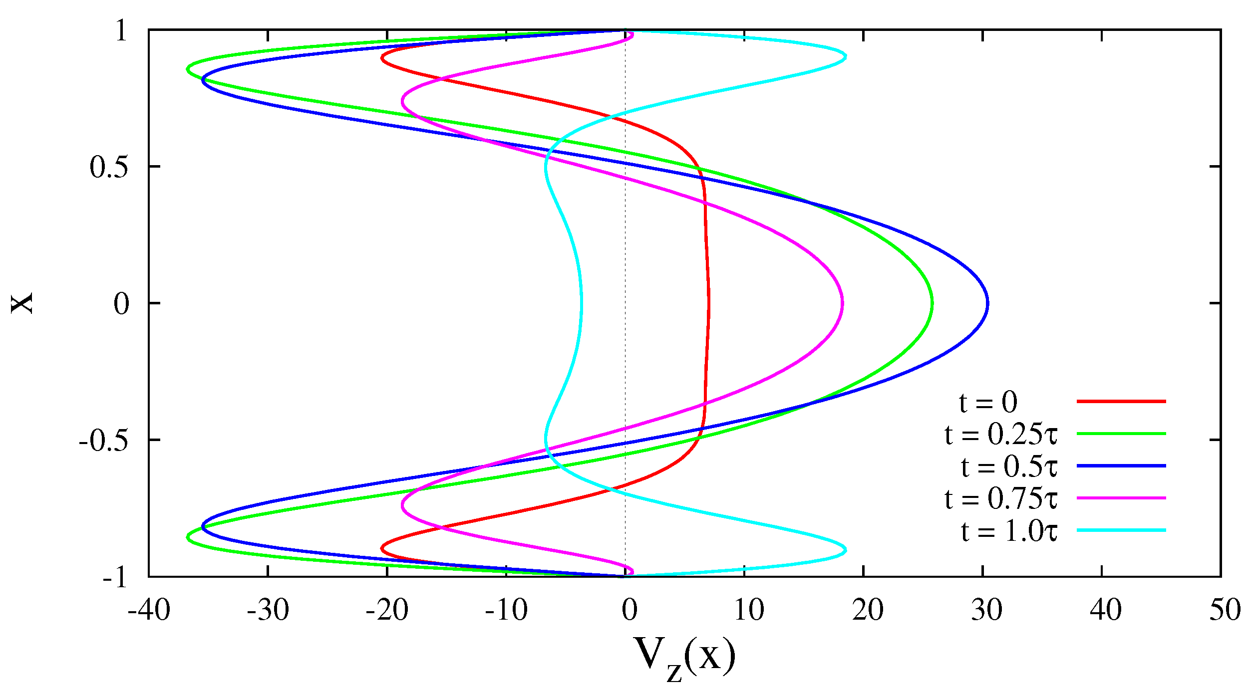
Figure 2 gives the dynamics in the velocity diagram of the base flow for the sequential times within the half-period of vibrations. The
z-component of velocity (
22) consists of two parts. The first part does not depend on time and describes the action of gravity. The second part of solution (
22) is more complicated. The main physical mechanism for fluid motion is a difference in the weights of the laminar fluid sublayers due to the internal heat generation. Heated and cold elements of the fluid have different density; therefore, they respond differently to the pulsation of the inertial field. A more agile heated laminar sublayer is the first to move, thus it pushes out the cold sublayers due to condition (
21), which results in a velocity diagram shown in
Figure 2.
4. Chemovibrational Fluid Flow in a Plain Layer
We have considered the case when the exact solutions possess particular symmetry imposed by the problem: the velocity profile is symmetric with respect to
x-axis reflection (
Figure 2). Nevertheless, if the flow remains laminar, the exact unsteady solution could also be found for the asymmetrical flow. Let us assume that the constant flux
J of a substance with concentration
C is set at the layer boundary
. The coefficient of diffusion of this species is constant and equal to
. Let us assume further that the
C is a heavier component compared to the solvent filling the layer.
The layer is subjected to the longitudinal translational vibrations, while the gravity is zero. Let us also assume that the species
C is injected into the layer, in which a first-order chemical reaction takes place
where
K is the reaction rate. Most easily, this situation can be reproduced in practice using a suitable second-order chemical reaction (for example, the chemisorption of carbon dioxide by some aqueous solution or the neutralization reaction of acid and base). One way to obtain a pseudo-first-order reaction is to use a large excess of one reactant so that, as the reaction progresses, only a small fraction of the reactant in excess is consumed, and its concentration can be considered to stay constant.
Thus, the reaction and diffusion mechanisms develop in the layer non-homogeneous stratification in density, which is why the system should be sensitive to the external inertial field. The possible effect of the heat generation within this problem will be neglected. In this case, the governing Equations (
1)–(
6) for the pure chemovibrational convection can be rewritten in the dimensionless form as
where the following units are used to adimentionalize the problem: length
h, time
, velocity
, pressure
, and concentration
.
Equations (
26)–(
28) acquire new dimensionless parameters
which are the Schmidt number, the solutal vibrational Rayleigh number, the Damkohler number, and the dimensionless vibration frequency, respectively.
The boundary conditions are defined as follows:
By analyzing the structure of Equations (
26)–(
28), we are looking for the exact solutions in the form
The equation for concentration (
28) is readily solved for the boundary conditions (
30) and (
31), and the motion equation reduces to
The partial differential Equation (
33) is solved with the properly selected pressure field. By applying the mass conservation condition (
21), we derive a closed-form unsteady solution for the asymmetric laminar flow
where we have denoted
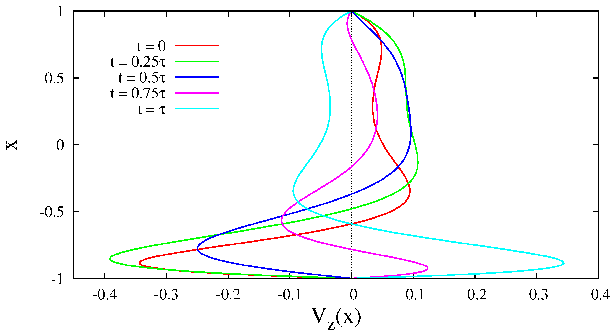
Figure 3 shows the dynamics of the base flow (
34) for several times during the half-period of vibrations
. Due to the reaction taking place, diffusion cannot level the concentration of the reactant across the layer, which creates an inhomogeneous distribution of density. It is seen from
Figure 3 that the reagent
C entering the layer at
creates a heavier (means more inert) sublayer near the wall that behaves differently under the action of an external force than a pure fluid adjacent to the boundary
. This develops the chemovibrational convection with its mechanism similar to the development of thermovibrational convection considered above. Formulas (
34)–(
37) state that a flow type significantly depends on the correlation between the typical times of reaction and diffusion determined by the Damkohler number
D. The higher the value of this parameter, the quicker the reaction is and the closer the flow runs to the wall at
. In this case, the flow increasingly becomes a boundary layer flow. With the decrease of
D, the inhomogeneity of the density is smoothed out, and the flow becomes less intense.
5. Thermovibrational Convection in an Internally Heated Cylindrical Pipe
Let us consider a more complicated example of an axisymmetric solution for the motion of a uniformly heat-generating fluid placed in an infinite cylindrical tube of circular cross-section with a radius R. This system is interesting in that it gives an example of a closed-form non-stationary spatial flow. Cylindrical geometry is often found in various applications and is popular among scholars.
Let us assume that the harmonic vibrations of the amplitude
a and frequency
are directed along the pipe, while the whole system is in a gravity-free state. We use the following units to adimensionalize the problem: length
R, time
, velocity
, temperature
and pressure
. Then, the governing Equations (
1)–(
3), (
5) and (
6) for the thermovibrational convection of fluid with the internal sources can be rewritten as follows:
where a new dimensionless parameter
is the vibrational Grashof number based on the capacity of the heat sources.
Let us assume further that non-homogeneity gradient of density and fluid velocity remain orthogonal towards each other at any moment in time satisfying condition (
7). In this case, the flow continues to be laminar, and there is only
z component of velocity which is directed along the cylinder axis. Then, the continuity Equation (
38) is again automatically satisfied. In addition, let us assume that the fluid flow is axisymmetric. By changing the coordinate system from the Cartesian to the cylindrical one, we look for the solution in the form
and obtain
The boundary conditions should be added to Equations (
43) and (
44)
In addition, one should also add the standard condition of velocity finiteness on the cylinder axis
. Temperature distribution (
42) does not depend on time; therefore, Equation (
44) can be readily solved. Inserting this solution into the motion Equation (
43), we obtain
An additional procedure to derive the solution is similar to the one described above: Equation (
46) may be written in a complex space, and all fields oscillating in time (velocity and pressure) are looked for in the form of proportional to
. Then, one can separate the variables in time and radius. Furthermore, one should meet the mass conservation condition, which in this case is
As a result, the closed-form exact solution for the unsteady fluid flow in a round tube is as follows:
where
and
stand for the Bessel functions of the first kind.
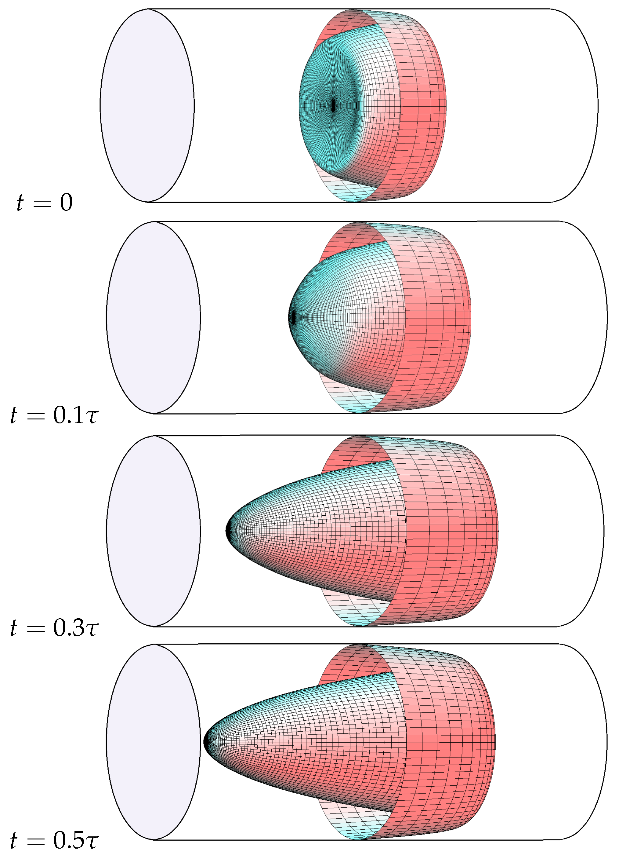
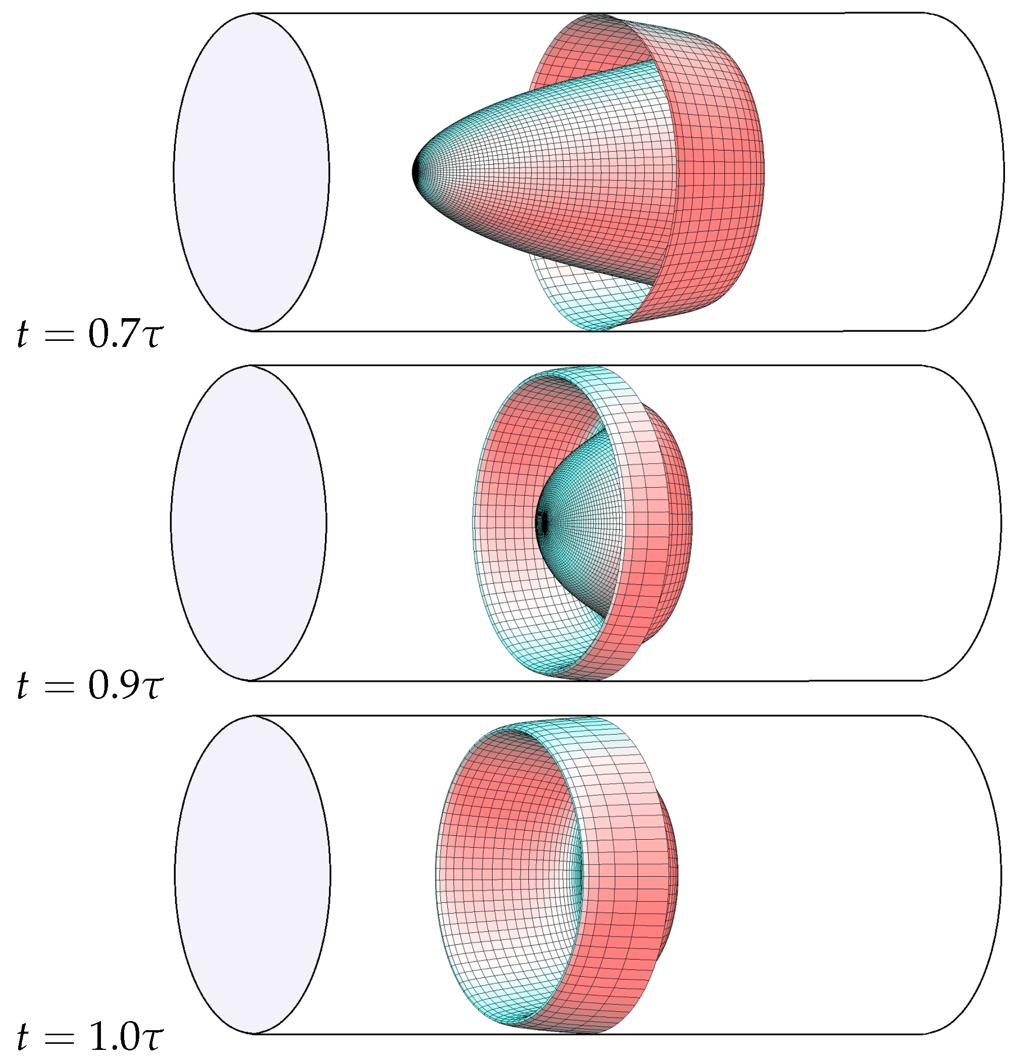
Figure 4 illustrates spatial velocity diagrams of the base flow at different times within one half-period of vibrations. A physical mechanism triggering the convection here is the thermovibrational one. The core of the pipe is heated better, and its density reduces. Cooler near-wall sublayers become denser. This is how a non-homogeneous stratification of density orthogonal to the cylinder axis is developed. Upon overlapping with the external inertial field, the system responds immediately by an unequal shift in the laminar sublayers. With condition (
47), this results in a non-trivial dynamics of the velocity diagram in time. For example, the strong warm flow in a positive direction along the
z-axis is observed at
(
Figure 4). It is surprising, but cold fluid near the cylinder walls moves in the same direction (
Figure 4,
). To balance these flows, the reverse fluid flow develops in the intermediate zone between the axis and the walls.


