A Theoretical Investigation of Flow Topologies in Bubble- and Droplet-Affected Flows

Abstract

A local flow topology analysis was conducted for laminar particle-affected flows. Based on the invariants of the velocity gradient tensor, all possible flow structures can be categorized into two focal and two nodal topologies for incompressible flows. The underlying field descriptions for bubble- and droplet-affected flows in the creeping flow regime were determined analytically for two different boundary conditions. A nodal-to-focal-to-nodal transition can be observed in both phases and the focal topologies are predominant in the interior phase. It was also found that the topology distribution in the interior phase is independent of the dynamic viscosity ratio and the boundary conditions, which is not the case in the exterior phase. The focal region in the exterior phase extends to infinity for the far-field boundary condition, whereas it is bounded to a tire-like zone attached to the bubble or droplet for the near-field boundary condition. Furthermore, the existence of a narrow band of intermediate nodal topologies was demonstrated analytically, which raises the question on the origin of this behavior. To complement the findings about the flow topology classification, the strengths of the underlying vorticity and invariant fields are discussed, including their dependency on the considered phase and boundary condition.

1. Introduction

Bubble- and droplet-laden flows play an essential role in many technical applications, e.g., for chemical reactors or safety installations in the process industry. To improve the fundamental understanding of particle-affected flows, this paper contributes a local flow topology analysis based on the analytical creeping flow solutions of Hadamard and Rybczynski [1] and Satapathy and Smith [2].

The topology classification follows the pioneering work of Chong et al. [3], Perry and Chong [4]. Using the invariants of the velocity gradient tensor, all possible small-scale flow structures can be categorized into two nodal and two focal topologies for incompressible flows. To analyze the different manifestation of coherent structures, the methodology has been applied to a variety of direct numerical simulation databases on wall-bounded shear flows [5], homogeneous isotropic turbulence [6] and compressible reactive flows [7]. Potential further analysis steps were demonstrated by Dopazo et al. [8], who studied the connection between local flow topologies and local geometry of iso-surfaces of an inert, dynamically passive scalar. Mixing characteristics were characterized in terms of principal curvatures or mean and Gauss curvatures.

Recently, Hasslberger et al. [9,10] compared the topology behavior in laminar and turbulent bubbly flows and revealed striking similarities—mainly the nodal-to-focal-to-nodal transition in main flow direction and the dominance of focal topologies in the gaseous interior phase. The briefly discussed laminar case in the work of Hasslberger et al. [9,10] was investigated in a semi-analytical manner, i.e., the velocity field was obtained from the analytical solution of Hadamard and Rybczynski [1] but the invariants calculation and the topology classification were conducted by means of a numerical tool. Elimination of numerical errors requires the fully analytical reinvestigation of the problem.

In this respect, the main objectives of this study were:

• to demonstrate that the topology distribution in the interior phase is independent of the dynamic viscosity ratio and the boundary conditions applied in the exterior phase;
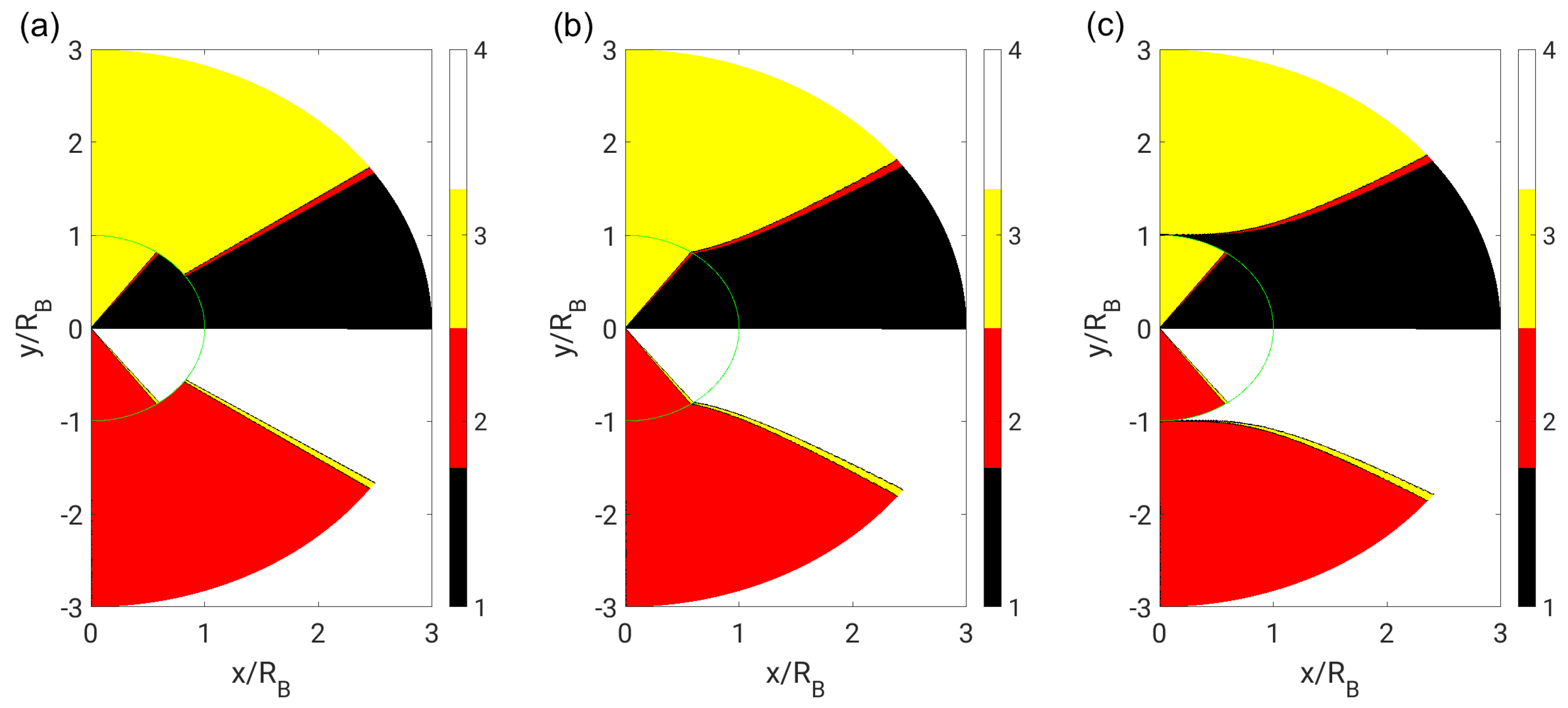
• to check upon the existence of a narrow band of intermediate nodal topologies;
• to derive explicit mathematical expressions for all topology borders in both phases;
• to calculate the universal topology volume fractions in the interior phase; and
• to provide an analytical reference solution for the purpose of numerical topology code validation.

It turns out that several flow features of significantly more complex turbulent flows (according to earlier investigations) can be readily explained by looking at the much simpler analytical creeping flow solution. In this regard, the present paper represents an important reference for particles and particle swarms in turbulent flows. This study might also inspire the modeling of particle-flow interaction when this interaction is not explicitly resolved in numerical simulations, e.g., in the Euler–Lagrange context.

2. Mathematical Description

2.1. Invariants of the Velocity Gradient Tensor and Flow Topologies

According to the authors of [3,4], the invariants of the velocity gradient tensor give rise to a set of local flow topologies, classifying arbitrary complex flows into canonical flow types. The velocity gradient tensor is given by

$$A\equiv \nabla \otimes \mathit{u},$$

(1)

where $\mathit{u}=u_r·{\widehat{e}}_r+u_{\theta }·{\widehat{e}}_{\theta }$ denotes the velocity field, ⊗ the dyadic product and ∇ the Nabla operator in spherical coordinates:

$$\nabla \equiv {\widehat{e}}_r\frac{\partial }{\partial r}+{\widehat{e}}_{\theta }\frac{1}{r}\frac{\partial }{\partial \theta }+{\widehat{e}}_{\phi }\frac{1}{rsin\theta }\frac{\partial }{\partial \phi }.$$

(2)

Since the velocity fields are assumed to be axisymmetric here ($\partial /\partial \phi =0$ and $u_{\phi }=0$), only the radial $u_r$ and circumferential component $u_{\theta }$ have to be considered. Thus, the velocity gradient tensor reduces to

$$\begin{array}{c}\hfill A=\frac{\partial u_r}{\partial r}\left({\widehat{e}}_r\otimes {\widehat{e}}_r\right)+\frac{1}{r}\left(u_r+\frac{\partial u_{\theta }}{\partial \theta }\right)\left({\widehat{e}}_{\theta }\otimes {\widehat{e}}_{\theta }\right)+\frac{1}{r}\left(u_r+\frac{u_{\theta }cos\theta }{sin\theta }\right)\left({\widehat{e}}_{\phi }\otimes {\widehat{e}}_{\phi }\right)\\ \hfill +\frac{1}{r}\left(\frac{\partial u_r}{\partial \theta }-u_{\theta }\right)\left({\widehat{e}}_r\otimes {\widehat{e}}_{\theta }\right)+\frac{\partial u_{\theta }}{\partial r}\left({\widehat{e}}_{\theta }\otimes {\widehat{e}}_r\right).\end{array}$$

(3)

The characteristic polynomial ${\lambda }^3+P{\lambda }^2+Q\lambda +R=0$ can be assigned to the tensor A, with $\lambda$ being its eigenvalues and $P,Q,R$ being its first, second and third invariants:

$$\begin{array}{ccc}\hfill P& \equiv & -\mathrm{tr}\left(A\right)\hfill \\ & =& 0,\hfill \\ \hfill Q& \equiv & \frac{1}{2}\left(\mathrm{tr}{\left(A\right)}^2-\mathrm{tr}\left(A^2\right)\right)\hfill \\ & =& -\frac{1}{2}\left[{\left(\frac{\partial u_r}{\partial r}\right)}^2+\frac{1}{r^2}{\left(u_r+\frac{u_{\theta }cos\theta }{sin\theta }\right)}^2+\frac{1}{r^2}{\left(u_r+\frac{\partial u_{\theta }}{\partial \theta }\right)}^2+\frac{2}{r}\frac{\partial u_{\theta }}{\partial r}\left(\frac{\partial u_r}{\partial \theta }-u_{\theta }\right)\right],\hfill \\ \hfill R& \equiv & -\det \left(A\right)\hfill \\ & =& \frac{1}{r^2}\left(u_r+\frac{u_{\theta }cos\theta }{sin\theta }\right)\left[\frac{\partial u_{\theta }}{\partial r}\left(\frac{\partial u_r}{\partial \theta }-u_{\theta }\right)-\frac{\partial u_r}{\partial r}\left(\frac{\partial u_{\theta }}{\partial \theta }+u_r\right)\right].\hfill \end{array}$$

(4)

Owing to the incompressibility of the fluid, i.e., $P=-\nabla ·\mathit{u}=0$, the $Q-R$ phase-space is subdivided into two focal topologies (S1 and S4) and two nodal topologies (S2 and S3). The boundaries separating the different regions are given by $R_2=0$, $R_{1a}=-2/\sqrt{27}\sqrt{-Q^3}$ and $R_{1b}=2/\sqrt{27}\sqrt{-Q^3}$, corresponding to the states where the characteristic equation’s discriminant $D=(27R^2+4Q^3)/108$ is zero. Both the topology borders $R_{1a}$, $R_{1b}$ and $R_2$ in the $Q-R$ phase-space, and a graphical representation of topologies S1–S4, are shown in Figure 1. Splitting up the tensor A into its symmetric and anti-symmetric part, it can further be demonstrated that $Q<0$ is indicative of strain-dominated regions and $Q>0$ is indicative of vorticity-dominated regions (cf., e.g., [10]).

2.2. Stream Function Ansatz

In the following, the flow inside and around rigid spherical bubbles or droplets is investigated. Using the creeping flow assumption (Reynolds number $Re\ll 1$), it can be derived from the basic equations of motion that the stream function $\psi (r,\theta )$, depending only on radius r and inclination $\theta$, must satisfy the bi-Laplacian

$${\nabla }^2{\nabla }^2\psi ={\left[\frac{{\partial }^2}{\partial r^2}+\frac{sin\theta }{r^2}\frac{\partial }{\partial \theta }\left(\frac{1}{sin\theta }\frac{\partial }{\partial \theta }\right)\right]}^2\psi =0.$$

(5)

Testing of trial functions $r^n{sin}^2\theta$ suggests that the general solution is of the form

$$\psi =\left(\frac{A}{r}+Br+C{r}^2+D{r}^4\right){sin}^2\theta ,$$

(6)

with the a priori unknown constants $A,B,C,D$—separately for each phase. Index G represents the interior phase, i.e., the gaseous phase for bubbles, and index L represents the exterior phase, i.e., the liquid phase for bubbles (and vice versa for droplets). To avoid singular behavior at the bubble or droplet center ($r=0$), $A_G=B_G=0$ is required in any case (cf. Equation (13)). At the phase interface ($r=r_B$), the continuity of normal velocity

$$u_{Gr}=u_{Lr},$$

(7)

tangential velocity

$$u_{G\theta }=u_{L\theta },$$

(8)

normal stress

$$-p_G+2{\mu }_G\frac{\partial u_{Gr}}{\partial r}=-p_L+2{\mu }_L\frac{\partial u_{Lr}}{\partial r},$$

(9)

and shear stress

$${\mu }_G\left(r\frac{\partial u_{G\theta }}{\partial r}-u_{G\theta }+\frac{\partial u_{Gr}}{\partial \theta }\right)={\mu }_L\left(r\frac{\partial u_{L\theta }}{\partial r}-u_{L\theta }+\frac{\partial u_{Lr}}{\partial \theta }\right)$$

(10)

are assumed.

Using the general relationships

$$u_r=\frac{1}{r^{2}sin\theta }\frac{\partial \psi }{\partial \theta }$$

(11)

and

$$u_{\theta }=-\frac{1}{rsin\theta }\frac{\partial \psi }{\partial r},$$

(12)

the velocity components can be deduced as

$$\begin{array}{ccc}\hfill u_{Gr}& =& 2cos\theta (C_G+D_G{r}^2),\hfill \\ \hfill u_{G\theta }& =& -2sin\theta (C_G+2D_G{r}^2),\hfill \\ \hfill u_{Lr}& =& 2cos\theta \left(\frac{A_L}{r^3}+\frac{B_L}{r}+C_L+D_L{r}^2\right),\hfill \\ \hfill u_{L\theta }& =& sin\theta \left(\frac{A_L}{r^3}-\frac{B_L}{r}-2C_L-4D_L{r}^2\right),\hfill \end{array}$$

(13)

with the corresponding partial derivatives

$$\begin{array}{ccc}\hfill \frac{\partial u_{Gr}}{\partial r}& =& 4D_{G}rcos\theta ,\hfill \\ \hfill \frac{\partial u_{Gr}}{\partial \theta }& =& -2sin\theta (C_G+D_G{r}^2),\hfill \\ \hfill \frac{\partial u_{G\theta }}{\partial r}& =& -8D_{G}rsin\theta ,\hfill \\ \hfill \frac{\partial u_{G\theta }}{\partial \theta }& =& -2cos(C_G+2D_G{r}^2)\hfill \end{array}$$

(14)

for the interior phase and

$$\begin{array}{ccc}\hfill \frac{\partial u_{Lr}}{\partial r}& =& 2cos\theta \left(-\frac{3A_L}{r^4}-\frac{B_L}{r^2}+2D_{L}r\right),\hfill \\ \hfill \frac{\partial u_{Lr}}{\partial \theta }& =& -2sin\theta \left(\frac{A_L}{r^3}+\frac{B_L}{r}+C_L+D_L{r}^2\right),\hfill \\ \hfill \frac{\partial u_{L\theta }}{\partial r}& =& sin\theta \left(-\frac{3A_L}{r^4}+\frac{B_L}{r^2}-8D_{L}r\right),\hfill \\ \hfill \frac{\partial u_{L\theta }}{\partial \theta }& =& cos\theta \left(\frac{A_L}{r^3}-\frac{B_L}{r}-2C_L-4D_L{r}^2\right)\hfill \end{array}$$

(15)

for the exterior phase.

On that basis, the second and third invariants (Equation (4)) of both phases can be expressed as

$$\begin{array}{ccc}\hfill Q_G& =& 4D_G^2{r}^2\left(4{sin}^2\theta -3{cos}^2\theta \right),\hfill \\ \hfill R_G& =& 16D_G^3{r}^{3}cos\theta \left(2{sin}^2\theta -{cos}^2\theta \right),\hfill \\ \hfill Q_L& =& -3{cos}^2\theta {\left(\frac{3A_L}{r^4}+\frac{B_L}{r^2}-2D_{L}r\right)}^2\hfill \\ & & +{sin}^2\theta \left(\frac{-3A_L}{r^4}+\frac{B_L}{r^2}-8D_{L}r\right)\left(\frac{3A_L}{r^4}+\frac{B_L}{r^2}-2D_{L}r\right),\hfill \\ \hfill R_L& =& 2{cos}^3\theta \frac{1}{r^3}{\left(\frac{3A_L}{r^3}+\frac{B_L}{r}-2D_L{r}^2\right)}^3\hfill \\ & & -{sin}^2\theta cos\theta \frac{1}{r^2}\left(\frac{-3A_L}{r^4}+\frac{B_L}{r^2}-8D_{L}r\right){\left(\frac{3A_L}{r^3}+\frac{B_L}{r}-2D_L{r}^2\right)}^2.\hfill \end{array}$$

(16)

2.3. Vorticity Field

The vorticity, as defined by

$$\omega \equiv \nabla \times \mathit{u},$$

(17)

is a fundamental quantity to describe vortex-affected flows. As such, it is closely related to the topology classification, as indicated in Section 2.1. In spherical coordinates, the vorticity is given by

$$\begin{array}{c}\hfill \omega =\frac{1}{rsin\theta }\left[\frac{\partial }{\partial \theta }(u_{\phi }sin\theta )-\frac{\partial u_{\theta }}{\partial \phi }\right]{\widehat{e}}_r+\frac{1}{r}\left[\frac{1}{sin\theta }\frac{\partial u_r}{\partial \phi }-\frac{\partial }{\partial r}\left(r{u}_{\phi }\right)\right]{\widehat{e}}_{\theta }+\\ \hfill \frac{1}{r}\left[\frac{\partial }{\partial r}\left(r{u}_{\theta }\right)-\frac{\partial u_r}{\partial \theta }\right]{\widehat{e}}_{\phi }.\end{array}$$

(18)

In the axisymmetric case characterized by $\partial /\partial \phi =0$ and $u_{\phi }=0$, the vorticity reduces to

$$\omega =\frac{1}{r}\left[\frac{\partial }{\partial r}\left(r{u}_{\theta }\right)-\frac{\partial u_r}{\partial \theta }\right]{\widehat{e}}_{\phi },$$

(19)

specifically to

$${\omega }_G=-10D_{G}rsin\theta {\widehat{e}}_{\phi }$$

(20)

for the interior phase and

$${\omega }_L=2sin\theta \left(\frac{B_L}{r^2}-5D_{L}r\right){\widehat{e}}_{\phi }$$

(21)

for the exterior phase. The ratio of non-zero vorticity components at the interface ($r=r_B$) can then be calculated as

$$\frac{{\omega }_G}{{\omega }_L}=-5\frac{D_G{r}_B}{\frac{B_L}{r_B^2}-5D_L{r}_B},$$

(22)

which does not depend on inclination $\theta$. As shown in the following, the vorticity field is generally discontinuous at the interface, except for identical dynamic viscosities in both phases, i.e., $\xi ={\mu }_G/{\mu }_L=1$.

2.4. Far-Field Boundary Conditions

The analytical solution of Hadamard and Rybczynski [1] is based on the far-field boundary conditions

$$u_r(r\to \infty )=u_{0}cos\theta ,u_{\theta }(r\to \infty )=-u_{0}sin\theta ,$$

(23)

where $u_0$ is the velocity of the bubble or droplet relative to the unperturbed surrounding flow. In this case, the constants of the stream function, Equation (6), are specified as

$$\begin{array}{ccc}\hfill A_L& =& \frac{u_0}{4}{r}_B^3\frac{\xi }{1+\xi },\hfill \\ \hfill B_L& =& -\frac{u_0}{4}{r}_B\frac{2+3\xi }{1+\xi },\hfill \\ \hfill C_L& =& \frac{u_0}{2},\hfill \\ \hfill D_L& =& 0,\hfill \\ \hfill C_G& =& -\frac{u_0}{4}\frac{1}{1+\xi },\hfill \\ \hfill D_G& =& \frac{u_0}{4}\frac{1}{r_B^2}\frac{1}{1+\xi }.\hfill \end{array}$$

(24)

The dynamic viscosity ratio of both phases is denoted as $\xi ={\mu }_G/{\mu }_L$ and the radius of the bubble or droplet as $r_B$. Corresponding to the fluid properties of gaseous air and liquid water, $\xi$-values of 0.0182, 1.0 and 54.9583 are referred to as the bubble, neutral and droplet cases, respectively. In the bubble case with far-field boundary conditions, Figure 2 depicts the streamlines as well as radial and circumferential velocity components in both phases.

2.5. Near-Field Boundary Conditions

The analytical solution of Satapathy and Smith [2] generally follows the same procedure. However, instead of using far-field boundary conditions, the boundary conditions are imposed at a particular distance from the origin:

$$u_r(r=r_W)=u_{0}cos\theta ,u_{\theta }(r=r_W)=-u_{0}sin\theta .$$

(25)

These boundary conditions are supposed to enforce a constant-velocity parallel flow at $r=r_W$ and can be interpreted as a symmetry condition between neighboring particles (in swarms) or a side wall oriented in mean flow direction. Thus, they are more appropriate to reflect the bubble or droplet behavior in confined flow domains than the usage of far-field boundary conditions. Note that the given solution is meaningless for $r>r_W$.

It is worth mentioning that the constants in the original publication of Satapathy and Smith [2] are incorrectly printed. Here, only the corrected set of constants (also explicitly including the dependency on $u_0$ and $r_B$) is presented:

$$\begin{array}{ccc}\hfill A_L& =& u_0\frac{r_W^3}{\alpha }\left[\frac{1}{\xi }+{\left(\frac{r_W}{r_B}\right)}^3-1\right],\hfill \\ \hfill B_L& =& -u_0\frac{r_W}{\alpha }\left[-3+\frac{3}{\xi }+3{\left(\frac{r_W}{r_B}\right)}^5+\frac{2}{\xi }{\left(\frac{r_W}{r_B}\right)}^5\right],\hfill \\ \hfill C_L& =& u_0\frac{r_W}{r_B}\frac{1}{2\alpha }\left[-9+5{\left(\frac{r_W}{r_B}\right)}^2+4{\left(\frac{r_W}{r_B}\right)}^5+\frac{1}{\xi }\left(6+4{\left(\frac{r_W}{r_B}\right)}^5\right)\right],\hfill \\ \hfill D_L& =& u_0\frac{1}{r_B^2}\frac{1}{2\alpha }\left[3\frac{r_W}{r_B}-{\left(\frac{r_W}{r_B}\right)}^3\left(3+\frac{2}{\xi }\right)\right],\hfill \\ \hfill D_G& =& \frac{1}{\xi }\left[\frac{A_L}{r_B^5}+D_L\right],\hfill \\ \hfill C_G& =& -D_G{r}_B^2,\hfill \end{array}$$

(26)

using the abbreviation

$$\begin{array}{c}\hfill \alpha ={\left(\frac{r_W}{r_B}-1\right)}^3[-4-3\frac{r_W}{r_B}+3{\left(\frac{r_W}{r_B}\right)}^2+4{\left(\frac{r_W}{r_B}\right)}^3\\ \hfill +\frac{1}{\xi }\left(4+6\frac{r_W}{r_B}+6{\left(\frac{r_W}{r_B}\right)}^2+4{\left(\frac{r_W}{r_B}\right)}^3\right)].\end{array}$$

(27)

In the bubble case with near-field boundary conditions ($r_W=3r_B$), Figure 3 depicts the streamlines as well as radial and circumferential velocity components in both phases. The comparison with far-field boundary conditions (Figure 2) reveals a qualitatively similar behavior, especially regarding the torus-like recirculation in the interior phase. Slight differences can be observed regarding the deflection of streamlines in the exterior phase. Furthermore, the near-field boundary conditions result in a maximum of velocity magnitude above $u_0$ (at $\theta ={90}^{\circ }$, in the region $r_B<r<r_W$), which is due to continuity reasons. Velocity magnitudes exceeding $u_0$ do not occur in the solution with far-field boundary conditions.

3. Results and Discussion

In all of the presented field plots, the green line indicates the phase interface. Owing to the symmetry of the problem, only half of the fields is visualized each. Without any loss of generality, $u_0=1\mathrm{m}/\mathrm{s}$ is chosen. As depicted in the streamline plots in Figure 2 and Figure 3, the mean flow direction in the exterior phase is from bottom to top.

3.1. Vorticity Field

A comparison of the vorticity field $\omega$ (Equation (19)) based on both boundary conditions is presented in Figure 4. Note that only the plane-normal component is unequal to zero. In the interior phase, the general shape of the solution is the same in both cases. Quantitative differences are determined by $r_W$, i.e., the radius at which the near-field boundary condition is imposed. The vorticity jump at the interface is given by Equation (22), and the phase in which the maximum vorticity magnitude appears, is eventually determined by the dynamic viscosity ratio $\xi$. In the bubble case shown here, the vorticity peak can be found in the gaseous phase.

In the exterior phase, the solution is not even qualitatively the same. In both cases and in both phases, the vorticity is zero for $\theta =0^{\circ }$ as well as $\theta ={180}^{\circ }$ and it peaks at $\theta ={90}^{\circ }$. However, the vorticity steadily decays to zero for $r\to \infty$ with far-field boundary conditions. According to Equation (21), the zero-vorticity iso-contour in the exterior phase (black line in Figure 4) is given by $r=\sqrt[3]{B_L/\left(5D_L\right)}$, which is smaller than $r_W$ for near-field boundary conditions. Note that $D_L=0$ for far-field boundary conditions in contrast. It might be questioned whether the imposed near-field boundary condition (Equation (25)) is an adequate choice. The idea of a constant parallel flow for $r\ge r_W$ implies vanishing velocity gradients, which is not satisfied at $r=r_W$. The differences in the vorticity field are also reflected in the topology classification discussed subsequently.

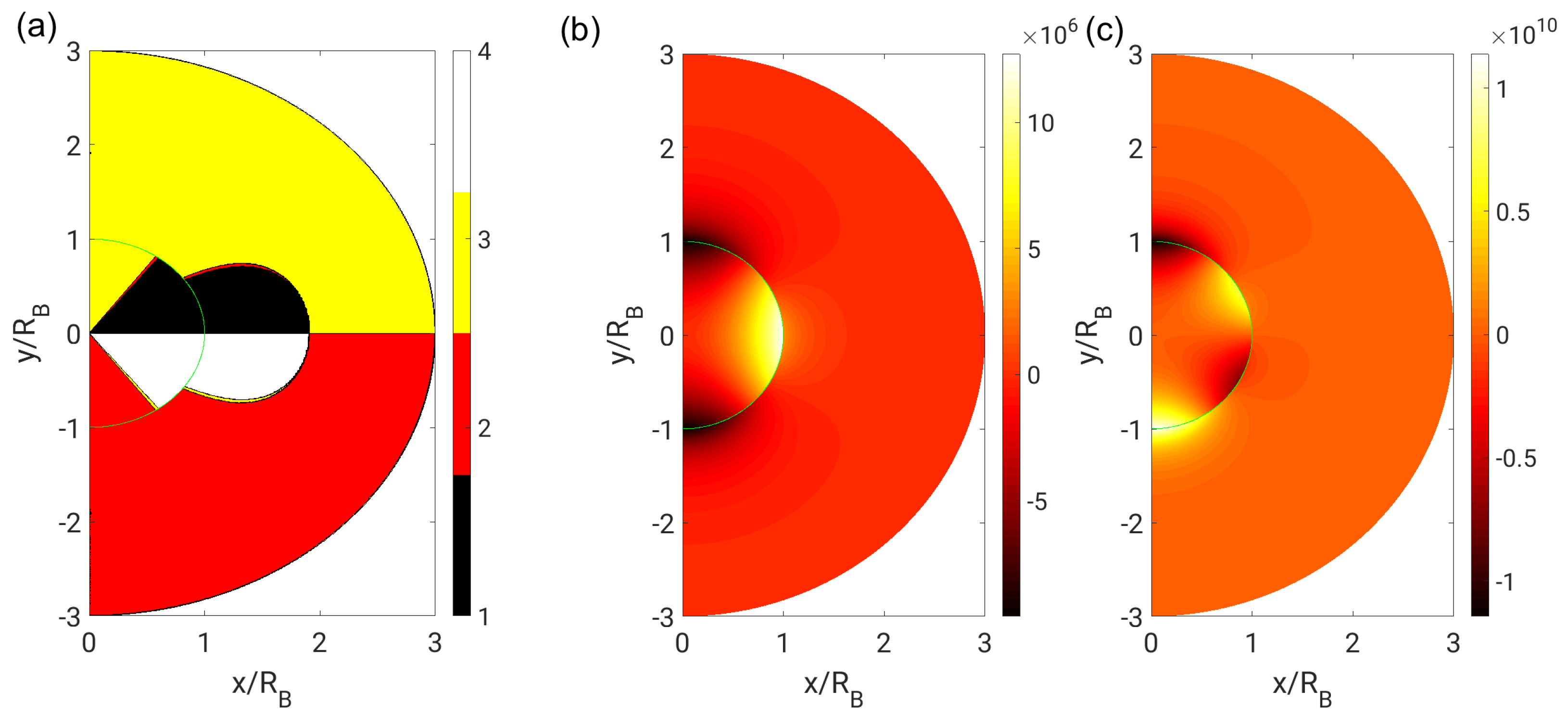
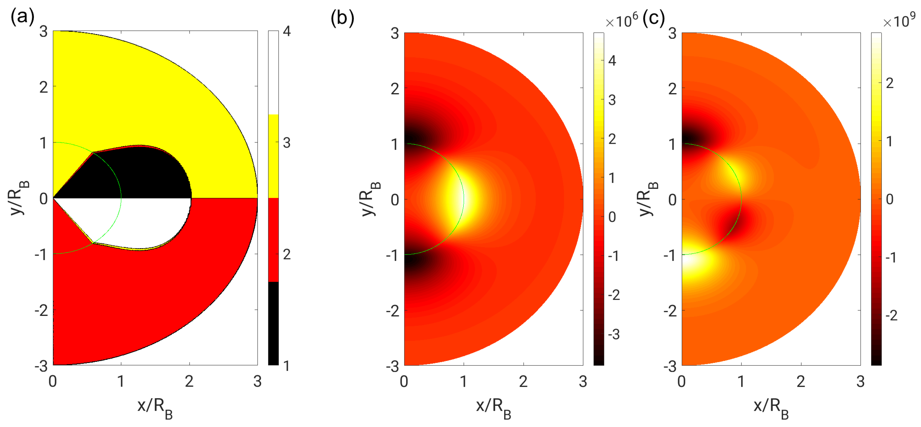
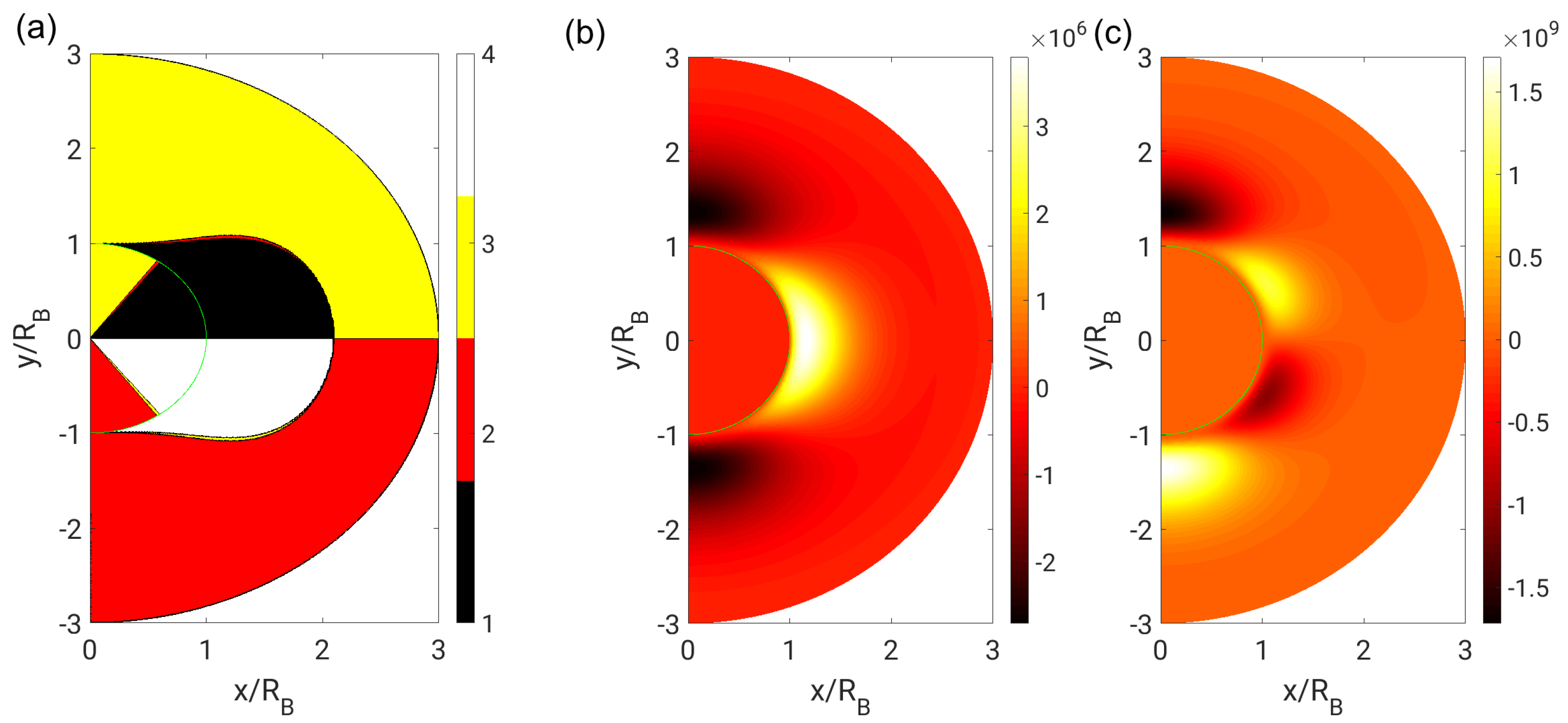
3.2. Invariants and Flow Topologies

As introduced in Section 2.1, the result of the flow topology classification with far-field boundary conditions is shown in Figure 5, Figure 6 and Figure 7 for different dynamic viscosity ratios. In addition, the corresponding invariant fields (Equation (4)) are plotted since these also contain information on the strength of the underlying fields. First, it can be observed that the focal topologies (S1 and S4), according to their vortical nature, prevail in the high vorticity regions where $Q>0$. Secondly, the topology behavior at the phase interface is continuous in the neutral case ($\xi =1$), whereas a discontinuous behavior can be observed for the bubble case ($\xi =0.0182$) and the droplet case ($\xi =54.9583$). Accordingly, the second invariant Q and the third invariant R exhibit a continuous or discontinuous behavior depending on the case.

Following the flow pathlines (which coincide with the streamlines for steady flows, as depicted in Figure 2), the sequence of the adopted flow topologies (nodal-to-focal-to-nodal transition) is generally the same in all cases. Regarding the distribution of nodal topologies, mainly S2 can be found in the upstream and S3 in the downstream part of the domain, respectively. However, a close inspection of the topology fields reveals a narrow band of intermediate nodal topologies (switching between S2 and S3) in both phases. It may be questioned whether this behavior is a consequence of the particular stream function ansatz (Equation (6)) or whether it is strictly necessary due to physical reasons. The existence of theses intermediate topologies cannot be explained by numerical inaccuracies. In fact, it can be shown analytically that the S2–S3 transition in the interior phase is specified by the constraint $R_G=0$:

$$cos{\theta }_{2-3,G}\left({cos}^2{\theta }_{2-3,G}-2{sin}^2{\theta }_{2-3,G}\right)=0,$$

(28)

which is satisfied at

$${\theta }_{2-3,G}=\arctan \left(\frac{1}{\sqrt{2}}\right)=\arccos \left(\sqrt{\frac{2}{3}}\right)\approx 35.26°,$$

(29)

and ${180}^{\circ }-{\theta }_{2-3,G}$, respectively. In contrast, the S1–S2 transition is specified by the constraint $R_G=R_{1bG}$:

$$-\frac{1}{4}cos{\theta }_{1-2,G}\left({cos}^2{\theta }_{1-2,G}-2{sin}^2{\theta }_{1-2,G}\right)=\frac{2}{\sqrt{27}}{\left(\frac{3}{4}{cos}^2{\theta }_{1-2,G}-{sin}^2{\theta }_{1-2,G}\right)}^{\frac{3}{2}},$$

(30)

which is satisfied at

$${\theta }_{1-2,G}=\arctan \left(\frac{3}{4}\right)=\arccos \left(\frac{4}{5}\right)\approx 36.87°.$$

(31)

For symmetry reasons, the S3–S4 transition occurs at ${\theta }_{3-4,G}={180}^{\circ }-{\theta }_{1-2,G}$. Remarkably, the topology borders in the interior phase are straight lines, which depend on neither the radial coordinate r nor the dynamic viscosity ratio $\xi$. The constant topology volume fractions can thus be calculated to be

$$\frac{V_{S2}+V_{S3}}{V_{total}}=\frac{2·2/3\pi r_B^2·r_B(1-cos{\theta }_{1-2,G})}{4/3\pi r_B^3}=1-cos{\theta }_{1-2,G}=20\%$$

(32)

for nodal topologies (S2 + S3), and consequently 80% for focal topologies (S1 + S4). Exactly the same values were theoretically predicted by Hasslberger et al. [11], but with a very different approach.

In the exterior phase, the S2–S3 transition is specified by the constraint $R_L=0$:

$$\begin{array}{cc}& 2{cos}^3{\theta }_{2-3,L}{\left(\frac{3A_L}{r^4}+\frac{B_L}{r^2}-2D_{L}r\right)}^3\hfill \\ \hfill =& {sin}^2{\theta }_{2-3,L}cos{\theta }_{2-3,L}\left(-\frac{3A_L}{r^4}+\frac{B_L}{r^2}-8D_{L}r\right){\left(\frac{3A_L}{r^4}+\frac{B_L}{r^2}-2D_{L}r\right)}^2,\hfill \end{array}$$

(33)

which is satisfied at

$${\theta }_{2-3,L}\left(r\right)=\arctan \left(\sqrt{\frac{4D_L{r}^5-2B_L{r}^2-6A_L}{8D_L{r}^5-B_L{r}^2+3A_L}}\right),$$

(34)

and ${180}^{\circ }-{\theta }_{2-3,L}$, respectively. The S1–S2 transition is specified by the constraint $R_L=R_{1bL}$:

$$\begin{array}{cc}& 2{cos}^3{\theta }_{1-2,L}{\left(\frac{3A_L}{r^4}+\frac{B_L}{r^2}-2D_{L}r\right)}^3\hfill \\ & -{sin}^2{\theta }_{1-2,L}cos{\theta }_{1-2,L}\left(-\frac{3A_L}{r^4}+\frac{B_L}{r^2}-8D_{L}r\right){\left(\frac{3A_L}{r^4}+\frac{B_L}{r^2}-2D_{L}r\right)}^2\hfill \\ \hfill =& \frac{2}{\sqrt{27}}[3{cos}^2{\theta }_{1-2,L}{\left(\frac{3A_L}{r^4}+\frac{B_L}{r^2}-2D_{L}r\right)}^2\hfill \\ & -{sin}^2{\theta }_{1-2,L}\left(-\frac{3A_L}{r^4}+\frac{B_L}{r^2}-8D_{L}r\right)\left(\frac{3A_L}{r^4}+\frac{B_L}{r^2}-2D_{L}r\right){]}^{\frac{3}{2}},\hfill \end{array}$$

(35)

which is satisfied at

$${\theta }_{1-2,L}\left(r\right)=\arccos \left(2\sqrt{\frac{8D_L{r}^5-B_L{r}^2+3A_L}{50D_L{r}^5-13B_L{r}^2-15A_L}}\right).$$

(36)

Again, for symmetry reasons, the S3–S4 transition occurs at ${\theta }_{3-4,L}={180}^{\circ }-{\theta }_{1-2,L}$. Equations (34) and (36) reveal that the topology borders in the exterior phase are generally curved and furthermore depend on the viscosity ratio. To determine the extent of the focal region in the exterior phase $r^{*}$ (a finite value only for near-field boundary conditions), ${\theta }_{1-2,L}\left(r^{*}\right)=\pi /2$, representing the horizontal line through the origin, can be inserted in Equation (36), which yields a fifth-order equation that can be solved numerically:

$$8D_L{\left(r^{*}\right)}^5-B_L{\left(r^{*}\right)}^2+3A_L=0.$$

(37)

Independent of the phase, the transition between focal topologies S1 and S4 occurs at ${\theta }_{1-4}={90}^{\circ }$.

The topology and invariant fields with near-field boundary conditions are shown in Figure 8, Figure 9 and Figure 10 for $r_W=3r_B$. To facilitate a direct comparison with far-field boundary conditions, the same range of dynamic viscosity ratios is investigated as in Figure 5, Figure 6 and Figure 7. In addition, in this case, the topology and invariant fields are continuous at the phase interface only if $\xi =1$. The topology distribution in the interior phase is identical for both types of boundary condition. The main difference concerns the shape of the focal region in the exterior phase. The focal region extends to the end of the domain (and probably to infinity) with far-field boundary conditions, whereas it is bounded to a tire-like zone around the bubble or droplet with near-field boundary conditions.

The functional relationships describing the topology borders are already given by Equations (29)–(36). It is worth noting that the topology distribution in the interior phase is identical for both boundary conditions since the stream function constants do not appear in Equations (29) and (31).

To check the universality of the findings, very small ($\xi ={10}^{-5}$) and very large ($\xi ={10}^5$) dynamic viscosity ratios were tested in addition to the water–air bubble ($\xi =0.0182$) and droplet case ($\xi =54.9583$). The topology fields are depicted in Figure 11 for far-field boundary conditions and in Figure 12 for near-field boundary conditions. It appears that the behavior for very small and very large dynamic viscosity ratios is not significantly different to the bubble and droplet case. For very small ratios and with far-field boundary conditions, the topology borders seem to approach straight lines even in the exterior phase. For very large ratios, the focal region in the exterior phase seems to completely enclose the interior phase for both boundary conditions. In general, differences in the topology field due to the boundary conditions increase with increasing distance from the bubble or droplet.

Finally, the influence of $r_W$, i.e., the radius where the near-field boundary condition is imposed, on the topology field was investigated in Figure 13. The behavior corresponding to $r_W=3r_B$ of the previously discussed cases was compared to an even smaller value of $r_W=1.5r_B$ and a much larger value of $r_W=100r_B$. As can be expected, the general shape of the solution is the same for a constant dynamic viscosity ratio ($\xi =1$ here). It is clear that the solution based on near-field boundary conditions approaches the solution based on far-field boundary conditions for very large values of $r_W$, i.e., when $r_W\to \infty$.

3.3. Phase-Space Projection

To obtain the scatter plots of the second invariant Q and the third invariant R, the solution was discretized by steps of $r_B/2000$ and $\pi /2000$ in r- and $\theta$-direction, respectively. The full range of data points is contained in Figure 14 and a magnified view close to the origin of the phase-space diagram is presented in Figure 15. The topology borders $R_{1a}$, $R_{1b}$ and $R_2$, as introduced in Section 2.1, are included as well. A high density of data points seems to occur near the origin of the phase-space diagram. It is interesting to note that direct transitions between all four topologies are possible via the origin. Furthermore, strong alignment of the points with the topology borders $R_{1a}$ and $R_{1b}$ can be found in the region representing nodal topologies S2 and S3. Even for highly irregular turbulent bubble flows, the same observation was made by Hasslberger et al. [10] by means of three-dimensional direct numerical simulations. The distribution of points is generally similar for both phases and both boundary conditions. It can be observed that the population in the phase-space diagram is also symmetric with respect to $R=0$, i.e., the volume fractions of nodal topologies S2 and S3 as well as focal topologies S1 and S4 are identical. However, the disparity of extreme values of Q and R is clearly different. In the bubble case shown here, the disparity of extreme values is larger in the interior, i.e., gaseous, phase. The disparity of extreme values is generally larger with near-field boundary conditions.

4. Concluding Remarks

A local flow topology analysis was conducted for laminar flows around a spherical bubble or droplet. The flow field was described by two analytical solutions, which differ in the boundary conditions. It was observed that the outer flow is essentially characterized by a diverging nodal flow field in front of the sphere, which converges after the flow obstacle. In between, focal topologies occur at the regions of simultaneous high streamline curvature and velocity magnitude, where the vorticity is also highest. The coupled inner flow is characterized by a torus-like recirculation and the focal topologies are predominant. It was demonstrated analytically that the topology distribution in the interior phase is independent of the dynamic viscosity ratio and the boundary conditions, whereas the topology distribution in the exterior phase depends on both these influencing factors. In particular, the focal region in the exterior phase extends to infinity for far-field boundary conditions, but it is bounded to a tire-like zone attached to the bubble or droplet for near-field boundary conditions.

The constant topology volume fractions in the interior phase can be calculated as 20% for nodal topologies (S2 + S3), and consequently 80% for focal topologies (S1 + S4). It is remarkable that these values match exactly the theoretical predictions reported earlier in the literature (using a very different approach than here).

An unintuitive discovery is the distinct existence of a very narrow band of intermediate nodal topologies such that the transition occurs between neighboring topologies in cyclic order, i.e., S1-S2-S3-S4-S1. In principle, topology changes could also happen across the origin of the Q-R phase-space in a different manner, and it is not clear whether the cyclic transition is a consequence of the particular stream function ansatz or due to physical reasons.

Although this analysis is limited to a creeping flow solution, a qualitatively similar behavior was observed in the literature for bubbles in a turbulent flow field. Hence, the results of this analysis might stimulate the modeling of the two-way coupling in the Euler–Lagrange context, when this interaction cannot be resolved explicitly.

References

- Sadhal, S.; Ayyaswamy, P.; Chung, J. Transport Phenomena with Drops and Bubbles; Springer Science and Business Media: New York, NY, USA, 2012. [Google Scholar]
- Satapathy, R.; Smith, W. The motion of single immiscible drops through a liquid. J. Fluid Mech. 1961, 10, 561–570. [Google Scholar] [CrossRef]
- Chong, M.; Perry, A.; Cantwell, B. A general classification of three-dimensional flow fields. Phys. Fluids A Fluid Dyn. 1990, 2, 765–777. [Google Scholar] [CrossRef]
- Perry, A.; Chong, M. A description of eddying motions and flow patterns using critical-point concepts. Ann. Rev. Fluid Mech. 1987, 19, 125–155. [Google Scholar] [CrossRef]
- Chong, M.; Soria, J.; Perry, A.; Chacin, J.; Cantwell, B.; Na, Y. Turbulence structures of wall-bounded shear flows found using DNS data. J. Fluid Mech. 1998, 357, 225–247. [Google Scholar] [CrossRef]
- Elsinga, G.; Marusic, I. Universal aspects of small-scale motions in turbulence. J. Fluid Mech. 2010, 662, 514–539. [Google Scholar] [CrossRef]
- Wacks, D.; Chakraborty, N.; Klein, M.; Arias, P.; Im, H. Flow topologies in different regimes of premixed turbulent combustion: A direct numerical simulation analysis. Phys. Rev. Fluids 2016, 1, 083401. [Google Scholar] [CrossRef]
- Dopazo, C.; Martín, J.; Hierro, J. Local geometry of isoscalar surfaces. Phys. Rev. E 2007, 76, 056316. [Google Scholar] [CrossRef] [PubMed]
- Hasslberger, J.; Klein, M.; Chakraborty, N. Local flow topology analysis applied to bubble-induced turbulence. In Proceedings of the 12th International ERCOFTAC Symposium on Engineering Turbulence Modelling and Measurements, Montpellier, France, 26–28 September 2018. [Google Scholar]
- Hasslberger, J.; Klein, M.; Chakraborty, N. Flow topologies in bubble-induced turbulence: a direct numerical simulation analysis. J. Fluid Mech. 2018, 857, 270–290. [Google Scholar] [CrossRef]
- Hasslberger, J.; Ketterl, S.; Klein, M.; Chakraborty, N. Flow topologies in primary atomization of liquid jets: A direct numerical simulation analysis. J. Fluid Mech. 2019, 859, 819–838. [Google Scholar] [CrossRef]
© 2019 by the authors. Licensee MDPI, Basel, Switzerland. This article is an open access article distributed under the terms and conditions of the Creative Commons Attribution (CC BY) license (http://creativecommons.org/licenses/by/4.0/).
Share and Cite
Hasslberger, J.; Marten, S.; Klein, M. A Theoretical Investigation of Flow Topologies in Bubble- and Droplet-Affected Flows. Fluids 2019, 4, 117. https://doi.org/10.3390/fluids4030117
Hasslberger J, Marten S, Klein M. A Theoretical Investigation of Flow Topologies in Bubble- and Droplet-Affected Flows. Fluids. 2019; 4(3):117. https://doi.org/10.3390/fluids4030117
Chicago/Turabian StyleHasslberger, Josef, Svenja Marten, and Markus Klein. 2019. "A Theoretical Investigation of Flow Topologies in Bubble- and Droplet-Affected Flows" Fluids 4, no. 3: 117. https://doi.org/10.3390/fluids4030117
APA StyleHasslberger, J., Marten, S., & Klein, M. (2019). A Theoretical Investigation of Flow Topologies in Bubble- and Droplet-Affected Flows. Fluids, 4(3), 117. https://doi.org/10.3390/fluids4030117