1. Introduction
Extreme wave, also known as freak wave or rogue wave, refers in oceanography to large water wave with crest-to-trough wave height
H exceeding twice the significant wave height
in the wave field, or with wave crest height
higher than
[
1]. In a Gaussian sea state, wave heights
H follow a Rayleigh distribution when the wave field is assumed to be narrow-banded. In such cases, large waves fulfilling the criteria
are not so unusual, occurring approximately once every 3000 waves. For instance, if the average wave period
s, it implies that the observer could probably encounter one of such waves in 12 h. What makes this particular field of research interesting is the fact that the extreme waves may occur not only in the energetic storm sea state but also in a calm sea state, making these waves outstanding and exceptional compared to the surrounding waves. These extreme waves are supposed to be very rare basing on Rayleigh distribution model, whereas they seem to have a larger occurrence in the real world, as suggested in the following scientific studies and reports [
2,
3,
4,
5].
The possible mechanisms of the formation of extreme waves are summarised and discussed in recent reviews [
6,
7]. One of the well-known mechanisms of the generation of freak waves is the so-called Benjamin–Feir (or modulational) instability [
8,
9], which is frequently studied within the framework of the nonlinear Schrödinger equation (NLS). The NLS equation can describe the evolution of the narrow-banded weakly nonlinear waves [
10,
11,
12,
13]. More recent reviews show that real sea states are more complex and one needs to consider three-dimensionality [
14], dissipation [
15,
16,
17] and breaking [
18] to achieve more accurate modeling of such wave fields. For constant water depth, the modulation instability of unidirectional waves should disappear with the relative water depth
(
k denotes the wave number and
h is the water depth) [
8,
19]. However, for the multidirectional sea states, this is no longer the case. The three-dimensionality not only affects the modulation instability but also the statistical parameters [
20,
21]; the sea states are either focusing or defocusing depending on the spreading angle. Although we are aware of the essential importance of short-crest waves, the topic of this paper is restricted to one horizontal propagation direction case since the uneven bottom effects on freak waves are not fully understood yet in such configuration. Recently, it has been emphasised that the formation of extreme waves is more related to the second/third-order non-resonant or bound harmonic waves than modulation instability, especially in the finite water depth case where the instabilities are further attenuated [
22].
The evidence of the link between a water depth transition and a higher probability of the occurrence of extreme waves has been shown both experimentally [
23,
24], and numerically [
25,
26,
27]. There are also studies dealing with extreme wave statistics in coastal areas with different shapes of variable bathymetry. Katsardi et al. (2013) [
28] conducted experimental tests with unidirectional waves propagating over mild bed slopes (1:100 and 1:250) including breaking zones, and made extensive comparisons of wave height distributions. Nonlinear transformation of irregular waves propagating over sloping bottoms (1:15, 1:30 and 1:45) is discussed using wavelet-based bicoherence in [
29]. Ma et al. (2014) [
30] studied spatial variations of skewness, kurtosis and groupiness factor for irregular waves over a bar (1:20) in shallow water. The obliquity effects on the statistical parameters are discussed in [
21] using 3D simulations with a High-Order Spectral (HOS) model.
In this context, the objectives of the present study were three-fold: (1) studying experimentally the statistical distribution of (extreme) wave heights considering variable bottom coastal conditions in a uni-directional water wave flume; (2) comparing the collected temporal wave profiles and corresponding statistical distributions with the results from two advanced numerical models; and (3) comparing the measured and simulated wave height distributions with a number of existing statistical models. Regarding Objective 1, the spatial evolution of unidirectional irregular sea states due to the presence of a constant bottom gradient was studied in the large scale facility of Tainan Hydraulics Laboratory (THL) in Taiwan. This large facility allowed us to investigate the full life cycle of extreme waves, from the generation to the degeneration. Several cases with different experimental conditions were tested, while one representative case was investigated for the validation of numerical nonlinear models. In addition to the overall evolution of the sea state, particular attention was paid to the sloping bottom zone as well as the two depth transition regions. Regarding Objective 2, two accurate numerical models were adopted to simulate the experiments, both based on the fully nonlinear potential flow theory: a higher-order Boussinesq-type model based on the model in [
31] and the highly nonlinear and dispersive model, whispers3D, using a spectral approximation of the potential in the vertical direction [
32,
33]. As shown below, the corresponding results indicate that the increase of the probability of occurrence of freak waves was clearly observed in experiments and well captured in the simulations, over a region where the water depth is relatively mildly varying. Both measured and simulated wave profiles were studied by using statistical, spectral and bispectral analysis. Finally, Objective 3 was devoted to the statistical distributions of measured and simulated wave heights comparing with six existing statistical distribution models.
The present article is structured as follows. In
Section 2, the experimental set-up and the tested sea state conditions are introduced. The mathematical models and their numerical implementations are presented in
Section 3. Several signal processing techniques are adopted to interpret the obtained data: from the measurements as well as the simulations, including spectral analysis (
Section 4), bispectral analysis (
Section 5), nonlinear wave parameters analysis (
Section 6), and statistical analysis of the wave height distribution (
Section 7). Conclusively, the main results are summarised in
Section 8.
2. Experimental Set-Up and Test Conditions
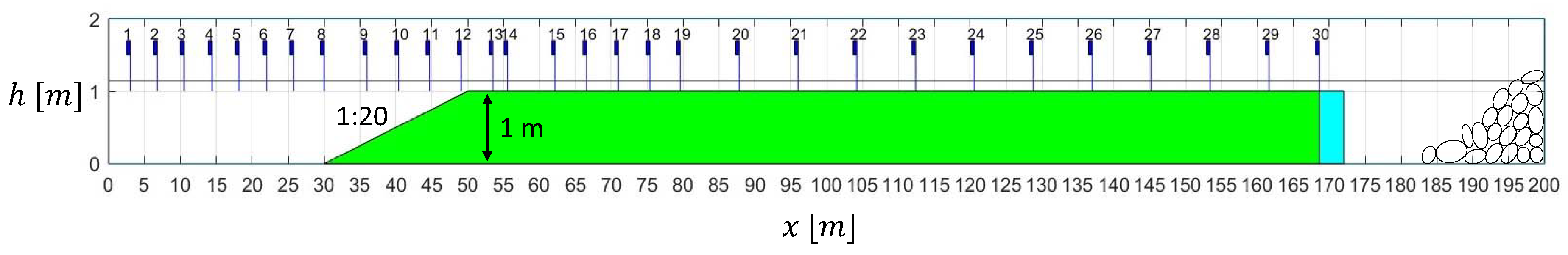
The experiments were conducted in the 2-D wave flume of THL at Tainan, Taiwan. The flume is 200 m long and 2 m wide. The waves were initially generated in the deeper region with depths of
m and
m. The bathymetry was decomposed into three parts: a 30 m long flat part, a 20 m long part with a constant slope of
and again a 120 m long flat bottom part. Waves were generated at
m by a piston-type wave-maker, which was also able to absorb part of the wave energy reflected by the uneven bottom or far-field rip-rap mound. The last 30 m part of the flume worked as an effective wave absorber including a deep water area and a mound of stones placed at the end of the flume. Over the flume length, 30 capacitance gauges were used to measure the wave elevation with a sampling frequency of 100 Hz. The locations of the wave gauges are shown in
Figure 1.
The first probe, located at m, was used as a reference for the input signal generated by the wavemaker, and then 7 additional wave probes were used to measure the wave evolution in the deeper area. Probes 9–12 were used to record the wave evolution over the slope. Several probes were distributed in the shallower region to observe the post-dynamics of extreme waves appearing around the end of the bottom slope.
Unidirectional irregular waves were generated using a linear superposition model using random initial phases and amplitudes as determined from a JONSWAP spectrum, given in Equation (
1). The experimental condition was controlled by four parameters: water depth
h, significant wave height
, peak frequency
and the peak enhancement factor
.
where
g denotes the gravitational acceleration;
denotes the adjustment factor to achieve the target
; and
denotes the spectral asymmetric parameter with respect to (w.r.t.) the spectral peak at
, with
when
and
when
. The spectrum was discretised using 16,384 = 2
14 frequency components over the range
to generate irregular sea states.
During the experimental campaign, more than 30 cases were tested, which were chosen based on the nonlinearity (wave steepness
, with
being the wave number corresponding to the peak wave period
) and the dispersion (w.r.t. the relative water depth
) in the deeper and shallower regions. The relative importance of these two effects was measured by the Ursell number
. For each test, the test duration lasted for
. Among all tests, the experimental results of three representative cases shown in
Table 1 have already been studied [
34].
Only Case 2 was selected and simulated in this study for the following reasons: (1) the sea state of Case 1 is almost Gaussian and the number of measured large waves is insufficient to do reliable statistical analysis; (2) in Cases 2 and 3, the relative water depth
is verified for the whole bottom profile, which means the effect of modulation instability can be ignored; and (3) Cases 2 and 3 show similar behaviour in both the statistical and spectral analyses. Case 2 is also preferred because fewer wave breaking events happened during the experiment, and they are not accounted for in the two numerical models. Regarding the wave parameters, one difference between the work of Trulsen et al. [
23] and the present work is that the nonlinearity of the waves in our case is significantly increased by the shoaling over the slope (note that
in our case is larger than
in the shallower side of Case 1 in [
23]) with the dispersion effects, i.e.,
and
being similar. Regarding the wave tank, our configuration was shorter in the deeper part but longer in the shallower part, also the slope is longer with the normalised length
(
denotes the length of slope) than in [
23] where
. Finally, a larger number of wave gauges were set in the flume to follow the wave evolution in space.
4. Data Processing: Spectral Analysis
Assuming that the free surface elevation is the sum of a large (infinite) number of statistically independent harmonic waves, each component having a random phase in and a constant positive amplitude, we operated with a Gaussian sea state and the statistical characteristics can be described through simple Fourier analysis. The spectral analysis was applied to both measured and simulated results. The simulated signals were resampled (by means of interpolation) to have the same sample points. A low-pass filter was applied to the measured signals to exclude the undesired high-frequency band which might be contaminated by the electronic noise of the wave probes. The time window where the analysis was carried out was translated for each wave gauge with the group velocity , which ensured that all analysed signals recorded at different positions roughly started from the same wave event. The spectra were estimated via Welch’s method. The overlapping factor was , with which the signals were separated into a number of segments. First, the Hann window was applied to each segment of signal (approximately 80 s), and then it was Fourier-transformed through -point fast Fourier transform (FFT), resulting in a high spectral resolution Hz.
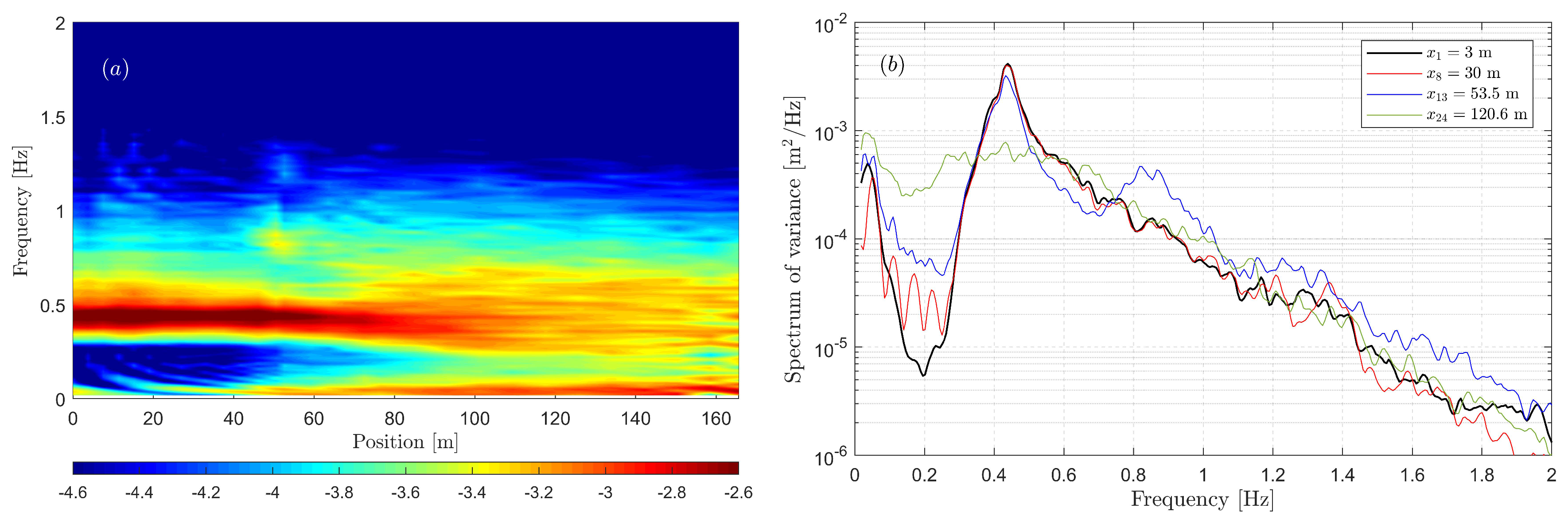
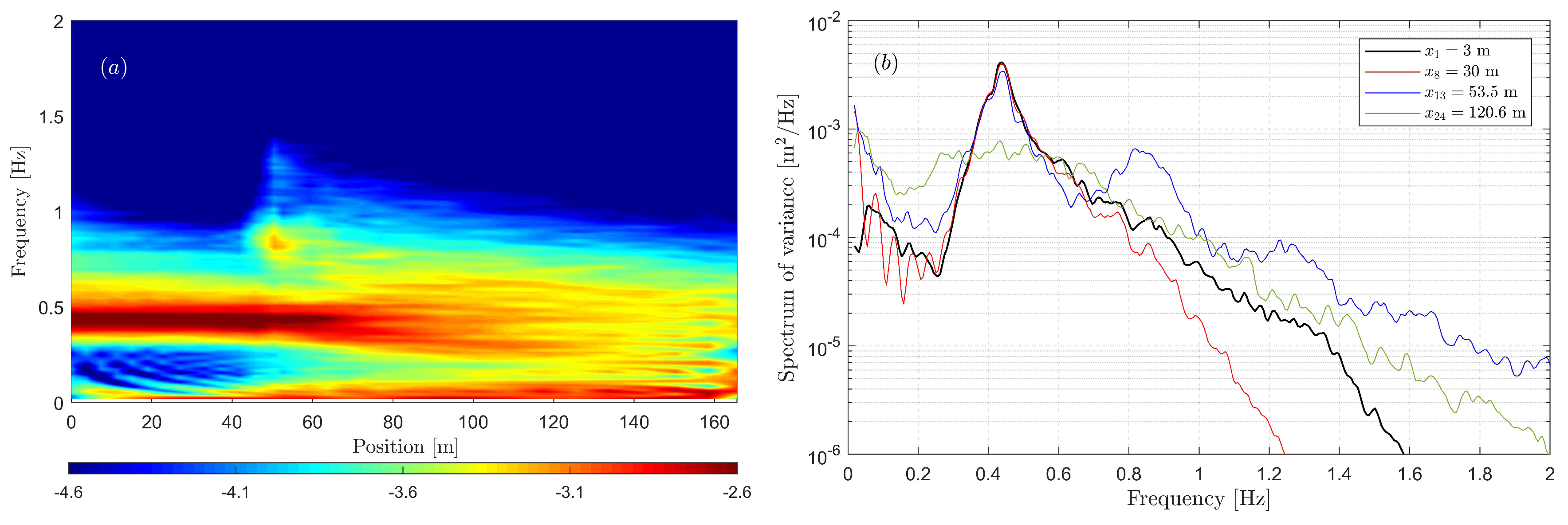
In
Figure 4, both the overall spatial evolution of the spectrum and the detailed spectra at four specific positions are shown. It was observed that, as waves propagate over the deeper region, the wave spectra are modulated mainly in the low-frequency range (
Hz), and several low-frequency modes are formed before the bottom slope. The low-frequency part is a result of the reflection of unabsorbed long waves and the excitation of the natural modes of the wave flume. The wavemaker and the damping zone only “absorb” a part of the reflected wave energy. Thus, these low-frequency modes increase gradually during the test. Over the bottom slope, second-order effect gets increasingly significant especially around the end of the slope (see the yellow peak at about
in
Figure 4a for
m and
Figure 4b for the corresponding spectrum). After the slope segment, the increase of the second harmonic disappears rapidly. More and more wave energy transfers to the low-frequency part, and, as a result, the spectrum broadens. After some distance, due to the energy transfer the low-frequency peak even exceeds the “original” spectral peak and becomes the “new” highest peak of the spectrum (see, for instance,
Figure 4b, Probe 24). Apart from the nonlinear wave–wave interactions, the evolution of the spectrum is also affected by the friction resulting from the boundaries, which play an important role in the dissipation of wave energy. The frictional dissipation works as a low-pass filter, i.e., the dissipation is stronger for the high frequency waves than for the low-frequency waves.
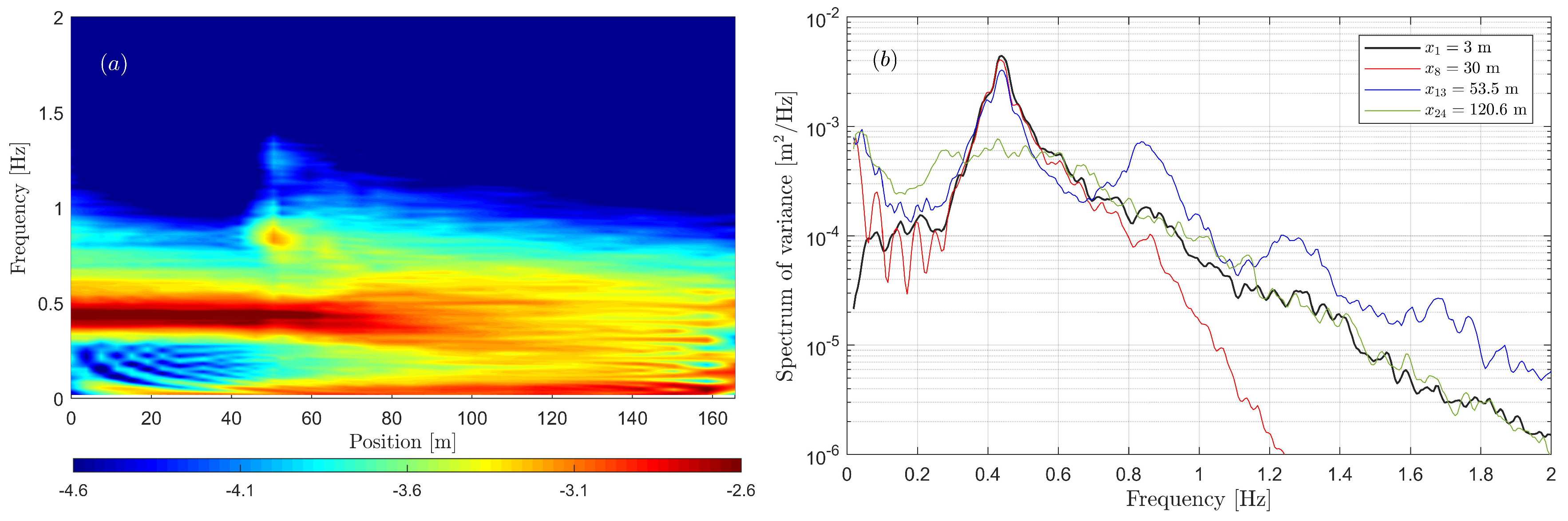
The spectra simulated with the Boussinesq-type model are shown in
Figure 5. The incident wave spectrum shape was well simulated, as waves propagate in the deeper region, the frequencies in the left side of the spectral peak remain in good agreement with the measurements, but differences appear in the higher frequency domain (see
Figure 5b). Potentially, some wave–wave interactions occur between the wavemaker and the first probe generating high frequency components. These high-frequency components are considered as free modes in the simulations due to linear wave making, so that they are dissipated rapidly by friction. Around the end of the slope, the second harmonic clearly appears and is more energetic compared to the measured results. The broadening of the spectrum after the slope is well predicted. In total, the Boussinesq-type model provides a good prediction of spectral evolution, despite the slight overestimation of the nonlinear interaction.
The spectra simulated with whispers3D are shown in
Figure 6. It is shown that the results of whispers3D are in good agreement with the results of the Boussinesq-type model as well as the measurements. Indeed, this model also overestimates the nonlinear wave–wave interactions around the end of the slope so that second (and also higher) harmonic of the spectral peak receive more energy.
5. Data Processing: Bispectral Analysis
It is well-known that waves in nature can be strongly nonlinear when they enter in coastal areas. Especially in the case studied here, the nonlinear effects are significant, and a Fourier analysis is insufficient to interpret the data. A powerful tool to study the nonlinear process is the polyspectral analysis, in particular, the Fourier based bispectral analysis technique which has been used to study the triad wave–wave nonlinear interactions and quadratic phase coupling of nonlinear water waves [
40,
41]. The bispectrum
is defined as the two dimensional Fourier transformation of the third-order auto-correlation function of the signal. Equivalently, it can also be defined as [
42]:
where
is the ensemble average of the triple product of complex Fourier coefficients of two frequencies
and
and their sum
. The asterisk indicates complex conjugate. For time series with zero mean, the Fourier coefficients
come from the following decomposition:
This definition is economic regarding the computational effort thanks to the Fast Fourier transform (FFT) algorithm. The bispectrum has symmetry properties, i.e., , which can further simplify the computation.
In the following, the Fourier coefficients
were computed in the same way as introduced in
Section 4, except that
-point FFT was used to get a smoother bispectrum. In
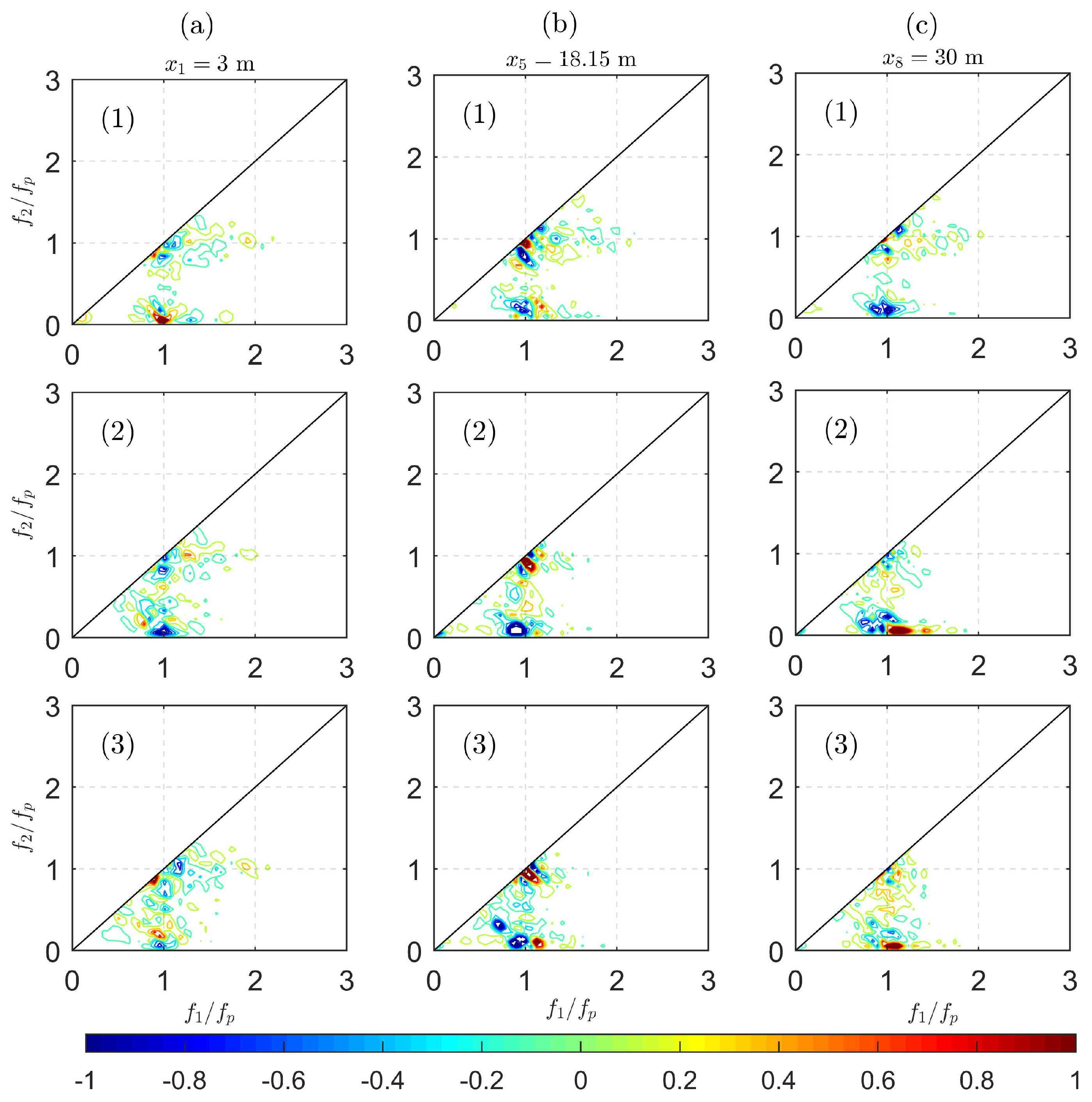
Figure 7,
Figure 8 and
Figure 9, the imaginary parts of the bispectra are plotted, for both the experimental (upper row) and numerical results (second row for the Boussinesq-type model and lower row for the whispers3D model). The two component frequencies
and
were normalised by the incident peak frequency.
The positive and negative values are represented by the colors in the graphs indicating, respectively, the sum interactions and the difference interactions between the two frequency components. For instance, assume , it means that three wave components Hz, 1 Hz and Hz participate in the nonlinear interaction and the wave energy is transferred from Hz to the Hz and 1 Hz components. Similarly, if , the Hz component gain energy from the Hz and 1 Hz components.
Figure 7 shows that, in general, the wave–wave interaction between
and
is weak in the deeper region. In
Figure 7a1, two relatively strong interactions happen around
(red) and
(blue), which indicates that the wave energy is transferred from both the low-frequency modes around
and the second harmonic
to the frequencies around the peak. As waves propagate in the deeper region, in
Figure 7b1, it is shown that for the low-frequency domain both sum and difference interactions are present. This pattern indicates that the energy of peak frequency is transferred to both lower and higher frequencies and that the spectrum broadens. This pattern can hardly be seen in the corresponding spectrum due to weak interactions, but as shown below, the spectral broadening is more obvious in the shallower region. In the simulations, this energy transfer is overestimated, resulting in slightly larger long waves. When waves arrive at the end of the deeper region,
Figure 7c1 shows that the spot around
is blue, meaning that the energy transfers mainly from the peak frequency to the low-frequency components and that long waves are generated. In the deeper region, the simulated and measured bispectra are in overall good agreement.
In
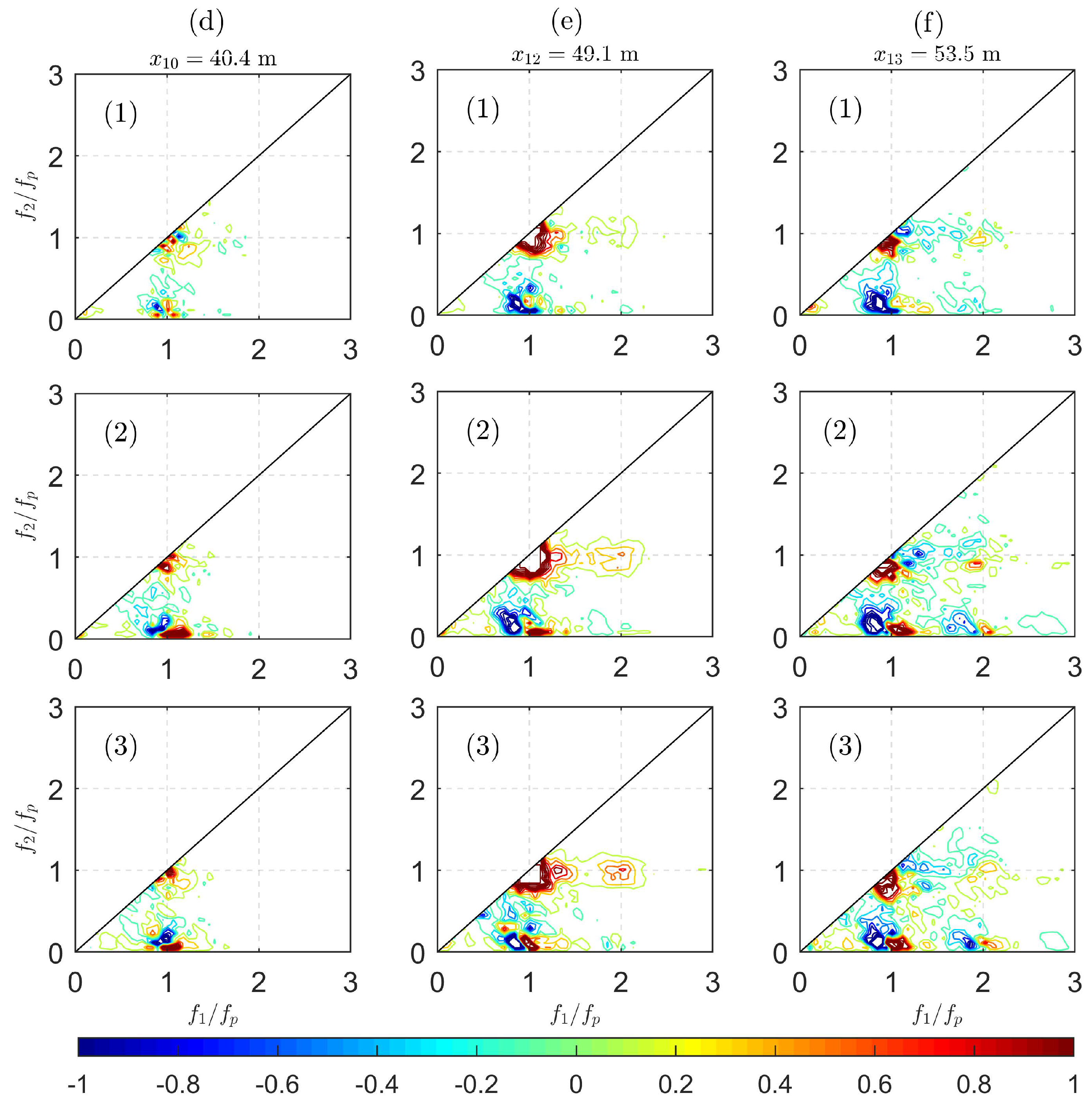
Figure 8, the bispectra of waves propagating over the sloping bottom area are shown where strong nonlinear effects are expected. In
Figure 8d1, it is observed that the nonlinear effect is present but still moderate. In
Figure 8e1, the wave–wave interaction is strong, resulting in an increase of the second harmonic
and the low-frequency waves around
. In
Figure 8f1, not only similar characteristics regarding the second harmonic and the long wave generation are seen, but also the wave–wave interactions between
and
coupled to
is visible. The long waves are generated from both peak frequency and its second harmonic
(see the blue spots at
and
). In the simulations, the agreement is still good but the intensity (or “magnitude”) of nonlinear transfers is slightly overestimated. For instance, the sum interactions of low-frequency modes around
at all three probes are stronger in the two numerical models than in the experiments. As is shown in
Figure 8e2 and e3, the sum interactions at
are also a bit stronger in the simulations.
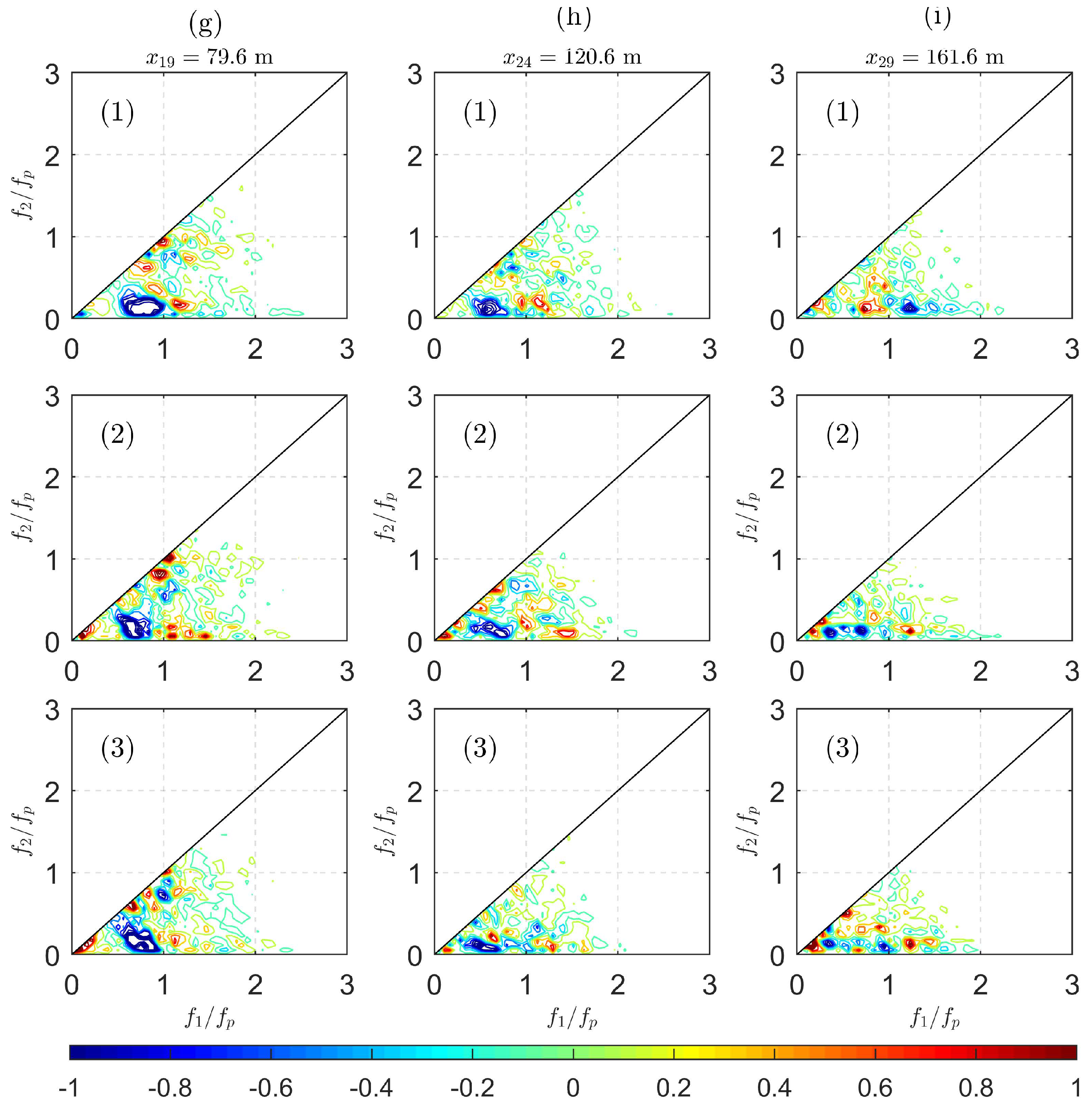
In
Figure 9, three probes are chosen to illustrate the modulation of waves propagating over the shallower region. More wave components participate in the wave–wave interaction, and the contours become more complex. A negative band ranging from
to
is observed which indicates the strong energy transfer from the spectral peak to the bands with frequencies lower than the peak. This blue band is clear in
Figure 9g1, and disappears in
Figure 9i1 because, as the spectral peak keeps losing energy, this energy transfer becomes weaker and weaker. This explains partially the spatial evolution of the spectrum, namely the decrease of the “original” spectral peak, the increase of the low-frequency components (which eventually become new spectral peak) over the shallower region, and the increase of the long wave energy. Another possible reason for this spectral change is the different frictional dissipation rates for different frequencies. The friction dissipates more energy of high-frequency waves while low-frequency wave energy is less dissipated. Finally, a quasi-steady state is reached and the spectral shape keeps almost unchanged, as can be observed for the spectral shape after 100 m in
Figure 4a.
6. Data Processing: Nonlinear Wave Parameters
The free surface elevation is regarded as a stationary stochastic process. In a Gaussian sea state, the characteristic of the statistics of the surface motion can be fully described by its mean
and variance
. As waves propagate into coastal areas, the sea states become non-Gaussian and the nonlinearities affect the wave shape, resulting in sharper and higher wave crests. Higher-order moments can be used to characterise nonlinear effects. Usually, skewness (third-order normalised moment) and kurtosis (fourth-order normalised moment) are considered. They can be computed from time series
:
The skewness is related to the bound mode harmonics and the asymmetry of the probability density function (PDF) of
, and the kurtosis is related to the sharpness of the PDF [
43]. For Gaussian sea states,
and
are expected. For non-Gaussian sea states,
represents asymmetric wave shape (sharper crests and f troughs) and the reverse for
.
indicates an increased probability of occurrence of the largest wave heights [
23], but it is not guaranteed that, when
, the large waves (especially freak waves) will not manifest.
Statistical parameters can also be computed based on the bispectrum. Skewness can be defined as the normalised integral of the real part of the bispectrum [
40]; the wave profile asymmetry w.r.t. the vertical axis is related to the normalised integral of the imaginary part of the bispectrum [
44]:
In
Figure 10, the statistical parameters of the simulations as well as the measured results are shown, and the two different computation methods of the skewness are also compared. It can be seen that the two methods give very similar results; the small differences are probably due to the use of Hann function window (even though a correction factor has already been considered) when computing the Fourier coefficients. It can be seen that both the Boussinesq-type and whispers3D models have good agreement over the two flat bottom regions, but clearly overestimate the maximum skewness (triad wave–wave interaction) around the end of the slope. While the generated waves are almost symmetric w.r.t. the horizontal axis, they become skewed as they propagate over the slope. Around the end of the slope, the wave shape is highly asymmetric w.r.t. the horizontal axis, and the symmetry is not fully recovered in the shallower flat bottom. Regarding the asymmetry parameter, the simulated results agree well with the measured results. As can be seen, this parameter is almost zero except over a short region after the slope which implies that the waves generated are almost symmetric w.r.t. the vertical axis. It is also noted that the presence of the current bottom slope has limited effect on the asymmetry parameter.
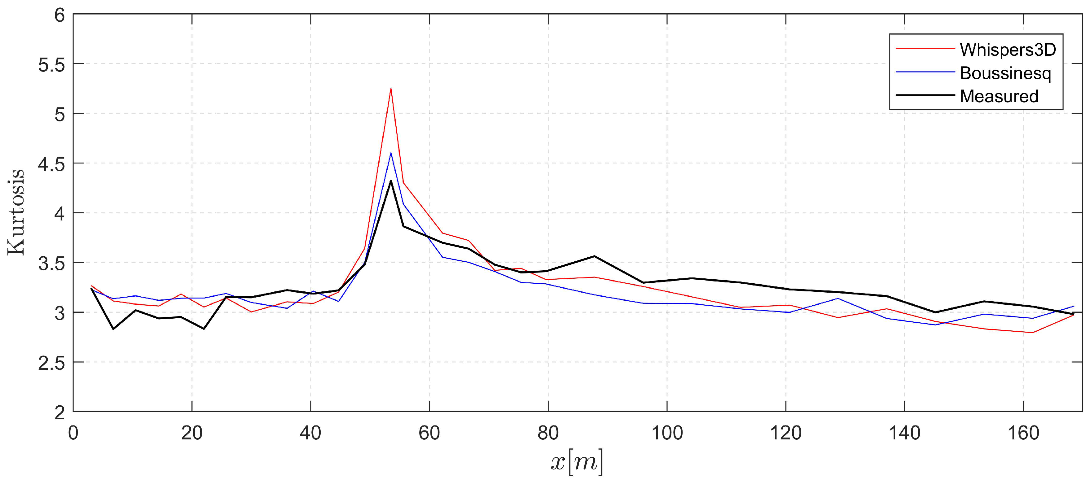
In
Figure 11, the evolution of the kurtosis is shown. It fluctuates around 3 except for the area around the end of the slope, where a local maximum value is observed. This corresponds to the location of Probe 13. The numerical models predict well the overall evolution of kurtosis along the bottom profile. However, they both overestimate the kurtosis around the end of the slope, and this trend is more marked with whispers3D. This is probably because the breaking events in the experiments, which are not considered in the simulations, limited the maximum wave heights. At the end of the slope, the prediction of whispers3D is more non-Gaussian compared to that of the Boussinesq-type model. According to previous studies (e.g., [
23]), the local maximum of kurtosis indicates higher probability of the occurrence of extreme waves. This motivates further investigations of wave height statistics in similar, however, more complicated configurations.
8. Discussion and Conclusions
To achieve a better understanding of the generation mechanism of extreme waves in coastal areas, large scale experiments at THL and highly accurate numerical simulations with two advanced models were performed. A variable bottom profile was designed to study the effects of a constant bottom slope connecting two flat regions on the occurrence of extreme waves. The experimental conditions were chosen based on two non-dimensional parameters: the wave steepness and the relative water depth. Note that our experimental set-up is different from previous experiments [
23,
24] regarding the length of slope, the arrangement of the two flat regions, and, most importantly, the nonlinear effects were relatively strong in the experimental cases shown here. Besides, the large scale facility allowed investigating the whole life cycle of the extreme waves. Spectral, bispectral and statistical analyses of the collected data were conducted, through which a more comprehensive understanding of the shoaling process has been drawn.
In line with previous studies [
23,
25,
26,
27], second- and third-order effects appear in the frequency spectrum, and local maximum values of the statistical parameters skewness and kurtosis were observed in the shallower region. It was experimentally observed that the second-order effects rapidly weaken after the end of the slope, as shown
Figure 4a. The values of skewness and kurtosis also decrease with the weakening of second-order effect: the skewness decreases to a new level instead of zero due to the asymmetrical wave shape in the shallow water, while the kurtosis decreases back to 3.
The imaginary part of the bispectra was used to demonstrate the phase coupling of wave components and the energy transfer due to nonlinear wave–wave interactions. The nonlinear wave coupling is relatively strong around the end of the slope where mainly second and third harmonics are generated. The generation of third harmonic is small in magnitude, but it can be seen in the variance spectrum. Thus, we speculate that the increase of the occurrence probability of extreme waves is more related to the second-order effects. It was also observed in our experiments that a series of low-frequency waves appear. It is anticipated from the bispectra that long waves are mainly generated by the difference interactions as waves propagate in the flume. The frictional dissipation works as a low-pass filter on the wave spectrum, which has limited effects on these low-frequency modes.
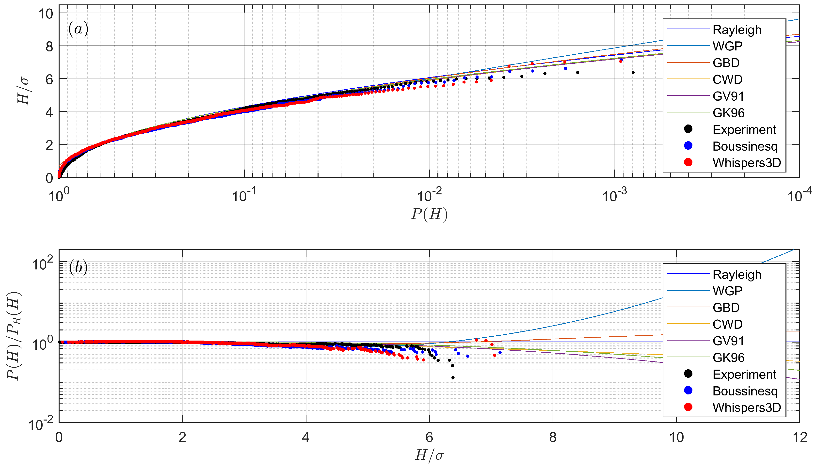
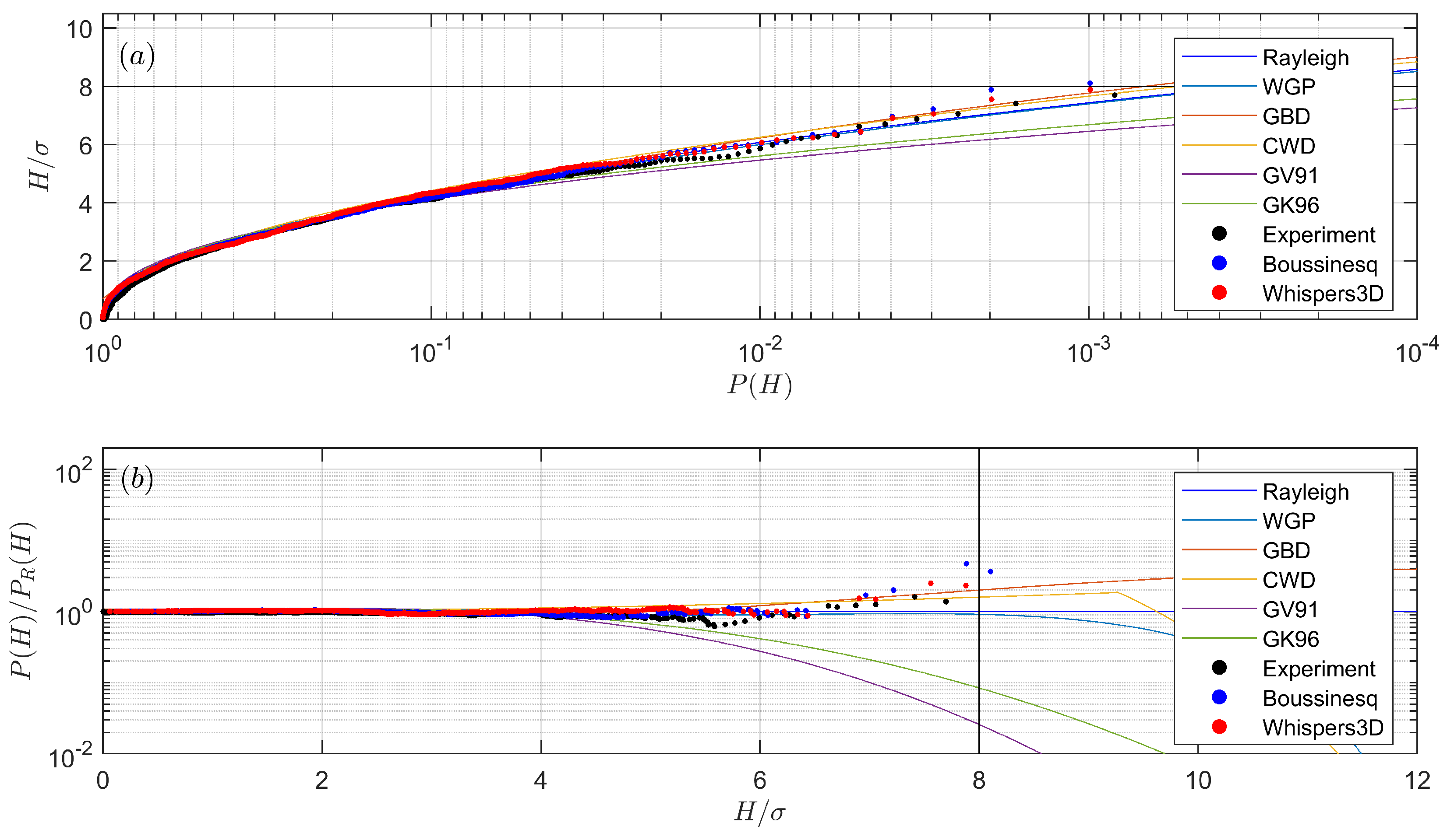
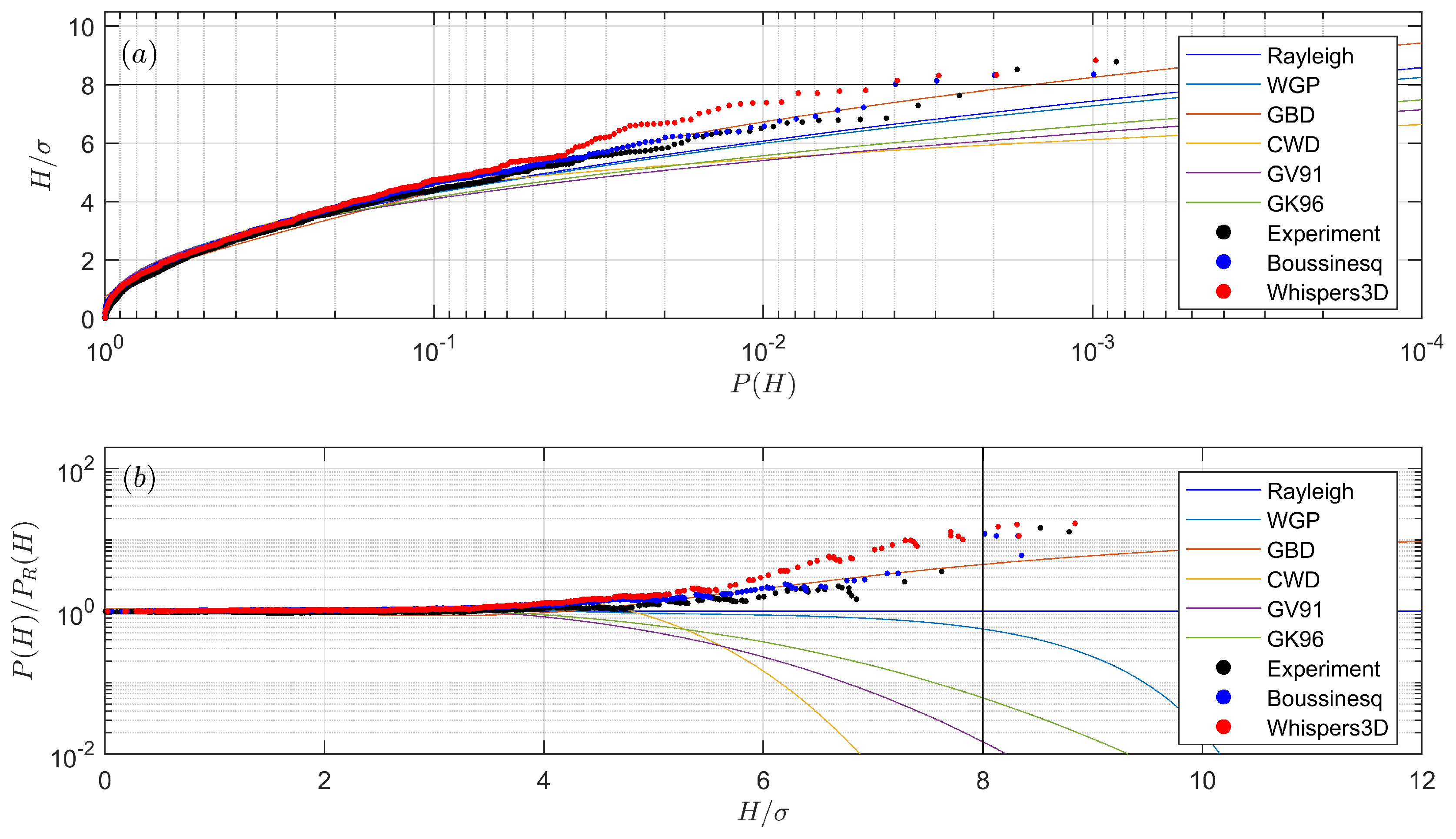
In the deeper region, the sea state is almost Gaussian, and the nonlinear wave–wave interactions are moderate. The wave heights are well described by Rayleigh distribution, except that the latter slightly overpredicts the occurrence probability of the highest waves. The occurrence probability of large waves is significantly increased when waves propagate over the slope. This is due to the fact that the sea state is transforming from one equilibrium state (in the deeper region) to another (in the shallower region). During this process, some of the largest waves can be identified as freak waves and will propagate for a distance while keeping their wave form. We also emphasise that the process of settling down to the new state takes time and a certain distance (a distance-lag in response to the depth transition), thus the shallower region after the slope is also prone to freak waves due to this lag. This was clearly noticeable in our flume set-up, which contains a long flat shallower region. Since the nonlinearities obviously come into play, nonlinear wave parameters are useful in describing the sea state, especially the kurtosis is related to the occurrence probability of large waves. It was confirmed that strong modifications of the distributions of the largest wave are rather well correlated with larger values of the skewness and kurtosis (see
Figure 10 and
Figure 11). The Rayleigh distribution is no longer suitable to describe such sea states, thus a number of wave height distribution models were introduced and compared. In the coastal areas with intermediate or shallow water depth, the wave height distribution models are either semi-empirical or analytical with strong assumptions. In this study, not only the modified Glukhovskiy distributions (GV91 and GK96) and two-part distributions such as CWD and WGP were considered, but also another deep water wave height distribution, GBD, was introduced. This distribution is known to have good predictions for extreme waves [
54]. As the non-equilibrium statistics appear and fade out over the slope, the probability for large waves increases then decreases in the same manner. It was seen that no distribution model can predict the measured wave height distribution equally well for all probes, but, in the prediction of the occurrence probability of large waves, the generalised Boccotti distribution works reasonably well, although it was originally designed for weakly nonlinear deep water waves. The listed shallow water wave height distribution models underestimate the wave height distribution mainly because they assume waves break during the shoaling process.
The numerical results of the Boussinesq-type model and the whispers3D model agree well with the experimental data. The results are in better agreement in the deeper region than in the shallower region, especially before the reflected long waves reach the probes. In particular, the agreement deteriorates due to the contamination of reflected long waves. A small number of wave breaking events also affect the agreement after the slope. These effects are insignificant at the beginning, but the disagreements accumulate as waves propagate in the flume, and eventually affect the simulated results in a significant way. The agreement is acceptable for the deeper region and the slope area, which is of most interest. Two models show very similar results as they both adopt fully nonlinear FSBC and are capable of accounting for variable bathymetry. We noticed that both models overestimate the nonlinear interactions around the end of the slope. The possible reasons for this are numerous; we anticipate that this is due to the non-equilibrium statistics provoked by the transition of water depth. The small number of wave breaking events may also play a role in constraining the maximum achievable skewness and kurtosis. As a further study, new unidirectional irregular wave experiments in the same facility, but with a new bottom profile containing two constant slopes will be conducted and studied in the future. Finally, it is recalled that wave obliquity and wave directionality were not considered in this study; the effects associated with multidirectional (three-dimensional) sea states are left for future work.


