Abstract
The coupled nonlinear Schrödinger equation (CNLSE) is a wave envelope evolution equation applicable to two crossing, narrow-banded wave systems. Modulational instability (MI), a feature of the nonlinear Schrödinger wave equation, is characterized (to first order) by an exponential growth of sideband components and the formation of distinct wave pulses, often containing extreme waves. Linear stability analysis of the CNLSE shows the effect of crossing angle, , on MI, and reveals instabilities between , , and . Herein, the modulational stability of crossing wavetrains seeded with symmetrical sidebands is determined experimentally from tests in a circular wave basin. Experiments were carried out at 12 crossing angles between , and strong unidirectional sideband growth was observed. This growth reduced significantly at angles beyond , reaching complete stability at = 30–40. We find satisfactory agreement between numerical predictions (using a time-marching CNLSE solver) and experimental measurements for all crossing angles.
1. Introduction
Crossing seas, in which waves travel in multiple directions, have been identified as an important challenge to offshore operations, linked to an increased probability of extreme waves [1,2]. In addition to specific environmental forcing such as wind or (sudden) changes in bathymetry, two important mechanisms play a role in the formation of so-called rogue waves in the ocean, namely random dispersive focusing enhanced by weak bound-wave nonlinearity and modulational instability [3,4,5,6]. Herein, we contribute to the understanding of extreme waves in crossing seas by reporting on an experimental study of modulational instability in waves crossing at angles between .
For long-crested or unidirectional seas, it is well established that weakly nonlinear regular wavetrains in sufficiently deep water rapidly evolve into pulses of wave groups through modulational instability (MI) [7,8]. Extreme waves can form within such groups, making MI a topic of considerable interest in the context of rogue wave events. The nonlinear Schrödinger equation (NLSE) provides the simplest mathematical framework for studying MI, and permits unstable solutions including breathers and plane Stokes waves [9,10]. Breather waves are characterized by a sudden increase in amplitude of initially regular waves to either three or five times their initial value [11,12], and provide close approximations to rogue waves in long-crested seas. However, experimentally, breather waves are particularly sensitive to initial conditions, which must be specified precisely for the waves to attain maximum amplitude [13]. Particularly, in the case of the Peregrine breather, which is localized in both time and space, precise initial conditions lead to an extreme wave only once during its evolution. Although precise reproduction of specific breather solutions in the laboratory requires special input conditions at the wavemaker, such initial conditions do not exist in the ocean. Nevertheless, clear evidence of breather trains has been observed in measured ocean wave data sets through the nonlinear Fourier method [14]. Moreover, in the laboratory, breather trains have been observed to be stable to disturbances such as from wind [15].
The unstable regular Stokes wave seeded with sideband components to the carrier has periodic modulations that grow, facilitating straightforward measurement of wavetrain stability, such as in the seminal paper by Lake et al. [16]. In this idealized problem, energy is returned from the sidebands to the carrier wave at later times, leading to periodic modulation and demodulation on very long time scales known as Fermi–Pasta–Ulam (FPU) recurrence [17,18,19]. Strictly, FPU recurrence only exists in conservative systems and is prevented by the occurrence of breaking. In the case of breaking, the principle of time-reversibility also does not apply [20]. However, even in the presence of breaking waves, energy from sidebands returns to a central carrier wave after some time, giving rise to FPU-type modulation-demodulation cycles [16,21]. This paper avoids these complications in all experiments by considering only the initial stages of modulational instability, before breaking takes place.
Although extensively studied both theoretically and experimentally in one dimension, the applicability of the 1D+1 NLSE to the open ocean is limited by the equation’s unidirectionality. In the open ocean, waves may be created from multiple sources, interact, and cross at an angle. Additionally, in fetch-limited seas it has been observed that spectral components above and below the peak frequency become bimodal with energy naturally spreading symmetrically to angles above and below that of the peak frequency direction [22,23]. As derived for deep-water by Onorato et al. [24] from the 2D+1 Zakharov equation [25], the coupled nonlinear Schrödinger equation (CNLSE) is a system of nonlinear wave equations describing the interaction of two narrow-banded weakly nonlinear wave systems propagating at an angle (see also [26]). This deep-water CNLSE has since been extended to finite depth by Kundu et al. [27]. However, for practical purposes, the experiments presented herein were performed in deep water. The CNLSE enables both MI and crossing effects to be explored simultaneously. By invoking the assumptions of symmetrical propagation about the x-axis at angle and shared group velocity along the x-axis, the CNLSE simplifies and readily lends itself to linear stability analysis. The results define both low angle and high angle instability regions separated at and (see also [28]). Discussions concerning linear stability of CNLSE and the effect of the changing values of CNLSE coefficients with crossing angle have highlighted increased amplification factors but decreased growth rates of breather and soliton solutions in crossing seas for angles approaching [29,30]. Within this paper, crossing angle, is the angle at which waves propagate to the x-axis, i.e., when two waves cross at the angle of bisection is . Along with the general investigation into plane wave stability, rogue wave solutions to the CNLSE are known to exist and have been classified and, through numerical computations, compared to their 1D+1 analogue, the Peregrine breather [31].
Laboratory experiments by Toffoli et al. [32] have measured the long-term statistical behaviour of deep-water weakly nonlinear crossing waves up to crossing angles of (see Figure 1b for these experimental angles). Numerical solutions using a higher-order spectral method were used to confirm these findings and additionally, to study crossing angles up to and found increases in kurtosis for crossing angles in the range [33]. Additionally, the effect of oblique sideband perturbations (of up to ) to plane waves propagating over finite depth were investigated experimentally and sideband growth was reported [33]. The existence of short-crested crossing breather waves (slanted breather solutions to the 2D+1 NLSE) has also been confirmed experimentally [34].
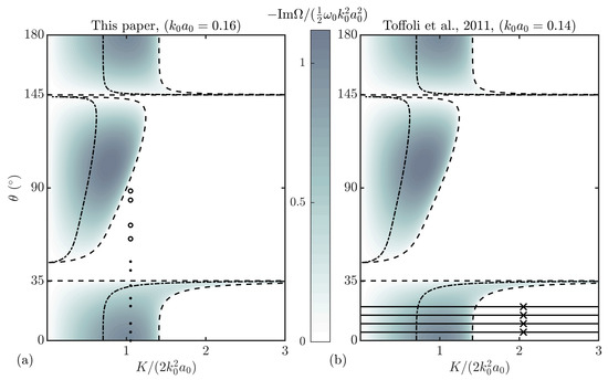
Figure 1.
Surfaces showing the growth rate obtained from linear stability analysis of the coupled nonlinear Schrödinger equation (from (11)). Panel (a) presents our experimental parameters where experiments 2a-h are indicated by dots (results presented in main text) and experiments 2i-l by open circles (results presented in Appendix B). The crossing angles of experiments performed by Toffoli et al. [32] are shown as solid lines in panel (b) with the crosses and y-axis marking the boundary containing of the spectral energy (note that the crossing angle, , in Toffoli et al. [32] is equivalent to ). The dashed lines indicate boundaries of stability regions, while the dot-dashed lines show the boundary between complex () and simple () evolution.
In addition to possible MI, changes to the second-order bound waves occur when waves cross. The wave-averaged free surface, represented spectrally by second-order difference waves, is the local mean surface elevation formed by temporal averaging over the rapidly varying waves that make up the slowly varying group. Whereas a set-down of the wave-averaged free surface is expected in the absence of crossing, packets are accompanied by a set-up for sufficiently large crossing angles. This can be theoretically predicted [35,36,37,38] based on second-order interaction kernels [39,40,41,42]. Set-up has been observed in field data [43,44,45] and recently in detailed laboratory experiments [46]. For the Draupner wave, recorded in the North Sea on the 1st of January 1995 [47], the observation of set-up can be seen as evidence for crossing [43,48,49]. In fact, linear dispersive focusing enhanced by bound-wave nonlinearity but without MI may be sufficient to explain observations such as the Draupner wave [50,51].
Recently, a number of additional numerical studies have examined extreme waves and MI in crossing seas. Støle-Hentschel et al. [52] have shown, using numerical simulations and laboratory experiments, that a small amount of energy travelling in exactly the opposing direction can significantly reduce the kurtosis of the surface elevation. Gramstad et al. [53], using random simulations of the Zakharov equation, found that, for unimodal spectra, kurtosis increased at crossing angles close to and at very small crossing angles when compared to the unidirectional case. Kurtosis was found to be at a minimum at .
In this paper, we report on regular wave experiments with seeded sidebands for two crossing wavetrains in a circular wave basin. These experiments are the crossing-wave counterpart of the classical experiments by Lake et al. [16] and cover both stable and unstable regions of the space, through the range , where K is the perturbation wavenumber. We measure the growth of sidebands and compare this to results from linear stability analysis of the CNLSE, as well as numerical solutions of this equation.
2. Theoretical Background
2.1. Coupled Nonlinear Schrödinger Equation (CNLSE)
The coupled nonlinear Schrödinger equation (CNLSE), derived by [24] from the 2D+1 Zakharov equation [25], is a narrow-banded wave equation describing the evolution of coupled, complex wave envelopes A and B. Both wave envelopes propagate on an associated carrier wave whose properties define the CNLSE coefficients and thus (along with the initial conditions) the envelope evolution. Scaled for water waves, and under the assumption of identical but symmetrical carrier waves (about the x-axis) with distinct amplitude envelopes, the CNLSE is given, in a Cartesian coordinate system , by [24],
where carrier properties: frequency, ; x-axis wavenumber, k; y-axis wavenumber, l; and absolute wavenumber, , define the group velocities and along their respective axes,
the linear coefficients , , and are given by,
and the nonlinear coefficients and by,
The carrier frequency and absolute wavenumber are related through the deep-water dispersion relation, , with g denoting the gravitational constant.
In the special case of envelopes propagating along the x-axis, a Galilean transformation into the group reference frame reduces the CNLSE to [24],
where . From the wave packet amplitudes, the (linear) free surface elevation is reconstructed by reintroducing the carrier waves through,
2.2. Linear Stability Analysis
Linear stability analysis of the CNLSE reveals many properties of the equation and, using a seeded carrier solution, allows prediction of the initial sideband growth rate. Identical plane waves are admitted as solutions to (6) and (7) and we therefore add perturbations of infinitesimal amplitude and phase to obtain (see also [24]),
where and are carrier amplitudes, and , , , and are small perturbations in amplitude and phase. In this linear stability analysis, the assumed form of the sideband solutions and is,
where and are the initial sideband amplitudes, K is the perturbation wavenumber, and is the perturbation frequency. The relationship between K and is found through linear stability analysis as [24],
where it is apparent that may take either real or imaginary values. Following substitution of this relationship into (10), either oscillatory (when Re) or exponential (when Im) behaviour can be expected from the sidebands.
Figure 1 presents the instability regions in -space with stability boundaries denoted by the critical perturbation wavenumber function, . Three regions of instability exist: at low angle, ; medium angle, ; and high angle, , in which is related to the carrier wavenumbers through . We note that the asymmetry around (i.e., comparing the region from towards an increasing angle and the region from towards decreasing ) arises because the perturbation always travels in the positive x-direction. Figure 1a also shows where in space the experiments reported on herein lie, with Figure 1b displaying the locations of experiments previously reported by Toffoli et al. [32]. These experiments are restricted to angles and are carried out with a continuous spectrum instead of discrete sidebands, as illustrated by the horizontal lines in Figure 1b, with of their energy bounded by the y-axis and the black crosses.
For unidirectional waves, MI behaves as described by the standard NLSE but with increased instability due to the presence of two carrier waves, with a consequent doubling of steepness. As the crossing angle is progressively increased, the region of instability extends further along the wavenumber axis, whereas the magnitude of the instability decreases gradually. At (exactly, ), the low angle instability region ends, having encompassed all wavenumbers. At approximately , the medium-angle instability region begins to take shape, starting close to zero wavenumber and expanding along the wavenumber axis until the crossing angle reaches approximately . Finally, the high-angle region commences as a sharp boundary at approximately and ends as a mirrored version, similar to the low-angle region (with both waves travelling at from the x-axis).
2.3. Characteristics of Modulational Instability: Complex vs. Simple Evolution
Figure 2 presents the spectral and temporal evolution of two modulated wavetrains with different perturbation wavenumbers propagating from the initial conditions (9) with and , obtained using a numerical solver of the CNLSEs (see Appendix A). The effect of MI is instantly recognizable from the increase in amplitude of the sidebands closest to the carrier wave (primary sidebands). As the primary sideband amplitudes increase, the carrier amplitude begins to decrease. Further in the evolution process, secondary sidebands appear at integer multiples of the primary sideband wavenumber. The effect of this initial stage of instability is seen in the packet amplitude in Figure 2b as a rapid increase in the group amplitude. Following the exponential sideband amplitude growth, Fermi–Pasta–Ulam recurrence is observed. During idealized FPU recurrence, energy is exchanged periodically between modes, and the system returns to its original state [17,18,19]. However, in water waves, energy may be lost to wave breaking resulting in a nonconservative system but we note that FPU recurrence is a long-term behaviour, and strong MI is required to observe it in the space available in most experimental facilities.
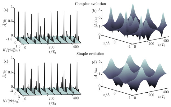
Figure 2.
Spectral and temporal evolution obtained from the time-marching of the CNLSE for two unstable modulated wavetrains crossing at . Panels (a,b) show complex () evolution, whilst panels (c,d) display simple () evolution. Temporal axes have been normalized by the carrier wave period, .
Figure 2a,b show the wavetrain propagating with complex recurrence, whereas Figure 2c,d show simple recurrence. Complex recurrence is expected when K lies less than (or at) half-way through the instability region (), and primary sidebands themselves act as unstable carriers, continually spawning new sidebands. When K lies more than half way to the stability boundary () new sidebands will lie in the stable region, and simple recurrence is observed.
3. Experimental Methodology
3.1. Facility
The aim of our experiments was to measure sideband growth at extreme crossing angles up to . In order to achieve this, physical tests were performed in the FloWave Ocean Energy Research Facility at the University of Edinburgh, which is capable of omnidirectional wave creation and absorption. The basin (depicted in Figure 3a,b) has a diameter of , a working depth of , and is encircled by 168 actively absorbing force-feedback wavemakers. A Cartesian coordinate system was defined with its origin at the centre of the basin. The primary direction of propagation of the waves was in the positive x direction. In crossing wave experiments, the carrier waves travelled at an angle, , from the x-axis, as defined in Figure 3a. Wave generation in the facility was controlled using software based on linear wave theory. Ten resistance type wave gauges at a spacing of were mounted on a gantry spanning the basin x-axis (see Figure 3b for coordinates). Wave gauges were calibrated each day before tests commenced. A 20 min settling period was imposed between each test, allowing residual basin motion to settle to an acceptable level.
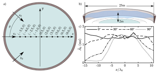
Figure 3.
(a) FloWave Ocean Energy Research Facility at The University of Edinburgh, showing wave gauge locations relative to the centre of the basin (units in ) and direction of wave system components (figure adapted from [54]). (b) Sectional view of the FloWave basin with key dimensions. (c) Amplitude profiles of unseeded carrier waves () travelling at an angle, , and measured along the basin x-axis (Part I).
3.2. Matrix of Experiments
The experimental campaign was split into two parts. Part I aimed to quantify the effect of finite-length crests in the facility in the absence of seeded sidebands, which is a manifestation of the inability of a finite number of wavemakers encircling a finite-size circular basin to create perfectly long-crested waves spanning the entire basin diameter. This finite-crest effect needed to be quantified in order to estimate the length over which components travelling with different directions would interact. Part II aimed to measure the growth of frequency sidebands about carrier waves travelling at crossing angles . Crossing carrier and sideband waves only interact fully in regions of total crest overlap, and so the extent that these regions cover the chosen wave gauge locations is defined by the carrier crest length and angle. Experiments 1a–d (Part I) were therefore designed to determine the effective sideband evolution region in the basin at each angle. In these experiments, a single unseeded carrier wave was propagated at the angles given in Table 1 (Part I).

Table 1.
Experiment labels and their corresponding crossing angles for both Part I (single, unseeded regular wave) and Part II (seeded waves). All experiments used carrier parameters of , , and . Experiments 2a–l used sideband parameters of , and .
For Part I, the amplitude profiles of experiments 1a–d are presented in Figure 3c and allow estimation of the carrier crest length in the FloWave facility. Experiment 1d () shows that, for high angle experiments, a reasonable region in which to expect full sideband-carrier interactions occupies approximately 10 wavelengths centred about the basin origin. However, the effective length is extended significantly to more than 20 wavelengths for crossing angles up to , the region of greatest interest in Part II. As expected, for waves in the x-direction (), the region covers all wave gauge locations. The results from the Part I tests were interpolated in order to estimate the finite-crest effect at all crossing angles.
All experiments in Part II were performed with constant values of carrier frequency, , carrier amplitudes , and initial sideband amplitude , giving a depth parameter , and steepness of a single carrier, . Figure 1a shows the expected growth rates, crossing angles, and sideband wavenumbers for the Part II tests. A simple system of four plane waves, consisting of two carrier waves propagating at to the x-axis, and two sidebands propagating along the x-axis was used as input to the wave generation software. Explicitly, we thus have,
where is the x-position of the wavemaker along (the axis of propagation of the sidebands). The relatively high carrier frequency was chosen to slow group velocity, increasing the effective evolution distance. The carrier amplitude was subsequently calculated to give a moderate steepness of , required for prominent instability but to avoid breaking. Each experiment was repeated 3 times.
3.3. Data Processing
The calibrated wave gauge outputs (free surface time histories) from each experiment were band-pass filtered to eliminate higher-order and low-frequency bound waves. The recorded free surface elevation time series length was limited to eliminate reflected waves. A Tukey window with a tapering parameter of was used to create a transient signal and limit the lobe effect associated with windowing. The length of the Tukey window was determined using the estimated linear group velocity of the wavetrain. The amplitude spectrum was determined at each location (see Figure 4), and the evolution of the primary sidebands (frequency components located closest to the carrier wave) used to identify MI. The true frequency of these components was determined at the first gauge location. These component amplitudes were then tracked across all the remaining wave gauges. Sideband and carrier amplitudes at the first wave gauge location were used as initial conditions for a CNLSE solver (using the Fourier, split-step method, see Appendix A) and as inputs to the prediction by the linear stability analysis (11). The experimental evolution of the sidebands is compared to these numerical solutions, as well as the linear stability analysis (11) below.
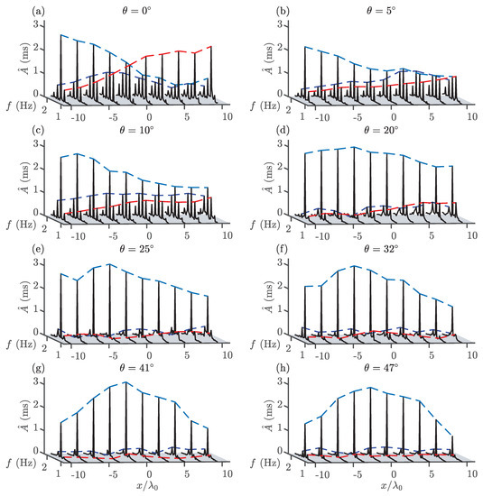
Figure 4.
Amplitude spectra for experiments 2 (a–h) (Part II) obtained using the measured free surface time series along the primary wave propagation direction (see Figure 3a for gauge locations) for different crossing angles, . Dashed lines follow the amplitudes of the carrier (light blue), lower sideband (red), and upper sideband (dark blue).
4. Results
Figure 4 shows the evolution of the amplitude spectra along the tank’s x-axis (the direction of propagation of the perturbation) for the different crossing angles considered in experiments in Part II. This figure shows both the finite-crest effect we studied in Part I and the effect of modulational instability. Figure 5 presents the evolution of the primary sideband amplitudes of experiments 2a–l. In order to separate out the finite-crest effect and modulational instability, we also show, as light grey thick lines, the amplitude of unseeded regular waves (from Part I). In doing so we identify the region over which the finite-crest effect does not play a role (i.e., the region over which the light grey thick lines are horizontal) and we can exclusively examine modulational instability.
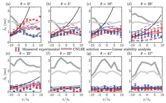
Figure 5.
Comparison of the evolution of sideband amplitude along the centreline of the basin for experiments 2 (a–h) (Part II) from measurements, numerical solutions (crosses) of the CNLSE (thin blue and red lines) and linear stability analysis (thin black lines). Lower and upper sidebands are indicated in red and blue, respectively. Error bars and dashed lines represent one standard deviation from the mean across repeats for the measured data and the CNLSE solution, respectively. Thick lines represent the mean seeded (dark grey) and unseeded (light grey) carrier waves across repeats.
Also shown in Figure 5 are the numerical results from the CNLSE time-marching scheme and the linear stability analysis. For brevity, only experiments 2a–h are presented (see Appendix B for experiments 2i–l, which show stability, as predicted). Each experimental repeat was solved across the spatial domain using the CNLSE solver. The results of the solver were then averaged and the standard deviation across repeats was calculated. Error bars for experimental measurements and dashed lines for the numerical scheme are used to indicate one standard deviation from the mean across repeats. The carrier amplitude evolution is denoted by dark grey lines and the interpolated measurements from Part I are denoted by light grey lines, indicating the region over which an unseeded carrier wave can be considered of constant amplitude.
4.1. Unidirectional Waves:
The unidirectional experiment 2a, presented in Figure 5a, shows the most significant growth in sideband amplitude, with the lower sideband increasing by more than a factor of three. An increase in amplitude can also be observed in the upper sideband and the beginnings of FPU recurrence appear. The numerical solution in Figure 5a also shows significant growth and follows the average of the upper and lower sideband amplitudes well, displaying many of the same characteristics (such as FPU recurrence). However, the lower sideband grows much more quickly than the upper sideband, which is subject to initial growth followed by considerable attenuation, a feature not predicted by the NLSE but predicted in the modified NLSE [55] and commonly observed in unidirectional experiments [21].
The effect of sideband growth and MI on free surface elevation is shown by the formation of pulses in Figure 6. Extreme waves occur in these pulses when carrier crests come in phase with the group centre, as demonstrated in Figure 6a at , where a cluster of three waves has more than doubled in amplitude within . Figure 4a presents the amplitude spectra for experiment 2a. Substantial growth in secondary sidebands is evident. These secondary sideband frequency components, located at multiples of the perturbation frequency, contribute to the growth of wave group amplitudes and further enhance the strong decline of the carrier amplitude.
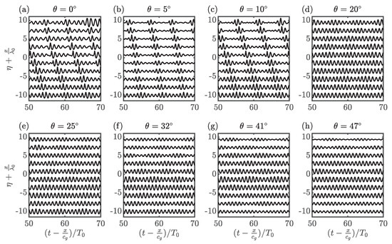
Figure 6.
Measured free surface elevation time series for experiments 2 (a–h) (Part II) shifted by the linear group velocity and normalized by the carrier period, , with the positive vertical axis also representing increasing distance along the basin.
4.2. Crossing Waves:
Figure 5b–d show that the growth observed in the unidirectional case continues but slows as the crossing angle is increased to . In these experiments, the maximum amplification factor of the lower sideband generally reduces compared to the unidirectional case, whereas the upper sideband appears relatively unaffected, with no strong growth in either case. The pulse formations seen in experiment 2a persist in Figure 6b–d along with the sideband growth in Figure 4b–d, though with reduced magnitude. The unseeded carrier wave amplitude profiles of Figure 5b–d (measured in Part I) remain largely unchanged along the length of the basin, indicating that the effective length, over which crests reach their full amplitudes, is sufficiently long. Between and (Figure 5e–g), the transition to stability takes places. Throughout the transition to stability, the amplitude of unseeded regular waves show some drop in amplitude at their fringes. These drops in amplitude indicate the edges of the interaction region caused by the finite-crest effect of the tank. However, up to , 15 wavelengths of interaction distance remain, a distance seen in the unidirectional case to be sufficient for sideband growth to occur. Experiments at angles of and higher (Figure 5g,h, and Appendix B for the measurements from experiments 2i–l) are stable.
5. Conclusions
We have experimentally investigated the effects of crossing angle on the modulational stability of two crossing nonlinear surface gravity wavetrains seeded with sideband perturbations and compared the measurements to predictions by the the coupled nonlinear Schrödinger equation (CNLSE). The results demonstrate that sideband growth, as predicted by linear stability analysis of the CNLSE, can be reproduced in physical experiments undertaken in a circular wave basin. Strong modulation occurred in the unidirectional case, where the beginnings of recurrence were observed. The growth rate reduced as the crossing angle was increased; negligible growth was measured at and beyond a crossing angle of approximately . Due to the reduced growth rate and the finite length of the basin, we have not been able to observe the increased amplification factors associated with angles approaching the medium and high angle instability regions. An unseeded, regular wave was used to estimate the finite-crest effect (an experimental limitation for a finite-size circular basin), which started to become significant at , well beyond the theoretical stability boundary of . Taking into account the reduction in evolution length imposed by the finite-crest effect, no growth in sidebands was found to occur at these high angles. Future work should seek to extend experimental measurements into the second (high-angle) unstable region. To complete this successfully, the finite-crest effect must be considered allowing sidebands enough interaction evolution distance to grow. We envisage this will be challenging in the FloWave basin.
Author Contributions
Formal analysis, J.N.S.; Investigation, J.N.S.; Methodology, J.N.S. and M.L.M.; Supervision, A.G.L.B. and T.S.v.d.B.; Writing—original draft, J.N.S.; Writing—review and editing, M.L.M., A.G.L.B. and T.S.v.d.B.
Funding
FloWave was funded by the UK EPSRC (EP/I02932X/1). J.N.S. acknowledges an EPSRC studentship (No. 1770088), and TSvdB a Royal Academy of Engineering Research Fellowship.
Acknowledgments
The authors would like to thank: Edward Nixon, Samuel Draycott, and Thomas Davey at FloWave for their help designing and carrying out the experiments.
Conflicts of Interest
The authors declare no conflict of interest.
Appendix A. Split-Step Time Marching Technique
The split-step method (also known as the Fourier method) takes advantage of the fact that the linear and nonlinear components can be separated and then solved exactly [56]. The linear component is solved in Fourier space, whereas the nonlinear is solved in the time or space domain (depending on the form of the equation). In the split-step method, the linear and nonlinear components of the CNLSEs are treated independently and the predictions combined immediately after each time step as the full solution advances forward. A known error of (where , the carrier wave steepness) is associated with the independence assumption. The split-step method is second-order accurate in and to all orders in , it is unconditionally stable [57].
First, the CNLSE is rearranged and split into its linear and nonlinear components (here only (6) is considered for brevity),
The nonlinear component is integrated forwards in the time domain as follows,
whereas the linear component is Fourier-transformed,
and then integrated in time to give,
Combining the linear and nonlinear components, at each time step we have the explicit expression,
The same process is applied to (7). The results of advancing A and B individually are combined in the current time step to give the full system state to be passed to the next step.
Appendix B. Experiments 2i–l: 60° ≤ θ ≤ 88°

Figure A1.
Measured free surface elevation time series for experiments 2i–l (Part II) shifted by the linear group velocity and normalized by the carrier period, , with the positive vertical representing increasing distance along the basin.
Figure A1.
Measured free surface elevation time series for experiments 2i–l (Part II) shifted by the linear group velocity and normalized by the carrier period, , with the positive vertical representing increasing distance along the basin.


Figure A2.
Amplitude spectra for experiments 2i–l (Part II) obtained using the measured free surface time series along the primary wave propagation direction (see Figure 3a for gauge locations) for different crossing angles, . Dashed lines follow the amplitudes of the carrier (light blue), lower sideband (red), and upper sideband (dark blue).


Figure A3.
Comparison of the evolution of sideband amplitude along the centreline of the basin for experiments 2i–l (Part II) from measurements, numerical solutions (crosses) of the CNLSE (thin blue and red lines) and linear stability analysis (thin black lines). Lower and upper sidebands are indicated in red and blue, respectively. Error bars and dashed lines represent one standard deviation from the mean across repeats for the measured data and the CNLSE solution, respectively. Thick lines represent carrier wave amplitudes from the seeded (Part II, dark grey) and unseeded (Part I, light grey) experiments.

References
- Bitner-Gregersen, E.; Gramstad, O. Rogue waves impact on ships and offshore structures. In Det Norske Veritas Germanischer Lloyd Strategic Research and Innovation Position Paper; DNV GL: Oslo, Norway, 2015. [Google Scholar]
- Cavaleri, L.; Bertotti, L.; Torrisi, L.; Bitner-Gregersen, E.; Serio, M.; Onorato, M. Rogue waves in crossing seas: The Louis Majesty accident. J. Geophys. Res. Oceans 2012, 117. [Google Scholar] [CrossRef]
- Kharif, C.; Pelinovsky, E. Physical mechanisms of the rogue wave phenomenon. Eur. J. Mech. B Fluid 2003, 22, 603–634. [Google Scholar] [CrossRef]
- Dysthe, K.; Krogstad, H.E.; Müller, P. Oceanic rogue waves. Annu. Rev. Fluid Mech. 2008, 40, 287–310. [Google Scholar] [CrossRef]
- Onorato, M.; Residori, S.; Bortolozzo, U.; Montina, A.; Arecchi, F. Rogue waves and their generating mechanisms in different physical contexts. Phys. Rep. 2013, 528, 47–89. [Google Scholar] [CrossRef]
- Adcock, T.A.; Taylor, P.H. The physics of anomalous (‘rogue’) ocean waves. Rep. Prog. Phys. 2014, 77, 105901. [Google Scholar] [CrossRef]
- Yuen, H.C.; Lake, B.M. Nonlinear dynamics of deep-water gravity waves. In Advances in Applied Mechanics; Elsevier: Amsterdam, The Netherlands, 1982; Volume 22, pp. 67–229. [Google Scholar]
- Benjamin, T.B.; Feir, J. The disintegration of wave trains on deep water Part 1. Theory. J. Fluid Mech. 1967, 27, 417–430. [Google Scholar] [CrossRef]
- Ma, Y.C. The perturbed plane-wave solutions of the cubic Schrödinger equation. Stud. Appl. Math. 1979, 60, 43–58. [Google Scholar] [CrossRef]
- Peregrine, D.H. Water waves, nonlinear Schrödinger equations and their solutions. ANZIAM J. 1983, 25, 16–43. [Google Scholar] [CrossRef]
- Akhmediev, N.; Ankiewicz, A.; Taki, M. Waves that appear from nowhere and disappear without a trace. Phys. Lett. A 2009, 373, 675–678. [Google Scholar] [CrossRef]
- Chabchoub, A.; Hoffmann, N.; Onorato, M.; Akhmediev, N. Super rogue waves: Observation of a higher-order breather in water waves. Phys. Rev. X 2012, 2, 011015. [Google Scholar] [CrossRef]
- Chabchoub, A.; Hoffmann, N.; Akhmediev, N. Rogue wave observation in a water wave tank. Phys. Rev. Lett. 2011, 106, 204502. [Google Scholar] [CrossRef] [PubMed]
- Osborne, A.R.; Resio, D.T.; Costa, A.; de León, S.P.; Chirivì, E. Highly nonlinear wind waves in Currituck Sound: Dense breather turbulence in random ocean waves. Ocean Dyn. 2019, 69, 187–219. [Google Scholar] [CrossRef]
- Chabchoub, A.; Hoffmann, N.; Branger, H.; Kharif, C.; Akhmediev, N. Experiments on wind-perturbed rogue wave hydrodynamics using the Peregrine breather model. Phys. Fluids 2013, 25, 101704. [Google Scholar] [CrossRef]
- Lake, B.M.; Yuen, H.C.; Rungaldier, H.; Ferguson, W.E. Nonlinear deep-water waves: Theory and experiment. Part 2. Evolution of a continuous wave train. J. Fluid Mech. 1977, 83, 49–74. [Google Scholar] [CrossRef]
- Fermi, E.; Pasta, P.; Ulam, S.; Tsingou, M. Studies of the Nonlinear Problems; Technical Report; Los Alamos Scientific Lab.: Los Alamos, NM, USA, 1955. [Google Scholar]
- Ford, J. The Fermi-Pasta-Ulam problem: Paradox turns discovery. Phys. Rep. 1992, 213, 271–310. [Google Scholar] [CrossRef]
- Janssen, P.A.E.M. Modulational instability and the Fermi-Pasta-Ulam recurrence. Phys. Fluids 1981, 24, 23–26. [Google Scholar] [CrossRef]
- Chabchoub, A.; Fink, M. Time-reversal generation of rogue waves. Phys. Rev. Lett. 2014, 112, 124101. [Google Scholar] [CrossRef] [PubMed]
- Melville, W. The instability and breaking of deep-water waves. J. Fluid Mech. 1982, 115, 165–185. [Google Scholar] [CrossRef]
- Young, I.; Verhagen, L.; Banner, M. A note on the bimodal directional spreading of fetch-limited wind waves. J. Geophys. Res. Oceans 1995, 100, 773–778. [Google Scholar] [CrossRef]
- Ewans, K.C. Observations of the directional spectrum of fetch-limited waves. J. Phys. Oceanogr. 1998, 28, 495–512. [Google Scholar] [CrossRef]
- Onorato, M.; Osborne, A.R.; Serio, M. Modulational instability in crossing sea states: A possible mechanism for the formation of freak waves. Phys. Rev. Lett. 2006, 96, 014503. [Google Scholar] [CrossRef] [PubMed]
- Zakharov, V.E. Stability of periodic waves of finite amplitude on the surface of a deep fluid. J. Appl. Mech. Tech. Phy. 1968, 9, 190–194. [Google Scholar] [CrossRef]
- Hammack, J.L.; Henderson, D.M.; Segur, H. Progressive waves with persistent two-dimensional surface patterns in deep water. J. Fluid Mech. 2005, 532, 1–52. [Google Scholar] [CrossRef]
- Kundu, S.; Debsarma, S.; Das, K. Modulational instability in crossing sea states over finite depth water. Phys. Fluids 2013, 25, 066605. [Google Scholar] [CrossRef]
- Ruban, V. Giant waves in weakly crossing sea states. J. Exp. Theor. Phys. 2010, 110, 529–536. [Google Scholar] [CrossRef]
- Onorato, M.; Proment, D.; Toffoli, A. Freak waves in crossing seas. Eur. Phys. J. Spec. Top. 2010, 185, 45–55. [Google Scholar] [CrossRef]
- Ablowitz, M.J.; Horikis, T.P. Interacting nonlinear wave envelopes and rogue wave formation in deep water. Phys. Fluids 2015, 27, 012107. [Google Scholar] [CrossRef]
- Degasperis, A.; Lombardo, S.; Sommacal, M. Rogue Wave Type Solutions and Spectra of Coupled Nonlinear Schrödinger Equations. Fluids 2019, 4, 57. [Google Scholar] [CrossRef]
- Toffoli, A.; Bitner-Gregersen, E.M.; Osborne, A.R.; Serio, M.; Monbaliu, J.; Onorato, M. Extreme waves in random crossing seas: Laboratory experiments and numerical simulations. Geophys. Res. Lett. 2011, 38, L06605. [Google Scholar] [CrossRef]
- Toffoli, A.; Fernandez, L.; Monbaliu, J.; Benoit, M.; Gagnaire-Renou, E.; Lefevre, J.; Cavaleri, L.; Proment, D.; Pakozdi, C.; Stansberg, C.; et al. Experimental evidence of the modulation of a plane wave to oblique perturbations and generation of rogue waves in finite water depth. Phys. Fluids 2013, 25, 091701. [Google Scholar] [CrossRef]
- Chabchoub, A.; Mozumi, K.; Hoffman, N.; Babanin, A.V.; Toffoli, A.; Steer, J.N.; van den Bremer, T.S.; Akhmediev, N.; Onorato, M.; Waseda, T. Observation of short-crested slanted solitons and breathers. Proc. Natl. Acad. Sci. USA 2019. forthcoming. [Google Scholar]
- Okihiro, M.; Guza, R.T.; Seymour, R.J. Bound infra-gravity waves. J. Geophys. Res. 1992, 97, 453–469. [Google Scholar] [CrossRef]
- Herbers, T.H.C.; Elgar, S.; Guza, R.T. Infragravity-frequency (0.005–0.05 Hz) motions on the shelf. Part I: Forced waves. J. Phys. Oceanogr. 1994, 24, 917–927. [Google Scholar] [CrossRef]
- Toffoli, A.; Onorato, M.; Monbaliu, J. Wave statistics in unimodal and bimodal seas from a second-order model. Eur. J. Mech. B-Fluid 2006, 25, 649–661. [Google Scholar] [CrossRef]
- Christou, M.; Tromans, P.; Vanderschuren, L.; Ewans, K. Second-order crest statistics of realistic sea states. In Proceedings of the 11th International Workshop on Wave Hindcasting and Forecasting, Halifax, NS, Canada, 18–23 October 2009; pp. 18–23. [Google Scholar]
- Hasselmann, K. On the non-linear energy transfer in a gravity-wave spectrum Part 1. General theory. J. Fluid Mech. 1962, 12, 481–500. [Google Scholar] [CrossRef]
- Sharma, J.N.; Dean, R.G. Second-order directional seas and associated wave forces. Soc. Pet. Eng. J. 1981, 21, 129–140. [Google Scholar] [CrossRef]
- Dalzell, J.F. A note on finite depth second-order wave–wave interactions. Appl. Ocean Res. 1999, 21, 105–111. [Google Scholar] [CrossRef]
- Forristall, G.Z. Wave crest distributions: Observations and second-order theory. J. Phys. Oceanogr. 2000, 30, 1931–1943. [Google Scholar] [CrossRef]
- Walker, D.A.G.; Taylor, P.H.; Eatock Taylor, R. The shape of large surface waves on the open sea and the Draupner New Year wave. Appl. Ocean Res. 2004, 26, 73–83. [Google Scholar] [CrossRef]
- Toffoli, A.; Monbaliu, J.; Onorato, M.; Osborne, A.R.; Babanin, A.V.; Bitner-Gregersen, E.M. Second-order theory and setup in surface gravity waves: A comparison with experimental data. J. Phys. Oceanogr. 2007, 37, 2726–2739. [Google Scholar] [CrossRef]
- Santo, H.; Taylor, P.H.; Eatock Taylor, R.; Choo, Y.S. Average properties of the largest waves in Hurricane Camille. J. Offshore Mech. Arct. Eng. 2013, 135, 011602. [Google Scholar] [CrossRef]
- McAllister, M.L.; Adcock, T.A.A.; Taylor, P.H.; van den Bremer, T.S. The set-down and set-up of directionally spread and crossing surface gravity wave groups. J. Fluid Mech. 2018, 835, 131–169. [Google Scholar] [CrossRef]
- Haver, S. A possible freak wave event measured at the Draupner jacket January 1 1995. In Proceedings of the 2004 Rogue Waves, Brest, France, 20–22 October 2004; pp. 1–8. [Google Scholar]
- Adcock, T.; Taylor, P.; Yan, S.; Ma, Q.; Janssen, P. Did the Draupner wave occur in a crossing sea? Proc. R. Soc. A 2011, 467, 3004–3021. [Google Scholar] [CrossRef]
- McAllister, M.L.; Draycott, S.; Adcock, T.A.A.; Taylor, P.H.; van den Bremer, T.S. Laboratory recreation of the Draupner wave and the role of breaking in crossing seas. J. Fluid Mech. 2019, 860, 767–786. [Google Scholar] [CrossRef]
- Fedele, F.; Brennan, J.; De León, S.P.; Dudley, J.; Dias, F. Real world ocean rogue waves explained without the modulational instability. Sci. Rep. 2016, 6, 27715. [Google Scholar] [CrossRef] [PubMed]
- Brennan, J.; Dudley, J.M.; Dias, F. Extreme waves in crossing sea states. Int. J. Ocean Coast. Eng. 2018, 1, 1850001. [Google Scholar] [CrossRef]
- Støle-Hentschel, S.; Trulsen, K.; Rye, L.B.; Raustøl, A. Extreme wave statistics of counter-propagating, irregular, long-crested sea states. Phys. Fluids 2018, 30, 067102. [Google Scholar] [CrossRef]
- Gramstad, O.; Bitner-Gregersen, E.; Trulsen, K.; Nieto Borge, J.C. Modulational instability and rogue waves in crossing sea states. J. Phys. Oceanogr. 2018, 48, 1317–1331. [Google Scholar] [CrossRef]
- Noble, D.R. Combined wave-current scale model testing at FloWave. Ph.D. Thesis, The University of Edinburgh, Edinburgh, UK, August 2017. [Google Scholar]
- Dysthe, K.B.; Trulsen, K.; Krogstad, H.E.; Socquet-Juglard, H. Evolution of a narrow-band spectrum of random surface gravity waves. J. Fluid Mech. 2003, 478, 1–10. [Google Scholar] [CrossRef]
- Weideman, J.; Herbst, B. Split-step methods for the solution of the nonlinear Schrödinger equation. SIAM J. Numer. Anal. 1986, 23, 485–507. [Google Scholar] [CrossRef]
- Taha, T.R.; Ablowitz, M.I. Analytical and numerical aspects of certain nonlinear evolution equations. II. Numerical, nonlinear Schrödinger equation. J. Comput. Phys. 1984, 55, 203–230. [Google Scholar] [CrossRef]


© 2019 by the authors. Licensee MDPI, Basel, Switzerland. This article is an open access article distributed under the terms and conditions of the Creative Commons Attribution (CC BY) license (http://creativecommons.org/licenses/by/4.0/).