Abstract
We present the theoretical models and review the most recent results of a class of experiments in the field of surface gravity waves. These experiments serve as demonstration of an analogy to a broad variety of phenomena in optics and quantum mechanics. In particular, experiments involving Airy water-wave packets were carried out. The Airy wave packets have attracted tremendous attention in optics and quantum mechanics owing to their unique properties, spanning from an ability to propagate along parabolic trajectories without spreading, and to accumulating a phase that scales with the cubic power of time. Non-dispersive Cosine-Gauss wave packets and self-similar Hermite-Gauss wave packets, also well known in the field of optics and quantum mechanics, were recently studied using surface gravity waves as well. These wave packets demonstrated self-healing properties in water wave pulses as well, preserving their width despite being dispersive. Finally, this new approach also allows to observe diffractive focusing from a temporal slit with finite width.
1. Introduction
Propagation of waves of different nature is at the heart of nearly all physical processes we are familiar with. Waves in fluids are ubiquitous in mechanics [1]; they result from numerous core physical phenomena in liquids and gases [2]. Electromagnetic waves are a part of the fundamental physics of every optical phenomenon and every light-matter interaction process [3]. Quantum mechanical wave functions are essential for understanding of every subatomic physical process [4,5]. These diverse phenomena and processes, that are illustrated in Figure 1, are governed by different physical laws or forces. However, quite often the propagation of those waves is described by the same set of mathematical equations resulting in shared physical behavior in different systems [6,7,8]. Experiments on gravity wave packets on a surface of a classical fluid, which are analogous in many aspects to wave packets in quantum mechanics or optics, opened a new field of exciting opportunities to study the quantum mechanical phenomena in easily accessible classical systems [9,10,11,12,13,14,15,16,17,18,19,20,21]. We overview here various types of wave packets in physical experiments in different media. In addition, we highlight the essential advantages of studying classical gravity water-wave packets over a quantum mechanical or optical system. Finally, we review a series of experiments which have been performed recently in this field.
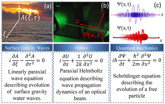
Figure 1.
(a) Ocean surface gravity water waves propagating according to the linear paraxial wave equation. (b) A green laser beam () propagating in free space, according to the paraxial Helmholtz equation. (c) An illustration of Gaussian (top) and Airy (bottom) wavefunctions which are solutions of the Schrödinger equation of a free particle.
2. Mathematical Introduction
2.1. Governing Equations
In this section, we introduce equations that govern evolution of surface gravity water waves, which are necessary to describe analogous experiments in optics and in quantum mechanics.
The extent of nonlinearity in the analysis of water gravity waves is determined by wave steepness , where k and a denote characteristic wave number and amplitude, respectively. In linear approximation, the evolution in space x of the envelope of a unidirectional narrow-banded wave train is described by the Schrödinger equation, see, e.g., [22,23].
The spatial coordinates x is pointed in the propagation direction and t is the time.
Applying scale-separation analysis, Zakharov derived a general equation, which describes the temporal evolution of nonlinear deep-water gravity waves in wave-vector Fourier space that is accurate up to the 3rd order in the wave steepness [24]. In the same paper, it was demonstrated that for vanishingly narrow spectrum, water-waves are governed by the Nonlinear Schrödinger equation (NLSE) that describes the evolution of the scaled complex wave packet envelope in the physical space:
The scaled dimensionless variables are related to the propagation coordinate x and the time t by and and is the group velocity. The carrier wave number and the angular carrier frequency satisfy the deep-water dispersion relation , with g being the gravitational acceleration, and define the group velocity .
Dysthe [25] suggested a 4th order modification of NLSE by somewhat relaxing the requirement on the spectral width. The spatial version of the Dysthe equation in normalized form is given by [26,27]
Here represents the envelope of the velocity potential. , and . The spatial coordinate z is a vertical coordinated pointed up vercially, at the free surface.
All physical diverse phenomena considered here represent propagating wavepackets. Despite that different nature, the propagation of these wavepackets can be described mathematically by the same Schrödinger equation. Note that conditions defining the domain of validity of this equation depend on the physics of the phenomena. In the next chapter, this equation is derived for wavepackets for quantum mechanics, optics and surface water gravity waves.
2.2. The Schrödinger Equation Describing the Evolution of Linear Wavepackets of Various Physical Nature
Wavepackets, or wave trains, are solutions of various wave-equations in physics that are characterized by frequency and wavenumber [4]. Wavepackets often describe short bursts of localized wave actions and usually travel as one entity in space and time. Wavepackets are defined by their phases and amplitudes so that they interfere constructively only over a small region of space (or time), and lose coherence elsewhere in space (or time) [28]. In quantum mechanics, wavefunctions are used to describe the probability distribution of quantum mechanical particles and their evolution in space and time. In optics, wavepackets usually describe the temporal variations of short light pulses and/or the spatial variation of optical beams traveling in a dielectric medium [29]. In this chapter, we derive the Schrödinger equation for the evolution in space/time for traveling wavepackets in quantum mechanics, optics and surface gravity water-waves.
2.2.1. The Schrödinger Equation in Quantum Mechanics
In quantum mechanics, we consider, for simplicity, a plane wave traveling in space and time [8]. The complex-valued wavefunction is given by
where is the angular frequency and k is the wave number related to the wavelength by . is a wavefunction. This wavefunction defines a propability amplitude of a quantum state of a certain isolated quantum system. Each measurable physical quantity of the system can be determined from [4].
Partial derivation with respect to time of gives
Substituting the Plank-Einstein relation for the matter-waves in Equation (5) leads to
For a free particle, the energy is given by where p is obtained from de-Broglie relations and given by . As a result, the energy is given by .
Taking the 2nd partial derivative of with respect to space yields
Comparison with Equation (6) results in the familiar expression for the Schrödinger equation.
2.2.2. The Schrödinger Equation in Optics
In optics, the Schrödinger equation is an approximation, via the slowly varying envelope method, of the Helmholtz equation. To derive the Helmholtz equation for electromagnetic waves in MKS units, we first consider the wave equation, which is easily obtained from Maxwell’s equations [3].
where is the electric field, is the magnetic field and and are the permittivity and permeability constants in vacuum respectively.
Taking the curl of Equations (9) (ii, iv) yields
Using the vector identities together with and Equation (9) (i, iii) results in the wave equation for electromagnetic waves.
where c is the speed of light in vacuum.
We shall now focus on the electric field. The Helmholtz equation can also be derived for the magnetic field in a similar manner. We assume that the electric field is in fact separable
Substituting Equation (12) into the wave equation for the electric field, resulting in
The left side of Equation (13) depends on x while the right side depends on t. To derive the Schrödinger equation for optics we are interested solely in the spatial domain, i.e., in the left side of Equation (13) that represents the spatial Helmholtz equation in optics
where .
Invoking the slowly varying envelope approximation (SVEA), the envelope of an electromagnetic wavepacket may been seen as slowly varying in the z direction [29]. We assume a solution to Equation (14) of the following form
where is the amplitude of the traveling wave at the origin. Thus, the second derivative of is given by
Substituting Equation (16) into the Helmholtz equation gives
Finally, under the SVEA condition, ; considering a linearly polarized electromagnetic wave in the x direction we get
which is the Schrödinger equation in the field of optics. This equation usually used to describe a linearly polarized electromagnetic wave, propagating in the z direction.
2.2.3. Linear Schrödinger Equation For Narrow-Banded Surface Gravity Waves
In hydrodynamics, the Linear Schrödinger Equation is used to model the propagation of narrow-banded surface gravity waves [22]. The surface elevation can be represented by using the complex normalized envelope , where x is a spatial coordinate and t is a temporal coordinate. For narrow-banded wavepacket with the carrier frequency and a carrier wave number
Multiplying Equation (19) by results in
Expanding the dispersion relating around yields
where is the the group velocity, and
Up to the 2nd order in , the time derivative of is thus,
Since multiplication by ik in Fourier space is equivalent to differentiation in x in the physical space, Equation (23) in the physical space is
Define , and , thus in the frame of references moving with the linear Schrödinger equation assumes the following form
Note that, the whole derivation is limited to a linear case. For steeper waves high order extensions in are available, such as NLSE and modified NLSE (see Equations (2) and (3)) or Ref. [27].
2.3. Wavepackets
In this section we will review the most commonly used wavepackets in quantum mechanics and optics and discuss their unique properties. The wavepackets considered in this article are solutions of the linear Schrödinger equation. To illustrate the shapes of the wavepackets discussed in sequel, we plot the absolute values of the envelopes and the phases are presented in Figure 2, Figure 3 and Figure 4 respectively.
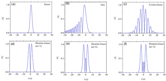
Figure 2.
Envelopes (blue curves) of different wavepackets presented in this chapter for . (a) Gaussian packet , with duration s; (b) Airy wave packet , with truncation and width of main lobe s. (c) Cosine-Gauss packet , with rad/s, , s. (d–f) Hermite-Gauss packet with different order , where is Hermite polymial and s.
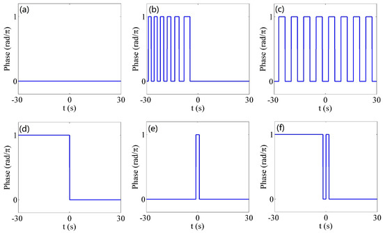
Figure 3.
Envelope Envelope phases (blue curves) of different wavepackets presented in this chapter for . (a) Gaussian packet , with duration s; (b) Airy wave packet , with truncation and width of main lobe s. (c) Cosine-Gauss packet , with rad/s, , s. (d–f) Hermite-Gauss packet with different order , where is Hermite polymial and s.
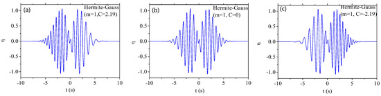
Figure 4.
Envelopes (blue curves) of the Hermite-Gauss packet with different order , where is Hermite polynomial. HG1 envelope function with carrier wave and chirp, given by , with, (a) (b) , and (c) ; s; rad/s.
2.3.1. Gaussian Wavepackets
In quantum mechanics, the simplest way to describe a large number of simultaneously excited quantum levels is to use a wave function with the Gaussian distribution. Such wave functions are often refereed to as Gaussian wavepackets and they describe a quantum mechanical point particle [30]. In optics, electromagnetic pulses with a Gaussian distribution are widely used. For instance, ultra-fast light pulses are usually generated with a Gaussian distribution in the temporal domain whereas the spatial distribution of the light emitted from most lasers is also Gaussian [29]. In surface gravity water-waves, Gaussian wavepackets can be generated by a mechanical wave maker using an appropriate driving signal [22]. The temporal variation of the surface elevation with the Gaussian envelope given by
is prescribed by the wavemaker at , with defining the initial pulse width. The absolute value of the envelope of such a wavepacket at different positions and times is given by
and its phase by
where , the normalized temporal coordinate is and is the Gouy phase. Note that the values of A are normalized by the maximum amplitude . Equations (27) and (28) are given in the moving frame while Equation (26) is given in the laboratory frame.
2.3.2. Hermite-Gauss Wavepackets
Hermite-Gauss wavepackets are higher-order solutions of the paraxial Helmholtz equation in Cartesian coordinates. These wavepackets are widely used to optics, as they possess several characteristic features [31]. As such, Hermite-Gauss beams evolve self-similarly in space, maintaining their initial profiles. In addition, for the same Gaussian width, the higher-order beam width (defined by the square root of the second-order moment) is m times larger than the width of the respective fundamental beam, where m is related to the order of Hermite function. Finally, since they form a complete orthogonal set, any scalar wave in Cartesian coordinates can be decomposed into a combination of Hermite-Gauss components. These properties make the Hermite-Gauss very useful for studying processes of optical vortex generation, mode conversion, beam shaping and second harmonic generation. The Hermite-Gauss envelope of the temporal surface elevation is given by
where represents the Hermite polynomial of order m, is the characteristic envelope duration, and the chirp coefficient C is used to control the quadratic modulation of the phase of the incident pulses, so that the envelope A becomes linearly frequency chirped. Integrating the Schrödinger equation with this initial condition yields
where
is the variation of envelope amplitude and phase, respectively. In this case and the constant , depends linearly on the chirp coefficient. represents the propagated Hermite polynomial.
2.3.3. Cosine-Gauss Wavepackets
In optics, non-diffracting beams are widely used for various applications [32]. These unique waves keep their original shape in space and time, as opposed to beams of light which diffract while propagating over a certain distance or time. The cosine-Gauss optical beam is an example of a non-diffracting wave packet [33,34]. Due to analogies between optics and hydrodynamics, a linear surface gravity water wave with cosine-Gauss envelope also can resist the inherent dispersion during propagation. It should be noted that while in optics this wavepacket is non-diffracting, in hydrodynamics it is effectively non-dispersive. The cosine-Gauss temporal variation of the water surface elevation at the wavemaker is given by
where can be seen as a half-intersecting angle of two plane waves truncated by a Gaussian envelope of finite duration . Integrating this initial condition using the Schrödinger equation yields
where
and are envelope and phase, respectively, and .
One can notice that Equation (36) shows that the two wavepackets become gradually separated in time in course of their propagation. However, for the right choice of parameters and , the quantity becomes constant and . As a result, these truncated waves approximately overlap during propagation over a limited distance, which gives rise to a non-spreading behaviour of cosine-Gauss wavepackets.
2.3.4. Airy Wavepackets
The Airy wavepacket accelerates without any external force and preserves its shape in a dispersive medium. Berry and Balzas showed that the Airy wavepacket is a solution of the Schrödinger equation for a free particle [35]. Since then, the Airy wavepackets were extensively studied in various subfields in optics and quantum mechanics. In 2007 Christodoulides and coworkers showed that an ideal Airy optical beam follows a bent parabolic trajectory in free space and remains diffraction-free [36]. Furthermore, Airy beams were used for optical manipulation of micro-particles, generation of curved plasma channels, light induced optical routing, and superresolution fluorescence imaging [37,38,39,40]. Airy wavepackets were also studied in the nonlinear regime, including the nonlinear optical generation and the evolution of Airy beams in various quadratic, cubic, and photorefractive media [41,42,43]. In contrast to other wave packets considered here, an ideal Airy water-wave train carries an infinite amount of energy, whereas in practice these pulses are truncated by an exponential or a Gaussian window. Here we use an exponential truncation; thus, the Airy envelope of the temporal surface elevation is given by
where and denote the characteristic duration and the positive truncation parameter, gives rise to the Airy pulse with the amplitude
and the phase given by
where .
2.3.5. The Temporal Slit
When light passes through a slit with width d of the order of the wavelength of the light, a single slit diffraction pattern can be observed on a screen at a distance from the slit. According to intuition we gain from classical physics, a wave that has passed through a slit will expand. However, this picture is incomplete; it was predicted [44] that a rectangular one-dimensional quantum wave packet created from a plane wave by a one-dimensional slit first focuses and only then expands. This phenomenon can be described by applying the Schrödinger equation. Consider a rectangular one dimensional wave packet of constant phase during the early stage; in the paraxial wave approximation it is identical to the diffraction of a scalar field from a single slit. In such a case, the wave packet can exhibit self-focusing. To model this phenomenon in surface gravity water waves, temporal and spatial coordinates have to be interchanged. Hence, to observe this focusing in experiments on water waves, one must consider a temporal slit, as has been recently done [45].
The temporal rectangular water wave packet of width generated at at the wave maker has the envelope
Its evolution along the water tank is described by
where is a dimensionless constant which is proportional to the width of the initial rectangular envelope Hence, the temporal variation of the surface elevation for a carrier wave with the frequency and wave number is .
3. Experiments on Water-Wave Packets
3.1. Experimental Facility and Procedure
The experiments discussed in this paper were performed in a long, wide, and deep laboratory wave tank, see Figure 5. Water waves are generated by a computer-controlled wavemaker, that consists of four synchronously-moving paddle-type modules and placed at one end of the tank. The carrier wave numbers in all experiments satisfy the deep-water condition [10], and the wave dissipation can be neglected.
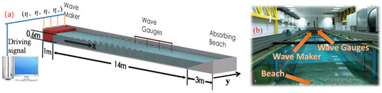
Figure 5.
(a) Schematic illustration of the experimental setup for generating surface gravity water wave packets (b) Photograph of the experimental facility.
Wave energy absorbing beach placed at the far end of the tank is also shown in Figure 5. To mitigate effect of residual reflections from the beach, measurements are performed at distances between to . The instantaneous water surface elevation at any fixed location along the tank is measured by four wave gauges mounted on a bar parallel to the tank side walls. The bar with the gauges is fixed to an instrument carriage that can move along the tank, its displacement is controlled by the computer. The control of the wavemaker by computer enables synchronization of its operation with the wave gauge data acquisition using LabView software.
3.2. Linear Dynamics
In this section we review some of the recent experimental results on surface gravity water waves in the linear regime that can be adequately described by the Schrödinger equation.
These importance of those results is in the similarity of their physics to non-relativistic quantum theory.
For example, the important properties of the Airy wave packet such as shape preservation in dispersive medium and acceleration without application of external force were recently observed by Shenhe Fu et al. [9] in surface gravity water waves, as seen in Figure 6a–c. The mean value of the main lobe of Airy and inverted Airy wave packets were plotted and compared with Gaussian wave packets, Figure 6d. In their experiments, Shenhe Fu et al. saw for the first time that Airy wave packets self-decelerate, while inverted Airy wave packets self-accelerate. This behavior is opposite to the expected for a free particle in quantum mechanics. The difference stems from the fact that in the version of the Schrödinger equation describing surface gravity water waves, the spatial and temporal coordinates are interchanged as compared to the Schrödinger equation in quantum mechanics (see Equation (2)). Shenhe Fu et al. succeeded in demonstrating in their water waves experiments the diverse features of the propagation dynamics of Airy water wave pulses, such as nonspreading, self accelerating, and self-healing properties, as seen in Figure 6f–g.
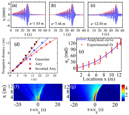
Figure 6.
Experimental elevations (blue curves) and theoretical envelopes (red curves) of Airy wave packets measured at (a) x = 1.43 m, (b) 7.46 m, and (c) 12.50 m, for = 6 mm ( = 0.05), = 0.1, and = 2.0 s, (d) the parabolic trajectories of Airy and inverted Airy wave packets, using = 0.7 s and = 5 mm, (e) The phase offset as a cubic function of x. Evolution of Airy envelopes obtained from the measurements by the Hilbert transform of the recorded surface elevation variation with time; (g) Airy envelopes simulated using Equation (1) with = 0.65 s and = 0.1, in a frame of reference moving at .
An additional important feature of Airy wave packets is the accumulation of phase proportional to . This cubic-phase offset was predicted more than 40 years ago [35,46] and was measured in water waves for the first time [18], see Figure 6e. It should be stressed that in quantum mechanics and in optics, the measurement of the phase of a wave packet is practically impossible, since only the signal intensity of the high carrier frequency can be measured and therefore the information on the phase is lost [47]. Hence, the possibility to measure wave packets governed by the Schrödinger equation in surface gravity water waves not only provides verification of experimental results obtained in totally different physical systems, but also serves as a valuable tool to observe fundamental properties of wave packets which are inaccessible in other fields.
Recently, new shapes of linearly non-dispersive surface gravity water wave packets have been observed. These include wavepackets with a cosine-Gauss envelope, as shown in Figure 7 and Figure 8, as well as its higher-order Hermite cosine-Gauss variations [48,49]. It was shown that these wave envelopes preserve their width despite the inherent dispersion of water gravity waves. Furthermore, it was observed that these wave packets exhibit self-healing; i.e., they are restored after passing an obstacle, as shown in Figure 7.
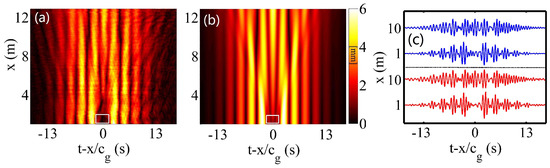
Figure 7.
A theoretical plot and experimental verification of the self-healing property of surface gravity wavepackets with a Cosine-Gauss shape. The related parameters are: , , s. (a) Experiment and (b) simulation for the pulse envelope evolutions. (c) The measured elevation wave groups at two different locations. The blue curves are given by a simulation while the red curves are given by an experiment.
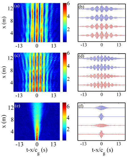
Figure 8.
Propagation dynamics of cosine-Gauss pulses along the tank presented in Figure 7 with = 6 mm ( = 0.05), , and = 9.0 s (a,b) and for (c,d). (a,c) Experimental results on pulse envelopes obtained by the Hilbert transform in a frame of reference moving at velocity ; (b,d) temporal variation of the surface elevation at two locations; (e,f) Gaussian pulse evolution, the initial width of the Gaussian pulse as in (a).
The propagation dynamics of surface gravity water-wave pulses having Hermite-Gauss (HG) envelopes was studied in [11]. These wave packets also propagate self-similarly along an a wave tank, preserving their envelopes, see Figure 9 [50]. The measured surface elevation of the wave groups enabled observing the envelope phase evolution of both non-chirped and linearly frequency chirped pulses, hence making possible measurement of the Gouy phase shifts of high-order HG wave packets, see Figure 10 [51].
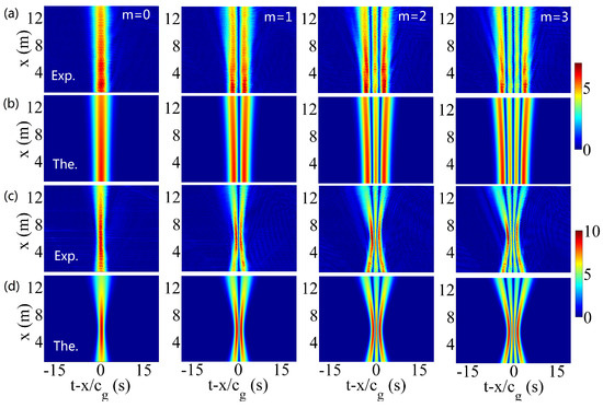
Figure 9.
The evolution of envelopes of the non-chirped and linearly chirped Hermite-Gauss (HG) wave pulses, with = 6 mm, = 2.5 s, and C = 0 (a,b), C = −2.19 (c,d) for different m (see the top). In the experiments, the pulse envelopes were obtained using Hilbert transform of the measured elevations, in a frame of reference moving at . The color bar units of the envelope are mm. (a,c) The measurements; (b,d) the theoretical results based on Equation (30).
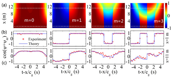
Figure 10.
The carrier-envelope phase of the non-chirped HG pulses demodulated from the measured water surface elevation variation with time, with = 6 mm, = 2.5 s, and C = 0. The envelope phase is presented as a cosine function of time. (a) Two-dimensional phase map calculated from Equation (32) for different order of m. (b,c) The envelope phase profiles at x = 1 m (b) and x = 11 m (c). The blue curves in (b,c) correspond to the theory, while the red scattered dots denote the experiments.
As already stressed, the phase of a wave function is usually inaccessible in optical experiments, owing to the high carrier frequency ( Hz). The carrier frequencies of water waves are lower by many orders of magnitude. It is therefore relatively easy to demodulate the envelope phase of these HG pulses. In [9], the envelope phase of these pulses was determined directly by extracting the local maximum and minimum values of the elevations. Figure 5a illustrates the theoretically calculated envelope phase variation with t and x for different orders m of HG waves. For better visibility, temporal envelope phase variation at two locations, x = 1 m and x = 11 m, is plotted, see Figure 5b,c. To avoid phase ambiguity, the results are presented in a form of cosine function, i.e., .
3.3. Nonlinear Dynamics
Quantum theory deals only with the linear Schrödinger equation. However, in optics, electromagnetic waves interact with matter in such a way that they can be described by the Nonlinear Schrödinger equation (NLSE). The nonlinearity of wave propagation leads to such effects as second harmonic generation, cubic Kerr nonlinearity, self-focusing (or defocusing) and more [52,53]. In surface gravity water waves, nonlinear effects become prominent when the wave steepness is high, typically > 0.1, and have been extensively studied for decades. Nonlinear effects for Airy wave packets indeed are observable when the carrier wave steepness is increased, and manifest themselves e.g., by the generation of water-wave solitons as seen in Figure 11.
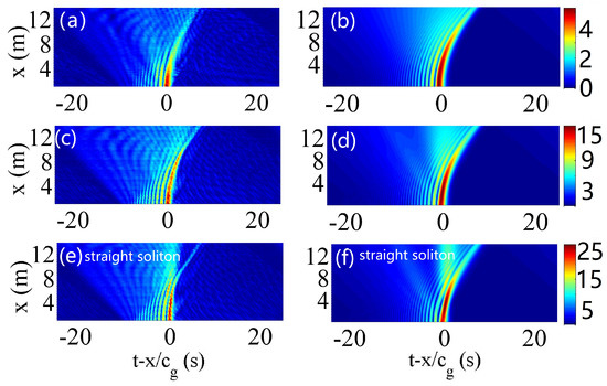
Figure 11.
Evolution of Airy envelopes obtained from the experimental records by the Hilbert transform (a,c,e) and simulated using Equation (1) (b,d,f) with = 0.65 s and = 0.1, in a frame of reference moving at velocity Measurements were performed at (a,b) = 5 mm, = 0.04, (c,d) = 17 mm, = 0.14, and (e,f) = 23 mm, = 0.19.
When the maximum amplitude in the wave packet was increased to = 17 mm, it was observed that the Airy pulses stabilized. In this case, not only did they self-accelerate along the parabolic trajectory, but the dispersion was compensated by nonlinearity. For an even higher amplitude = 23 mm, strong Kerr-type nonlinearity appears. In this case, the central lobe of the Airy pulse compresses during propagation, further increasing its amplitude, which eventually leads to a collapse and an emission of a stationary soliton, shown in Figure 11e,f. Apart of Airy pulses, cosine-Gauss pulses, as well as its higher-order Hermite cosine-Gauss variations, were also extensively studied in nonlinear optics [54] and recently in surface gravity water waves [9]. The earlier research on cosine-Gauss waves was limited to the linear approximation [33,49,55]; the propagation dynamics of those wave packets in a nonlinear dispersive medium was never explored. Investigation of Hermite-cosine-Gauss (HCG) pulses by Shenhe Fu et al. [10] is based on the modified NLS Equation (1). Whereas the HCG0 (order m = 0) wave maintains maximum intensity at the center of the pulse, the HCG1 (m = 1) pulse has zero intensity at the center, but preserves the two strong nearby peaks at the leading and trailing edges of the pulse; see Figure 12. For a weakly nonlinear amplitude of = 16 mm = 0.13, see Figure 9, it was found that the invariant propagation of such HCG pulses was still observed despite nonlinearity. It should be stressed that high steepness, symmetry breaking and the spectral widening observed in experiments with HCG wave envelope violate the assumptions adopted in the derivation of NLSE as discussed in [56]. The modeling was therefore based on the modified (Dysthe) nonlinear Schrödinger equation that is capable of describing the emerging envelope asymmetry and spectral widening [27].
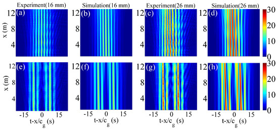
Figure 12.
Nonlinear propagation dynamics of HCG0 (a)–(d) and HCG1 (e)–(h) pulses along the tank for two amplitudes (see the top); (a)–(d) = 9 s, = 7.5° and (e)–(h) = 9 s, = 5.5°. The color bar units are millimeters.
Effects of nonlinearity have been further studied in experiments on Hermite-Gauss water wave pulses with an essentially nonlinear wave steepness [11]. Figure 13 that presents the measured envelope evolution of nonlinear non-chirped HG pulses. For higher wave steepness , the HG wave pulses contain waves at the carrier wave frequency , as well as the second-order bound waves at the frequency . The surface elevation variation with time can thus be presented as , where A and are the complex envelopes of the free and 2nd order bound waves, respectively [27]. The Figure 13 clearly shows that these nonlinear waves still maintain their self-similar propagation despite the strong nonlinearity, approximately preserving their Hermite-Gauss shapes [57,58]. Very weak free slowly propagating waves at the 2nd harmonic , generated due to the presence of the bound waves at this frequency by the wavemaker, can also be identified in Figure 13. Figure 12 and Figure 13 also indicate that for stronger nonlinearity, the HG0 pulse was seriously compressed as compared to the apparently due to nonlinearity. The compression of higher-order pulses is less pronounced; this may be associated with the smaller width of their lobes and thus wider spectra. The presented results indicate that higher-order Hermite-Gauss pulses are more resilient to nonlinear perturbations. Owing to the nonlinear effects and the resulting spectral evolution documented in Figure 14, the wave packets propagate at the velocity slightly higher than ; see Figure 13a.
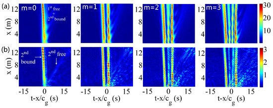
Figure 13.
Experimental results for: (a) nonlinear propagation of HG pulses and (b) the generated second harmonic bound waves with = 21 mm ( = 0.17), = 2.5 s, and C = 0. Both (a) and (b) represent the envelope in a moving system. The color bar units are millimeters.
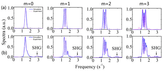
Figure 14.
The spectra of the nonchirped HG wave pulses calculated at x = 7.39 m, with = 2.5 s and C = 0. (a) The measured linear spectra with = 6 mm ( = 0.05); (b) the measured nonlinear spectra with = 21 mm ( = 0.17). Blue curves correspond to simulations based on Equation (1); the red curves denote the experiments.
To study the nonlinear effects further, the emergence of second harmonic generation is demonstrated. Spectra of nonlinear HG pulses are presented in Figure 14b [11]. The corresponding spectra of linear pulses are also shown for comparison; see Figure 14a. The spectra in both cases were obtained at a fixed location of x = 7.39 m.
In the linear case (see Figure 14a), these spectra are symmetric, for all orders , also having Hermite-Gauss shapes.
The center of the fundamental harmonic is located at . In the nonlinear regime (see Figure 14b), these spectra exhibit asymmetry and become wider, with an apparent 2nd harmonic bound waves, see also Refs. [59,60]. Despite nonlinearity, their general HG shapes remain recognizable within the dominant frequency range. This can explain the approximate conservation of the HG shapes in the course of propagation in nonlinear regime.
3.4. Diffractive Focusing
So far we have demonstrated propagating wave packets and their linear and nonlinear dynamics in surface gravity water waves. However, it was recently shown that surface gravity water waves can also be utilized to emulate geometric optical apparatus such as a single slit [29,45]. Here we present a recent results on diffractive focusing of surface gravity water wave are shown in Figure 15.
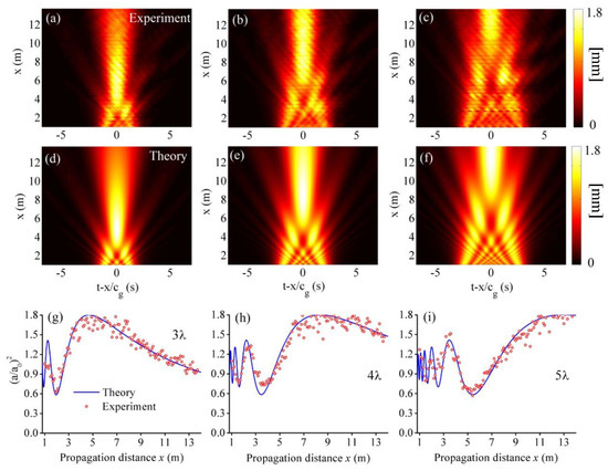
Figure 15.
Observation of diffractive focusing phenomenon of rectangular surface water-wave packet with different width: (a,d,g) s; (b,e,h) s; and (c,f,i) s. The incident amplitude is . (a–c) Experimental results representing the normalized intensity evolution () of the wave packets along the tank; while (d–f) illustrate the corresponding theoretical results. (g–i) depict the on-axis () intensity variation of the wave packets.
Figure 15 demonstrates both experimentally and theoretically the diffractive focusing feature of the generated rectangular surface water-wave packets. In the experiments, we set = 6 mm () so that the induced nonlinearity could be neglected. At the beginning, the propagation dynamics of such wave packets with s, s and s were investigated, see Figure 15a,d,g, Figure 15b,c,h and Figure 15c,f,i respectively. In order to illustrate the focusing effect, the recorded elevations were represented in a system traveling at the linear group velocity . The pulse envelope can be obtained by Hilbert transforming the elevations. As expected, these wave packets indeed exhibit diffractive focusing property, as evident from their intensity evolution along the tank, see Figure 15a–c for three cases of wave packets. Clearly, all the results show significant shrinking at their early stage of propagation. The experimental results match well with the theory. We further observed the on-axis intensity variation along the tank, see Figure 15g–i. Their intensity first oscillates with the distance; then increasing the propagation distance, the intensity reaches its maximum value, nearly times larger than the initial value, which further confirms the diffractive focusing phenomenon of the wave packets. It is worth noting that the calculated and observed intensity patterns from Figure 15 are similar to those observed by Vitrant et al. [61]. for the case of light beams diffracting from a slit. We emphesize that one can now place another slit at the focal point and further focus the pulse, since the phase distribution in the focal region is similar to that at the origin. This property was demonstrated in the spatial domain using surface plasmon polariton waves [45].
4. Conclusions
In summary, numerous examples presented here demonstrate essential features that are common to propagation of hydrodynamics surface water gravity wave trains and quantum mechanical wavefunctions and electromagnetic pulses and optical beams. All these wave phenomena can be described at the linear level by the Schrödinger equation and by its extension to the nonlinear Schrödinger equation (NLSE) when nonlinear effects become prominent. For the hydrodynamic waves, these equations describe fairly accurately the evolution in space and time of the complex envelope of a narrow-banded wave train. It should be stressed that linear and nonlinear surface water-waves have been studied extensively since the groundbreaking work by Stokes in mid-ninetieth century. These studies included developments of more advanced theoretical models that overcame the limitations of the NLSE. Quantitative and qualitative experimental verification of the theoretical model equations has been carried out that established limits on the validity of their application for diverse conditions. The similarity of the governing equations suggests that some of the well known results accumulated in hydrodynamic studies may be readily applicable to other branches of physics dealing with wave propagation.
Naturally, an emphasis on certain shapes of wave packets and of quantum mechanical wave functions can be of lesser interest for purely hydrodynamic studies. However, surface gravity wavepackets of various shapes are observable by a naked eye and can be easily generated in laboratory facilities. These hydrodynamic waves are easily accessible, they propagate relatively slowly and are characterised by time and length scale much longer that those of light beams. These features enable accurate measurements in water-wave tanks of numerous wave packet parameters relevant to optical beam propagation with details that cannot be reproduced in experimental studies in optics and quantum mechanics.
We have reviewed here numerous examples of surface gravity water wave trains and their analogies to quantum mechanical wave-functions or optical beams. Specifically, we discuss the first observation for the propagation dynamics in both the linear and the nonlinear regimes of Airy wave packets (that actually emerged initially in studies of water waves), as well as of cosine-Gauss and Hermite-Gauss water-wave pulses. In the linear regime, we consider the nonspreading, self-accelerating, and self healing properties of these pulses. Furthermore, we have reviewed the case of a diffraction from a slit and discussed how water waves experience the effect of diffractive focusing by a temporal or a spatial slit.
The slow scales of surface gravity waves make possible verification in the experiments of phase evolution patterns in optical beams that have been predicted many years ago. Furthermore, we have discussed cases of nonlinear propagation. It should be stressed that the NLSE retains the initial symmetry of the pulse. Nonlinearity often gives rise to wave envelope asymmetry and to spectral broadening; to account for these phenomena the Dysthe equation (MNLSE) has been applied as the theoretical model.
We believe these analogies benefit quantum mechanics and optics, as they allow to reproduce diverse phenomena in the hydrodynamical setting that make possible detailed measurements of the spatial and temporal wavepackets evolution. The advantage of measuring surface gravity water-waves in hydrodynamics is the ability to record the full waveform of the wave, owing to its low carrier frequency. In contrary to that, optical and matter waves are typically characterized by very high carrier waves, usually much higher than that of the system used to measure them, hence in these disciplines it is more common to measure the the squared amplitude of the wavepacket (i.e., its intensity), thus the phase information of the wave is lost. In contrary to that, the advantage of optical waves with respect to surface gravity water wavepackets is that it is fairly easily to repeat many times an optical experiment in a short time, which is important for obtaining the statistics of a process.
In addition, observation of wavepacket dynamics in a mechanical system may provide a new insight to the behavior of the corresponding wave forms in different physical conditions. We are convinced that the field of hydrodynamics can also highly benefit from this type of research, as it gains from the mathematical and physical concepts imported from quantum mechanics and optics. As such, self-acceleration of wavepackets, self-healing and non-spreading properties.
Author Contributions
The paper concept was proposed and edited by G.G.R., and all authors contributed to the preparation of it.
Funding
This work was supported by DIP, the German-Israeli Project cooperation, Israel Science Foundation, grant 306/15 and Natural Science Foundation of Guangdong Province, grant 2017B030306009.
Acknowledgments
We acknowledge Wolfgang P. Schleich, Maxim Efremov, Matthias Zimmermann, Alona Maslennikov and Anatoliy Khait for fruitful discussions on related topics.
Conflicts of Interest
The authors declare no conflict of interest.
References
- Pain, H.J. The Physics of Vibrations and Waves, 6th ed.; Wiley: Hoboken, NJ, USA, 2006; ISBN 0471985422. [Google Scholar]
- Faber, T. Fluid Dynamics for Physicists; Cambridge University Press: Cambridge, UK, 1995; ISBN 9780511806735. [Google Scholar]
- Jackson, J.D. Classical Electrodynamics, 3rd ed.; Wiley: Hoboken, NJ, USA, 1998; ISBN 9780471309321. [Google Scholar]
- Griffiths, D.J. Introduction to Quantum Mechanics; Wiley: Hoboken, NJ, USA, 1998; ISBN 9780471309321. [Google Scholar]
- Danon, J.; Nazarov, Y. Advanced Quantum Mechanics: A Practical Guide; Cambridge University Press: Cambridge, UK, 2013; ISBN 9780521761505. [Google Scholar]
- Feynman, R.P.; Leighton, R.B.; Sands, M. The Feynman Lectures on Physics, Vol. I: The New Millennium Edition: Mainly Mechanics, Radiation, and Heat; Wiley: Hoboken, NJ, USA, 1998; ISBN 9780471309321. [Google Scholar]
- Feynman, R.P.; Leighton, R.B.; Sands, M. The Feynman Lectures on Physics, Vol. II: The New Millennium Edition: Mainly Electromagnetism and Matter (Feynman Lectures on Physics); Wiley: Hoboken, NJ, USA, 1998; ISBN 0465024165. [Google Scholar]
- Feynman, R.P.; Leighton, R.B.; Sands, M. The Feynman Lectures on Physics, Vol. III: The New Millennium Edition: Quantum Mechanics (Feynman Lectures on Physics); Wiley: Hoboken, NJ, USA, 1998; ISBN 9780465025015. [Google Scholar]
- Fu, S.; Tsur, Y.; Zhou, J.; Shemer, L.; Arie, A. Propagation Dynamics of Airy Water-Wave Pulses. Phys. Rev. Lett. 2015, 115, 034501. [Google Scholar] [CrossRef]
- Fu, S.; Tsur, Y.; Zhou, J.; Shemer, L.; Arie, A. Propagation Dynamics of Nonspreading Cosine-Gauss Water-Wave Pulses. Phys. Rev. Lett. 2015, 115, 254501. [Google Scholar] [CrossRef]
- Fu, S.; Tsur, Y.; Zhou, J.; Shemer, L.; Arie, A. Self-similar propagation of Hermite-Gauss water-wave pulses. Phys. Rev. E 2016, 93, 013127. [Google Scholar] [CrossRef]
- Berry, M.V.; Chambers, R.G.; Large, M.D.; Upstill, C.; Walmsley, J.C. Wavefront Dislocations in the Aharonov-Bohm Effect and its Water Wave Analogue. Eur. J. Phys. 1980, 1, 154. [Google Scholar] [CrossRef]
- Bar-Ziv, U.; Postan, A.; Segev, M. Observation of Shape-preserving Accelerating Underwater Acoustic Beams. Phys. Rev. B. 2015, 92, 100301. [Google Scholar] [CrossRef]
- Chabchoub, A.; Kibler, B.; Finot, C.; Millot, G.; Onorato, M.; Dudley, J.M.; Babanin, A.V. The Nonlinear Schrödinger Equation and the Propagation of Weakly Nonlinear Waves in Optical Fibers and on the Water Surface. Ann. Phys. 2015, 361, 490–500. [Google Scholar] [CrossRef]
- Chabchoub, A.; Hoffmann, N.P.; Akhmediev, N. Rogue Wave Observation in a Water Wave Tank. Phys. Rev. Lett. 2011, 106, 204502. [Google Scholar] [CrossRef] [PubMed]
- Dudley, J.M.; Erkintalo, M.; Genty, G. Rogue-wave-like Characteristics in Femtosecond Supercontinuum Qeneration. Opt. Photonics News 2015, 26, 34–41. [Google Scholar] [CrossRef]
- Dudley, J.M.; Dias, F.; Erkintalo, M.; Genty, G. Instabilities, Breathers and Rogue Waves in Optics. Nat. Photonics 2014, 8, 755. [Google Scholar] [CrossRef]
- Rozenman, G.G.; Zimmermann, M.; Efremov, M.A.; Schleich, W.P.; Shemer, L.; Arie, A. Amplitude and Phase of Wavepackets in Linear Potential. Phys. Rev. Lett. 2019, 122, 124302. [Google Scholar] [CrossRef]
- Bush, J.W.; Couder, Y.; Gilet, T.; Milewski, P.A.; Nachbin, A. Chaos: An Interdisciplinary. J. Nonlinear Sci. 2018, 28, 096001. [Google Scholar]
- Bush, J.W. Pilot-Wave Hydrodynamics. Annu. Rev. Fluid Mech. 2015, 47, 269–292. [Google Scholar] [CrossRef]
- Milewski, A.P.; Wang, Z. Self-focusing Dynamics of Patches of Ripples. Phys. Nonlinear Phenom. 2016, 333, 235–242. [Google Scholar] [CrossRef]
- Mei, C.C. Theory and Applications of Ocean Surface Waves; World Scientific: Singapore, 2005; ISBN 9789812388933. [Google Scholar]
- Sutherland, B.R. Internal Gravity Waves; Wiley: Hoboken, NJ, USA, 2010; ISBN 9780521839150. [Google Scholar]
- Zakharov, V.E. Stability of Periodic Waves of Finite Amplitude on the Surface of a Deep Fluid. J. Appl. Mech. Tech. Phys. 1968, 9, 190–194. [Google Scholar] [CrossRef]
- Dysthe, K.B. Note on a Modification to the Nonlinear Schrödinger Equation for Application to Deep Water Waves. Proc. R. Soc. A 1979, 369, 105–114. [Google Scholar] [CrossRef]
- Lo, E.; Mei, C.C. A Numerical Study of Water-wave Modulation Based on a Higher-order Nonlinear Schrödinger Equation. J. Fluid Mech. 1985, 150, 395–416. [Google Scholar] [CrossRef]
- Shemer, L.; Dorfman, B. Experimental and Numerical Study of Spatial and Temporal Evolution of Nonlinear Wave Groups. Nonlin. Process. Geophys. 2008, 15, 931–942. [Google Scholar] [CrossRef]
- Blokhintsev, D.I. Foundations of Quantum Mechanics; Springer: Berlin, Germany, 1964; ISBN 978-94-010-9711-6. [Google Scholar]
- Saleh, B.E.A.; Teich, M.C. Fundementals of Photonics; Wiley: Hoboken, NJ, USA, 1993; ISBN 9780471839651. [Google Scholar]
- Feynman, R.P.; Hibbs, A.R. Quantum Mechanics and Path Integrals; McGraw-Hill: New York, NY, USA, 1965. [Google Scholar]
- Da Silva, H.J.A.; O’Reilly, J.J. Optical Pulse Modeling with Hermite-Gaussian Functions. Opt. Lett. 1989, 14, 526–528. [Google Scholar] [CrossRef]
- Bouchal, Z. Nondiffracting Optical Beams: Physical Properties, Experiments, and Applications. Czeck Phys. 2003, 53, 537–578. [Google Scholar] [CrossRef]
- Lin, J.; Dellinger, J.; Genevet, P.; Cluzel, B.; de Fornel, F.; Capasso, F. Cosine-Gauss Plasmon beam: A Localized Long-range Nondiffracting Surface wave. Phys. Rev. Lett. 2012, 109, 093904. [Google Scholar] [CrossRef]
- Li, L.; Li, T.; Wang, S.M.; Zhu, S.N. Plasmonic Airy Beam Generated by In-Plane Diffraction. Phys. Rev. Lett. 2013, 110, 046807. [Google Scholar] [CrossRef]
- Berry, M.V.; Balazs, N.L. Nonspreading Wave Packets. Am. J. Phys. 1979, 47, 264–267. [Google Scholar] [CrossRef]
- Siviloglou, G.A.; Broky, J.; Dogariu, A.; Christodoulides, D.N. Observation of Accelerating Airy Beams. Phys. Rev. Lett. 2007, 99, 213901. [Google Scholar] [CrossRef]
- Baumgartl, J.; Mazilu, M.; Dholakia, K. Optically Mediated Particle Clearing Using Airy wavepackets. Nat. Photonics 2008, 2, 675. [Google Scholar] [CrossRef]
- Polynkin, P.; Kolesik, M.; Moloney, J.V.; Siviloglou, G.A.; Christodoulides, D.N. Curved Plasma Channel Generation Using Ultraintense Airy beams. Christodoulides. Science 2009, 324, 229–232. [Google Scholar] [CrossRef]
- Rose, P.; Diebel, F.; Boguslawski, M.; Denz, C. Broadband Acoustic Focusing by Airy-like Beams Based on Acoustic Metasurfaces. Appl. Phys. Lett. 2013, 102, 101101. [Google Scholar] [CrossRef]
- Jia, S.; Vaughan, J.C.; Zhuang, X. Isotropic 3D Super-resolution Imaging With a Self-bending Point Spread Function. Nat. Photonics 2014, 8, 302. [Google Scholar] [CrossRef] [PubMed]
- Ellenbogen, T.; Bloch, N.V.; Padowicz, A.G.; Arie, A. Nonlinear Generation and Manipulation of Airy Beams. Nat. Photonics 2009, 3, 395. [Google Scholar] [CrossRef]
- Dolev, I.; Kaminer, I.; Shapira, A.; Segev, M.; Arie, A. Experimental Observation of Self-Accelerating Beams in Quadratic Nonlinear Media. Phys. Rev. Lett. 2012, 108, 113903. [Google Scholar] [CrossRef]
- Kaminer, I.; Segev, M.; Christodoulides, D.N. Self-Accelerating Self-Trapped Optical Beams. Phys. Rev. Lett. 2011, 106, 213903. [Google Scholar] [CrossRef]
- Gonçalves, M.R.; Case, W.B.; Arie, A.; Schleich, W.P. Single-slit Focusing and Its Representations. Appl. Phys. B 2017, 123, 121. [Google Scholar] [CrossRef]
- Weisman, D.; Fu, S.; Goncalves, M.; Shemer, L.; Zhou, J.; Schleich, W.P.; Arie, A. Diffractive Focusing of Waves in Time and in Space. Phys. Rev. Lett. 2017, 118, 154301. [Google Scholar] [CrossRef]
- Kennard, E.H. Zur Quantenmechanik einfacher Bewegungstypen. Zeitschrift für Physik 1927, 44, 326–352. [Google Scholar] [CrossRef]
- Zimmermann, M.; Efremov, M.A.; Roura, A.; Schleich, W.P.; DeSavage, S.A.; Davis, J.P.; Srinivasan, A.; Narducci, F.A.; Werner, S.A.; Rasel, E.M. T3-interferometer for Atoms. Appl. Phys. B 2017, 123, 102. [Google Scholar] [CrossRef]
- Vega, J.C.G.; Bandres, M.A. Helmholtz–Gauss Waves. J. Opt. Soc. Am. A 2005, 22, 289–298. [Google Scholar] [CrossRef]
- Epstein, I.; Lilach, Y.; Arie, A. Shaping Plasmonic Light Beams with Near-field Plasmonic Holograms. J. Opt. Soc. Am. B 2014, 31, 1642–1647. [Google Scholar] [CrossRef]
- Saghafi, S.; Sheppard, C.J.R.; Piper, J.A. Characterising Elegant and Standard Hermite–Gaussian Beam Modes. Opt. Commun. 2001, 191, 173–179. [Google Scholar] [CrossRef]
- Gouy, L.G. Sur la propagation anomale des ondes. Ann. Chim. Phys. Ser. 1891, 24, 145. [Google Scholar]
- Boyd, R. Nonlinear Optics, 3rd ed.; Academic Press: Cambridge, MA, USA, 2008; ISBN 9780123694706. [Google Scholar]
- Fu, S.; Zhou, J.; Li, Y.; Shemer, L.; Arie, A. Dispersion Management of Propagating Waveguide Modes on the Water Surface. Phys. Rev. Lett. 2017, 118, 144501. [Google Scholar] [CrossRef]
- Porat, G.; Dolev, I.; Barlev, O.; Arie, A. Airy Beam Laser. Opt. Lett. 2011, 36, 4119–4121. [Google Scholar] [CrossRef]
- Epstein, I.; Remez, R.; Tsur, Y.; Arie, A. Generation of intensity-controlled Two-dimensional Shape-preserving Beams in Plasmonic Lossy Media. Optica 2016, 3, 15–19. [Google Scholar] [CrossRef]
- Shemer, L. Advantages and Limitations Of the Nonlinear Schrodinger Equation in Describing the Evolution of Nonlinear Water-wave Groups. Proc. Estonian Acad. Sci. 2015, 64, 356. [Google Scholar] [CrossRef]
- Fermann, M.E.; Kruglov, V.I.; Thomsen, B.C.; Dudley, J.M.; Harvey, J.D. Self-Similar Propagation and Amplification of Parabolic Pulses in Optical Fibers. Phys. Rev. Lett. 2000, 84, 6010. [Google Scholar] [CrossRef] [PubMed]
- Anderson, D.; Desaix, M.; Karlsson, M.; Lisak, M.; Quiroga-Teixeiro, M.L. Wave-breaking-free Pulses in Nonlinear-optical Fibers. J. Opt. Soc. Am. B 1993, 10, 1185–1190. [Google Scholar] [CrossRef]
- Shemer, L.; Goulitski, K.; Kit, E. Evolution of Wide-spectrum Unidirectional Wave Groups in a Tank: An Experimental and Numerical Study. Eur. J. Mech. B Fluids 2007, 26, 193–219. [Google Scholar] [CrossRef]
- Shemer, L.; Jiao, H.; Kit, E.; Agnon, Y. Evolution of a Nonlinear Wave Field Along a tank: Experiments and Numerical Simulations Based on the Spatial Zakharov Equation. J. Fluid Mech. 2001, 427, 107–129. [Google Scholar] [CrossRef]
- Vitrant, G.; Zaiba, S.; Vineeth, B.Y.; Kouriba, T.; Ziane, O.; Stéphan, O.; Bosson, J.; Baldeck, P.L. Obstructive Micro Diffracting Structures as an Alternative to Plasmonics Nano slits for Making Efficient Microlenses. Opt. Express 2012, 20, 26542. [Google Scholar] [CrossRef]


© 2019 by the authors. Licensee MDPI, Basel, Switzerland. This article is an open access article distributed under the terms and conditions of the Creative Commons Attribution (CC BY) license (http://creativecommons.org/licenses/by/4.0/).